Efficiently Determine the Starting Sample Size for Progressive Sampling Baohua Gu
∗
Bing Liu
†
Feifang Hu
‡
Huan Liu
§
Abstract Given a large data set and a classification learning algorithm, Progressive Sampling (PS) uses increasingly larger random samples to learn until model accuracy no longer improves. It is shown that the technique is remarkably efficient compared to using the entire data. However, how to set the starting sample size for PS is still an open problem. We show that an improper starting sample size can still make PS expensive in computation due to running the learning algorithm on a large number of instances (of a sequence of random samples before achieving convergence) and excessive database scans to fetch the sample data. Using a suitable starting sample size can further improve the efficiency of PS. In this paper, we present a statistical approach which is able to efficiently find such a size. We call it the Statistical Optimal Sample Size (SOSS), in the sense that a sample of this size sufficiently resembles the entire data. We introduce an information-based measure of this resemblance (Sample Quality) to define the SOSS and show that it can be efficiently obtained in one scan of the data. We prove that learning on a sample of SOSS will produce model accuracy that asymptotically approaches the highest achievable accuracy on the entire data. Empirical results on a number of large data sets from the UCIKDD repository show that SOSS is a suitable starting size for Progressive Sampling.
Keywords: data mining, sampling, learning curve, optimal sample size.
1
Introduction
Classification is an important data mining (DM) task. It is often solved by the decision tree approach [13]. However, given a very large data set, directly running a tree-building algorithm on the whole data may require too much computation resource and lead to an overly complex tree. A natural way to overcome these problems is to do sampling [7, 3]. One of the recent works towards improving tree-building efficiency (both in terms of time and memory space required) by sampling is Boat by Gehrke et al [6]. [6] builds an initial decision tree using a small sample and then refines it via bootstrap to produce exactly the same tree as that would be produced using the entire data. Boat is able to achieve excellent efficiency in tree construction. However, due to the large size of the data, the produced tree can be very complex and large, which makes it hard for human understanding. It has been observed that the tree size often linearly increases with the size of training data, and additional complexity in the tree results in no significant increase in model accuracy [9]. Another recent work on improving the efficiency of tree building for large data sets is Progressive Sampling (PS for short) proposed by Provost et al [11]. By means of a learning curve (see an example learning curve in Figure 1) which depicts the relationship between sample size and ∗ Email:
[email protected]; School of Computing, National University of Singapore
[email protected]; School of Computing, National University of Singapore ‡ Email:
[email protected]; Department of Statistics & Applied Probability, National University of Singapore § Email:
[email protected]; Department of Computer Science and Engineering, Arizona State University
† Email:
1
Accuracy
OSS
n1
n2
size k+1
n3
n4
N
Training set size
Figure 1: Learning Curves and Progressive Samples
model accuracy, PS searches for the optimal model accuracy (the highest achievable on the entire data) by feeding a learning algorithm with progressively larger samples. Assuming a well-behaved learning curve, it will stop at a size equal to or slightly larger than the optimal sample size (OSS for short) corresponding to the optimal model accuracy. [11] shows that PS is more efficient than using the entire data. It also avoids loading the entire data into memory, and can produce a less complex tree or model (if the real OSS is far less than the total data size). In this paper, we restrict our attention to PS and aim to improve it further by finding a good starting sample size for it. Obviously, the efficiency of PS gets to the highest when the starting sample size is equal to the OSS; and the smaller the difference between the two, the higher the efficiency. The following analysis shows how much benefit can be gained from a proper starting sample size. Suppose we use the simple geometric sampling schedule suggested by [11]. We denote the sample size sequence by {n0 , a∗n0 , a2 ∗n0 , a3 ∗n0 , ...}, where n0 > 0 is the starting sample size, a > 1 is the increment ratio. If the convergence is detected at the (k + 1)th sample (its size being sizek+1 = ak ∗ n0 ≈ OSS), then the total size of the previous k samples will be size1..k = n0 ∗ (1 + a + a2 + ... + ak−1 ) = n0 ∗ (ak − 1)/(a − 1) = (sizek+1 − n0 )/(a − 1). Obviously, the extra learning on the size1..k number of instances could be significantly reduced if n0 is set near to the OSS. Moreover, as k = loga
Sk+1 n0
≈ loga
OSS n0 ,
if n0 is much less than OSS, then k, the
number of samples needed before convergence, will be large. Note that generating a random sample from a single-table database typically requires scanning the entire table once [12]. Thus a large k will result in considerably high disk I/O cost. Therefore setting a good starting sample size can further improve the efficiency of PS by cutting the two kinds of costs. In this paper, we find such a size via a statistical approach. The intuition is that a sample with the OSS should sufficiently resemble its mother data (the entire data set). We implement this intuition via three steps. First, we define an information-based measure of the resemblance (we call Sample Quality). Based on this measure, we then define a Statistical Optimal Sample Size (SOSS for short). We prove that learning on a sample of the SOSS will produce a model accuracy that is sufficiently close to that of the OSS. We show that the SOSS can be efficiently determined in one scan of the mother data. Our experiments on a number of UCIKDD [1] data sets show that our approach is effective. The remainder of this paper is organized as follows. Below we first discuss the related work. In Section 2, we introduce the measure of sample quality and its calculation. In Section 3, we define SOSS, prove an useful theorem and show its calculation. Experimental results are given in Section 4. Section 5 concludes the paper.
1.1
Related Work
Besides being used in classification, sampling has also been applied to other data mining tasks. For example, Zaki et al [14] set the sample size using Chernoff bounds and find that sampling can speed up
2
mining of association rules. However, the size bounds are found too conservative in practice. Bradley et al scale up an existing clustering algorithm to large databases via repeatedly updating current model with (random) samples [2]. In the database community, sampling is also widely studied. For example, Ganti et al [5] introduce self-tuning samples that incrementally maintain a sample, in which the probability of a tuple being selected is proportional to the frequency with which it is required to answer queries (exactly). However, in both [2] and [5], how to decide a proper sample size is not mentioned. The work that we find most similar to ours is that given in [4], where Ganti et al introduce a measure to quantify the difference between two data sets in terms of the models built by a given data mining algorithm. Our measure is different as it is based on statistical information divergence of the data sets. Although [4] also addresses the issue of building models using random samples and shows that bigger sample sizes produce better models, it does not study how to determine a proper sample size. Our method can be a useful complement to the existing techniques. The proposed SOSS also has a good property: it only depends on the data set and is independent of the algorithm. Although we present it for classification in this paper, this property may make it applicable to other DM techniques, which will be studied in our future research.
2
Sample Quality Measure
2.1
Underlying Information Theory
A sample with the OSS should inherit the “property” of its mother data as much as possible. This property can be intuitively interpreted as information. In this work, we make use of Kullback’s information measure [8], which is generally called the divergence or deviation, as it depends on two probability distributions and describes the divergence between the two. Below we briefly describe its related definitions and conclusions. Suppose x is a specific value (i.e., an observation) of a generic variable X, and Hi is the hypothesis that X is from a statistical population with generalized probability densities (under a probability measure R (x) dλ(x). λ) fi (x), i = 1, 2, then the information divergence is defined by J(1, 2) = (f1 (x) − f2 (x))log ff21 (x) According to [8], J(1, 2) is a measure of the divergence between hypotheses H1 and H2 , and is a measure of the difficulty of discriminating between them. Specifically, for two multinomial populations with c values (c categories), if pij is the probability of occurrence of the jth value in population i (i = 1, 2, and Pc p . j = 1, 2, ..., c), then the information divergence is J(1, 2) = j=1 (p1j − p2j )log p1j 2j The information divergence has a good limiting property described in Theorem 1 below (see [8] for its proof), based on which we will prove an important theorem about SOSS in Section 3. Theorem 1 Given a probability density function f (x) and a series of probability density functions {fn (x)},
where n → +∞, denote the information divergence from fn (x) to f (x) as J(fn (x), f (x)), we have, if J(fn (x), f (x)) → 0, then fn (x)/f (x) → 1[λ], uniformly. Here [λ] means that the limitation and the fraction hold in a probability measure λ.
2.2
Definition and Calculation
We borrow the concept of information divergence between two populations and define our sample quality measure below. The idea is to measure the dissimilarity of a sample from its mother data by calculating the information divergence between them. Definition 1 Given a large data set D (with r attributes) and its sample S, denote the information
divergence between them on attribute k as Jk (S, D), (k = 1, 2, ..., r), then the sample quality of S is Pr Q(S) = exp(−J), where the averaged information divergence J = 1r k=1 Jk (S, D). 3
In calculating Jk (S, D), we treat a categorical (nominal) attribute as a multinomial population. For a continuous (numerical) attribute, we build its histogram (e.g., using a simple discretization), and then treat it also as a multinomial population by taking each bin as a categorical value and the bin size as its frequency. According to [8], the information divergence J > 0, therefore 0 < Q ≤ 1, where Q = 1 means that no information divergence exists between S and D. The larger the information divergence J, the smaller the sample quality Q; and vice versa. For numerical attributes, if we have prior knowledge about their distributions, further improvement on the calculation of J can be achieved by directly applying them to the information divergence. The calculation of Q is straightforward. In one scan of the data set, both the occurrences of categorical values and the frequencies of numerical values that fall in the bins can be incrementally gathered. Therefore the time complexity of calculating sample quality is O(N ) (N is the total number of instances or records of the mother data), while the space complexity is O(r ∗ v) (v is the largest number of distinct values or bins of each attribute). Note that a random sample can be obtained also in one scan. Thus we can calculate a sample’s quality while generating it.
3
Statistical Optimal Sample Size
3.1
Definition
From the definition of sample quality, we can observe that the larger the sample size, the higher the sample quality. This is because as sample size increases, a sample will have more in common with its mother data, therefore the information divergence between the two will decrease. We define the Statistical Optimal Sample Size (SOSS) as follows: Definition 2 Given a large data set D, its SOSS is the size at which its sample quality is sufficiently
close to 1. Clearly, the SOSS only depends on the data set D, while the OSS depends on both the data set and the learning algorithm. Therefore, the SOSS is not necessarily the OSS. However, by the following theorem, we can see that their corresponding model accuracies can be very close. Given an learning algorithm L and a sufficiently large data set D with probability density function fD (x), we take L as an operator mapping fD (x) to a real number (namely the model accuracy), i.e., L : fD (x) → Acc∗ , where Acc∗ is the maximum accuracy obtained on D. Assume that a random sample of OSS has the probability density function foss (x), and a random sample of SOSS has fsoss (x). Let the model accuracies on the two samples be Accoss and Accsoss respectively. We have the following theorem. Theorem 2 If a random sample S of D has a probability density function fS (x) and L satisfies that
fS (x)/fD (x) → 1[λ] =⇒ |L(fS (x)) − L(fD (x))| → 0, then Accsoss → Accoss . Proof (Sketch): Suppose we have a series of n random samples of D with incrementally larger sample sizes. Denote the size of the i-th sample as {Si }, and the corresponding sample quality of the sample with Q(Si ), i = 1, 2, ..., n. According to the definition of SOSS, when Si → SOSS, Q(Si ) → 1, i.e., the information divergence of Si from D is J(Si , D) → 0. Applying Theorem 1, we have, fSi (x)/f (x) → 1, therefore, |L(fSi (x))−L(f (x))| → 0. In an asymptotic sense, L(fSi (x)) → Accsoss and L(f (x)) → Accoss , that is, Accsoss → Accoss . # The premise of the theorem means that if two data sets are quite similar in their probability distributions, then the learning algorithm should produce quite close model accuracy on them. This is reasonable for a typical learning algorithm. Based on this theorem, we can search for the SOSS by measuring sample quality instead of directly searching for the OSS by running an expensive learning algorithm. We can also expect that the two are close in terms of model accuracy. 4
3.2
Calculation
To calculate the SOSS of D, we can set n sample sizes Si spanning the range of [1, N ] and compute the corresponding qualities Qi (i = 1, 2, ..., n). We then draw a sample quality curve (relationship between sample size and sample quality) using these (Si , Qi ) points. The SOSS is estimated using the curve. To be efficient, we can calculate all samples’ qualities at the same time in one sequential scan of D by using the idea of Binomial Sampling [10]. That is, upon reading in each instance or data record, an random number x uniformly distributed on [0.0, 1.0) is generated. If x < Si /N , then corresponding statistics (by counting a categorical value or binning a numerical value) are gathered for the i-th sample. We describe the procedure using the pseudo algorithm below. Pseudo Algorithm SOSS input: a large data set D of size N , n sample sizes {Si |i = 1, 2, ..., n}; output: n pairs of (Si , Qi ); begin 1. for each instance k in D (k ∈ [1, N ]): update corresponding statistics for D; for each sample i: r ← U nif ormRand(0.0, 1.0); if (r