eigen-css shape matching and recognizing fish in ... - Semantic Scholar

EIGEN-CSS SHAPE MATCHING AND RECOGNIZING FISH IN UNDERWATER VIDEO

by

Andrew Rova B.Sc., Simon Fraser University, 2005

a thesis submitted in partial fulfillment of the requirements for the degree of Master of Science in the School of Computing Science

c Andrew Rova 2007

SIMON FRASER UNIVERSITY Spring 2007

All rights reserved. This work may not be reproduced in whole or in part, by photocopy or other means, without the permission of the author.

APPROVAL

Name:

Andrew Rova

Degree:

Master of Science

Title of thesis:

Eigen-CSS Shape Matching and Recognizing Fish in Underwater Video

Examining Committee:

Dr. Brian Funt Chair

Dr. Mark Drew, Co-Senior Supervisor

Dr. Greg Mori, Co-Senior Supervisor

Dr. Ze-Nian Li, SFU Examiner

Date Approved:

April 5, 2007

ii

Abstract This thesis presents work on shape matching and object recognition. First, we describe Eigen-CSS, a faster and more accurate approach to representing and matching the curvature scale space (CSS) features of shape silhouette contours. Phase-correlated marginal-sum features and PCA eigenspace decomposition via SVD differentiate our technique from earlier work. Next, we describe a deformable template object recognition method for classifying fish species in underwater video. The efficient combination of shape contexts with larger-scale spatial structure information allows acceptable estimation of point correspondences between template and test images despite missing or inaccurate edge information. Fast distance transforms and tree-structured dynamic programming allow the efficient computation of globally optimal correspondences, and multi-class support vector machines (SVMs) are used for classification. The two methods, Eigen-CSS shape matching and deformable template matching followed by texture-based recognition, are contrasted as complementary techniques that respectively suit the unique characteristics of two substantially different computer vision problems.

iii

To my parents

iv

“Computer science is no more about computers than astronomy is about telescopes.” — Edsger Dijkstra

v

Acknowledgments Numerous people assisted me through a myriad of challenges during the pursuit of my degree and the writing of this thesis. Whether providing moral support or technical advice, I very much appreciate the help provided by my family, friends and colleagues. First, I thank my Mom, Dad and brother for their loving support. I am grateful to Laura for her unfailing encouragement and patience. I would also like to recognize all the friends whose optimism cheered me and inspired me onward. In addition, I am indebted to the many professsors and classmates who helped me learn valuable lessons during my time at SFU, both academic and otherwise. In particular, Dr. Mark Drew, Dr. Greg Mori, Dr. Ghassan Hamarneh, Dr. Anna Celler and Dr. Tim Lee all provided immeasurable advice and assistance for which I am deeply grateful. Dr. Drew and Dr. Lee’s ideas and contributions were especially important to the Eigen-CSS shape matching work described in Chapter 3, and Dr. Mori provided invaluable advice on the fish recognition problem of Chapter 4. Also, I would like to thank Dr. Larry Dill for his consultations and for providing the underwater video whose analysis is described in Chapter 4. Finally, I appreciate the valuable comments on this thesis furnished by my examiner, Dr. Ze-Nian Li, and extend thanks to Dr. Brian Funt for taking the time to serve as chair for my thesis defense seminar.

vi

Contents Approval

ii

Abstract

iii

Dedication

iv

Quotation

v

Acknowledgments

vi

Contents

vii

List of Tables

x

List of Figures

xi

List of Algorithms

xv

1 Introduction 1.1

1

Object recognition . . . . . . . . . . . . . . . . . . . . . . . . . . . . . . . . .

1

1.1.1

Motivation . . . . . . . . . . . . . . . . . . . . . . . . . . . . . . . . .

1

1.1.2

Challenges

. . . . . . . . . . . . . . . . . . . . . . . . . . . . . . . . .

2

1.1.3

Eigen-CSS shape matching . . . . . . . . . . . . . . . . . . . . . . . .

4

1.1.4

Deformable template matching and texture-based classification . . . .

5

1.1.5

Outline . . . . . . . . . . . . . . . . . . . . . . . . . . . . . . . . . . .

7

2 Previous Work 2.1

8

Shape matching methods . . . . . . . . . . . . . . . . . . . . . . . . . . . . . vii

9

2.2

2.1.1

Silhouette-based methods . . . . . . . . . . . . . . . . . . . . . . . . .

9

2.1.2

Region-based methods . . . . . . . . . . . . . . . . . . . . . . . . . . . 11

2.1.3

Skeleton-based methods . . . . . . . . . . . . . . . . . . . . . . . . . . 11

2.1.4

Deformable template matching . . . . . . . . . . . . . . . . . . . . . . 12

2.1.5

Chamfer matching and Hausdorff distance . . . . . . . . . . . . . . . . 15

Distance transforms . . . . . . . . . . . . . . . . . . . . . . . . . . . . . . . . 16 2.2.1

Traditional binary distance transforms . . . . . . . . . . . . . . . . . . 16

2.2.2

Distance transforms generalized to arbitrary functions . . . . . . . . . 17

2.2.3

Separable computation of multiple dimensions

2.2.4

Fast generalized distance transform algorithm . . . . . . . . . . . . . . 18

2.3

Dynamic programming on a tree structure

2.4

Support vector machines (SVMs)

. . . . . . . . . . . . . 18

. . . . . . . . . . . . . . . . . . . 21

. . . . . . . . . . . . . . . . . . . . . . . . 23

3 Shape Retrieval with Eigen-CSS Search

25

3.1

Introduction . . . . . . . . . . . . . . . . . . . . . . . . . . . . . . . . . . . . . 25

3.2

Synopsis of CSS Matching by Contour Maxima . . . . . . . . . . . . . . . . . 28

3.3

3.4

3.5

3.2.1

CSS Representation . . . . . . . . . . . . . . . . . . . . . . . . . . . . 28

3.2.2

Matching by CSS Contour Maxima . . . . . . . . . . . . . . . . . . . . 29

3.2.3

Class Matching Evaluation Method

. . . . . . . . . . . . . . . . . . . 31

Matching by Eigen-CSS . . . . . . . . . . . . . . . . . . . . . . . . . . . . . . 32 3.3.1

Eigenspace: PCA via SVD . . . . . . . . . . . . . . . . . . . . . . . . 32

3.3.2

Marginal-Sum Feature Vectors . . . . . . . . . . . . . . . . . . . . . . 34

3.3.3

Phase Correlation . . . . . . . . . . . . . . . . . . . . . . . . . . . . . 35

3.3.4

Mirror reflections . . . . . . . . . . . . . . . . . . . . . . . . . . . . . . 36

3.3.5

Algorithm Structure . . . . . . . . . . . . . . . . . . . . . . . . . . . . 38

Experiments and Results

. . . . . . . . . . . . . . . . . . . . . . . . . . . . . 40

3.4.1

Test Data Sets . . . . . . . . . . . . . . . . . . . . . . . . . . . . . . . 40

3.4.2

Implementation Details . . . . . . . . . . . . . . . . . . . . . . . . . . 41

3.4.3

Evaluation by Class Matching

3.4.4

Results . . . . . . . . . . . . . . . . . . . . . . . . . . . . . . . . . . . 46

3.4.5

Motivation for marginal-sum features

. . . . . . . . . . . . . . . . . . . . . . 45 . . . . . . . . . . . . . . . . . . 53

Conclusion . . . . . . . . . . . . . . . . . . . . . . . . . . . . . . . . . . . . . 55

viii

4 Recognizing Fish in Underwater Video 4.1

Introduction . . . . . . . . . . . . . . . . . . . . . . . . . . . . . . . . . . . . . 57 4.1.1

4.2

57

Previous Work . . . . . . . . . . . . . . . . . . . . . . . . . . . . . . . 59

Approach . . . . . . . . . . . . . . . . . . . . . . . . . . . . . . . . . . . . . . 60 4.2.1

Model generation . . . . . . . . . . . . . . . . . . . . . . . . . . . . . . 61

4.2.2

Deformable template matching . . . . . . . . . . . . . . . . . . . . . . 63

4.2.3

Texture-based classification . . . . . . . . . . . . . . . . . . . . . . . . 65

4.3

Results . . . . . . . . . . . . . . . . . . . . . . . . . . . . . . . . . . . . . . . . 66

4.4

Conclusion . . . . . . . . . . . . . . . . . . . . . . . . . . . . . . . . . . . . . 67

5 Conclusion

69

5.1

Contributions . . . . . . . . . . . . . . . . . . . . . . . . . . . . . . . . . . . . 69

5.2

Future work . . . . . . . . . . . . . . . . . . . . . . . . . . . . . . . . . . . . . 70

5.3

Conclusion . . . . . . . . . . . . . . . . . . . . . . . . . . . . . . . . . . . . . 71

Bibliography

72

Index

80

ix

List of Tables 3.1

Matching averages for databases 1, 2, and 3. . . . . . . . . . . . . . . . . . . . 52

4.1

Results of SVM classification. . . . . . . . . . . . . . . . . . . . . . . . . . . . 67

x

List of Figures 1.1

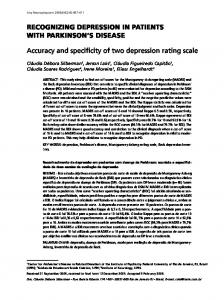
(a): An example of a closed binary silhouette contour. (b): The corresponding curvature scale space image. . . . . . . . . . . . . . . . . . . . . . . . . . . . .

5

1.2

Two fish that are distinguishable by shape. . . . . . . . . . . . . . . . . . . .

5

1.3

Two fish that are indistinguishable by shape, but unique in texture. . . . . .

6

2.1

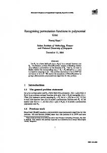
Shape contexts. (a,b) Sampled edge points of two shapes. (c) Diagram of logpolar histogram bins used in computing the shape contexts. (d-f) Example shape contexts for reference samples marked by ◦, , / in (a,b). Each shape context is a log-polar histogram of the coordinates of the rest of the point set measured using the reference point as the origin. (Dark=large value.) Note the visual similarity of the shape contexts for ◦ and , which were computed for relatively similar points on the two shapes. By contrast, the shape context for / is quite different. This figure is reprinted from from Mori et al. [65] by c 2005 IEEE. . . . . . . . . . . . . . . . . . . . . . . . . . . . . . 14 permission.

2.2

A binary image (a) with black representing ones and white representing zeros, and its distance transform (b). The “hottest” values in (b) reflect the fact that these areas are furthest from the black pixels. . . . . . . . . . . . . . . . 16

2.3

An example of a set of parabolas whose lower envelope (marked with a thicker red line) makes up a 1-D distance transform. . . . . . . . . . . . . . . . . . . 19

3.1

Sample of boundary curves. . . . . . . . . . . . . . . . . . . . . . . . . . . . . 26

3.2

(a): Gaussian smoothing process of a closed curve shown at the left most figure. (b): The corresponding curvature scale space image. . . . . . . . . . . 29

3.3

A database with 131 fish divided into 17 classes. Every row represents a class of fish (see [60].) . . . . . . . . . . . . . . . . . . . . . . . . . . . . . . . . . . 31

xi

3.4

Mirror reflection. (a): The boundary curve and its 180◦ rotation and vertical mirror transformations. (b): The corresponding CSS images. (c): The corresponding vectors r as computed by Eq. (3.9). (d): The corresponding phase-correlated vectors ˜ r.

3.5

. . . . . . . . . . . . . . . . . . . . . . . . . . . . 37

A shape database of 216 boundary curves, divided into 18 classes. Every row represents a class of object. . . . . . . . . . . . . . . . . . . . . . . . . . . . . 41

3.6

(a.): Left: A fish in database 1. Right: The corresponding CSS image, with smoothing level σ on the ordinate and contour arc length t along the abscissa. While some example CSS images in this chapter are of higher resolution for visualization purposes, the CSS images used in the experiments were typically reparameterized to have a contour length of 200 and 40 σ levels. (b): The corresponding phase-correlated marginal-sum feature vector. Each point along the abscissa represents a particular entry in the 240-D feature vector, and the correspondingly plotted height value represents the magnitude of the feature vector entry at that particular location. . . . . . . . . . . . . . . . . . 43

3.7

Matching results for a fish in database 1, using our algorithm. The top-left curve shows the input fish. The rest of the fish show the best 15 match results, ranked by their Euclidean distance to the input fish in the eigenspace subspace. The fish’s class appears as a label over each fish. . . . . . . . . . . 45

3.8

(a): An image in database 3 (‘chopper-01.gif’); (b): The standard-length contour. (c): The corresponding CSS image. (d); The corresponding feature vector: the phase-correlated marginal-sum component is shown in blue, and the row-sum is shown in green, dashed. . . . . . . . . . . . . . . . . . . . . . . 48

3.9

ROC curve for the class 0 fish shown in Figure 3.6. . . . . . . . . . . . . . . . 49

3.10 Left: Plotting the matching average for database 1 vs. the number of bases used to form the eigenspace. Right: The plot for database 2. . . . . . . . . . . 49 3.11 Left: Plotting the matching average for database 1 vs. the numbers of bases used to form the eigenspace. Solid line: raw CSS method. Dotted line: marginal-sum feature vector method. . . . . . . . . . . . . . . . . . . . . . . . 50 3.12 Rotated hammers are included in the 15 best matches, when database 2 is queried. . . . . . . . . . . . . . . . . . . . . . . . . . . . . . . . . . . . . . . . 50 3.13 Mirrored fish are included in the 15 best matches, when database 1 is queried. 51

xii

3.14 Matching results for MPEG-7 contour database, using the specialized EigenCSS method, over number of basis vectors used. Success rate at dimension 5 is 99.2%.

. . . . . . . . . . . . . . . . . . . . . . . . . . . . . . . . . . . . . . 51

3.15 Two challenging contours and their CSS images. Note that (c) and (d) would appear very similar to the basic maxima-matching method, while the marginal-sum feature can capture more information via the differences in column sums due to the different width of the CSS ‘loops’. . . . . . . . . . . . 54 3.16 Matching results on a query contour with shallow concavity.

(a.)

The

maxima-based method fails to return any correct matches. (b.) Better results from the marginal-sum feature. . . . . . . . . . . . . . . . . . . . . . . . . . . 56 4.1

Underwater video images of two species of fish. . . . . . . . . . . . . . . . . . 58

4.2

The two types of fish to be classified. . . . . . . . . . . . . . . . . . . . . . . . 60

4.3

The crosses and yellow lines in 4.3(b) are the estimated correspondences from the same-colored tree structure in 4.3(a) using the method described in this chapter. The blue circles and lines in 4.3(b) show the top shape context correspondence matches without consideration of spatial information; that is, results equivalent to employing Eq. 4.1 without the second term. Note that the yellow lines in 4.3(b) retain some spatial structure, allowing the recovery of an approximate affine warping transformation. However, the blue lines criss-cross wildly, reflecting the fact that the shape contexts were unable to determine accurate point correspondences based on SC matching costs alone. The same situation is evident in the second row; in 4.3(d), underwater plants create background clutter that generates spurious edges and throws off the shape context costs. The addition of the tree’s spatial constraints helps overcome the problem, as can be seen in 4.3(e). . . . . . . . . . . . . . . . . . 61

xiii

4.4

Edges extracted from the image by a Canny edge detector are shown in 4.4(a). 4.4(b) shows a visualization of a circular shape context histogram in red, with yellow bars representing the magnitude and direction of each bins’ counts. 4.4(c) shows the SC matching cost between the histogram from 4.4(b) and the edges of a second, differently oriented image whose edges are denoted by black dots. The costs are calculated at every pixel location in the second image and the best match (shortest Euclidean distance between histogram vectors) appears at the “hottest” spot, marked with a cross. . . . . . . . . . . 63

4.5

A diagram of the steps in the deformable template matching of a query fish image with two templates. Note how the query image warps well to template 1 but poorly to template 2. . . . . . . . . . . . . . . . . . . . . . . . . . . . . 66

4.6

Warping examples: in each row, the rightmost column shows the result of warping the leftmost column into approximate alignment with the center column images, using an affine transformation estimated from the calculated point correspondences. The first two rows show reasonable transformations (4.6(f) and 4.6(c)), while the correspondences were not recovered well in the third row example and consequently 4.6(i) is distorted. . . . . . . . . . . . . . 68

xiv

List of Algorithms 2.1

Fast distance transform algorithm pseudocode. . . . . . . . . . . . . . . . . . 20

3.1

The original CSS maxima-matching algorithm. . . . . . . . . . . . . . . . . . 30

3.2

Structure of Stage 1 Eigen-CSS processing. . . . . . . . . . . . . . . . . . . . 38

3.3

Structure of Stage 2 Eigen-CSS processing. . . . . . . . . . . . . . . . . . . . 39

4.1

Steps in deformable template matching for fish recognition. . . . . . . . . . . 62

xv

Chapter 1

Introduction 1.1

Object recognition

This thesis describes work on shape matching and object recognition. In Chapter 3, we propose a framework in two stages for a novel approach to both representing and matching the curvature scale space (CSS) features of shape silhouette contours. The results presented show this method, called Eigen-CSS, to be substantially more accurate and faster than published methods. In Chapter 4, we present a deformable template object recognition method for classifying fish species in underwater video. The two methods, Eigen-CSS shape matching and deformable template matching followed by texture-based recognition, are contrasted as complementary techniques that respectively suit the unique characteristics of two substantially different computer vision problems.

1.1.1

Motivation

A primary goal of computer vision research is to develop techniques that allow computers to recognize objects in images or video. There are numerous applications that motivate the development of object recognition methods. Some examples include: • assisting a robot to determine its topological location [78] and to perform tasks using specific items, • the navigation and targeting of aerial, aquatic or terrestrial autonomous vehicles, • industrial inspection, positioning or sorting of mechanical parts or foodstuffs,

1

CHAPTER 1. INTRODUCTION

2

• diagnostic or assistive medical applications, • interactive toys, • human motion capture [58] for movies or games, • fingerprint, facial, character and handwriting recognition, • the retrieval of multimedia from electronic databases for entertainment, science, art, business or engineering applications, • content recognition software, for example to identify copyrighted images or video posted on the internet, and • surveillance or census systems for vehicles, people or animals. Automating certain of these object recognition tasks using computer vision may yield savings across a range of areas—potential benefits could include greater efficiency, increased recognition accuracy, mitigation of human exposure to a dangerous environment, or reduction of tedious manual labor.

1.1.2

Challenges

However, object recognition is a difficult problem, especially when the basis of comparison is the performance of a human observer. Many aspects of our visual system that we take for granted are challenging to replicate mechanically; for example, adjusting to differences in the color or intensity of a scene’s illumination. Also, in addition to the powerful processing capability of the brain and optical system, humans have access to a wealth of contextual information and prior learning with which to aid their recognition decisions. Further, people have innate biological affinities for recognizing certain patterns, such as faces [70]. Because of the breadth of the problem, most computer vision object recognition methods concern themselves with limited scenarios rather than attempting to generalize to completely unconstrained vision tasks. Consequently, techniques may be predicated on assumptions about the types of images used as input—for example, the silhouette matching algorithm described in Chapter 3 requires relatively clean, closed binary contours. Or, in the case of the method for recognizing fish species described in Chapter 4, the number of species is limited to make the problem more tractable. The necessity of making these types of compromises


3

is a testament to the power of the human visual system, however it by no means diminishes the usefulness of object recognition techiques in everyday applications. A concrete example of computer vision working in tandem with human observation is computer-aided diagnosis (CAD), which refers to image analysis systems that aim to reduce the number of tumors missed by radiologists viewing x-ray images. Rather than leaving such a crucial task fully to an automated system, the computer analysis complements a doctor’s reading by flagging possible lesions, while leaving the final subjective decision to the human expert who may employ unquantifiable experience-based judgement to finally decide if a tumor is dangerous. Although the computer vision algorithms cannot currently match the performance of a human observer, the combination of doctor and automated recognition system may be better than the doctor alone [18]. Examples such as these motivate continued work on object recognition problems, since they prove the worth of such systems despite the fact that they may be forced to address a partially limited problem domain. Computer vision exploits a wide variety of methods in pursuit of object recognition [86], some of which are better suited to certain applications than others. An important factor in the success of a particular method is its suitability to the images to which it is applied. One way of ascertaining a particular vision method’s applicability to a problem setting is to examine the availability of the image characteristics on which the method relies. Features such as shape, color, texture and are utilized to different degrees by different recognition techniques, so the availability of a particular feature in an image or video strongly influences the most effective recognition method for that particular scenario. This thesis describes two methods that are tailored to the problems to which they are applied. Chapter 3 presents a technique for retrieving matching shapes from a large database of closed binary silhouette contours. In contrast, Chapter 4 details a method for texturebased recognition of nearly identically shaped fish. Figure 1.1 displays examples of two sea-creature contours whose shapes make them distinctive, despite the images’ relative simplicity. Contrast this with Figure 1.2, which shows fish with very similar silhouettes but different textures. These differences motivate the two approaches delineated in Chapters 3 and 4. While the texture comparison of Chapter 4 would be impossible to apply to the contours of Figure 1.2, the shape matching of Chapter 3 would be equally ill-suited to discriminating between the similarly shaped fish of Figure 1.3. The two methods are juxtaposed with the goal of illuminating their complementary nature. Rather than try to rank their effectiveness relative to one another, the intention is


4

to illustrate how different vision techniques are appropriate for different problem domains and to provide examples in the areas of both shape and appearance.

1.1.3

Eigen-CSS shape matching

In Chapter 3 we present a method for matching binary shape contour images. An object’s shape is a very important property when attempting visual recognition. Compared to other attributes, for example color or size, shape has the potential to discriminate and recognize a greater number of objects with better accuracy. At the same time, shape is a more amorphous concept than other properties—some of the numerous methods for categorizing objects by shape are outlined in Chapter 2. Palmer [71] describes shape as the spatial structure of an object that does not change under translation, rotation, dilation or reflection. This definition captures the idea that shape is intrinsic to an object—a square is still a square if you rotate it 45◦ and double its size. However, shearing a square distorts its 90◦ corners and renders it no longer a square. Despite this, the resulting diamond can intuitively be said to share more in shape similarity with the original square than, say, a circle. Thus shape is not a clear-cut attribute of an object; hence the multitude of ways to characterize it for computer vision applications. The Eigen-CSS shape representation is based on curvature scale space (CSS) images [61, 60], a method from the MPEG-7 standard [12]. CSS images represent the curvature zerocrossings of a contour that has been parameterized by arc length, under evolution by a Gaussian filter of gradually increasing standard deviation σ. The distance along the curve is plotted on the x-axis, while σ is plotted along the y-axis. Figure 1.1 shows a contour and its CSS image, while Figure 1.2 is an example of some shape silhouette contours. Our method matches the CSS images of contours using dimensionality reduction via principal component analysis (PCA). The feature vector employed is the concatenation of the row- and column-sums of the original CSS image. Phase correlation through Fourier transforms is used to handle CSS images’ inherent ambiguity due to varying boundary start locations. The Eigen-CSS method is shown to be as accurate as previously published approaches, while substantially faster and very simple to implement.


5

Gaussian filtering pr smoothing scale: Gaussian sigma

Curvature Scale Space image: locations of zero curvature points

path length variable t

(a)

(b)

Figure 1.1: (a): An example of a closed binary silhouette contour. (b): The corresponding curvature scale space image.

Figure 1.2: Two fish that are distinguishable by shape.

1.1.4

Deformable template matching and texture-based classification

Chapter 4 describes the recognition of fish species in frames from underwater video. Figure 1.3 shows an example of two fish to be classified. In comparison with the contours in Figure 1.2, textural appearance is the only discriminative aspect of the fish—the two species


6

classes share the same shape and color, and so cannot be grouped using these features. Instead, it is the presence of a single stripe or multiple stripes that serves to distinguish the two classes of fish. Given this difficult recognition task, we approach it as a deformable template matching problem1 , followed by the application of a supervised learning classifier. The idea is to align the fish images before classifying by texture, an approach that is shown in Chapter 4 to give a demonstrable increase in performance. The combination of shape context descriptors [8] and efficient dynamic programming-based correspondence using the distance transform [28, 30] are a novel contribution of this chapter. Shape contexts alone cannot estimate templateto-query correspondences as well as the technique employing spatial structure, because the underwater images are of very low quality. In addition, the tree structure makes the computation of globally optimal solutions possible via dynamic programming (see §2.3). Our method is motivated by ideas similar to Berg et al.’s integer quadratic programming approach [10], but is less computationally expensive.

(a) Striped Trumpeter

(b) Western Butterfish

Figure 1.3: Two fish that are indistinguishable by shape, but unique in texture. The methods described in this thesis are motivated by practical applications. Hence, due to the difficulty of unconstrained vision problems, as described above, it was necessary to simplify certain aspects of each of the problems. In the case of the contour matching in Chapter 3, the assumption of a relatively clean, closed silhouette may not be reasonable in a general, unconstrained setting. However, for applications such as industrial situations where lighting and background can be controlled, such contours can be recovered. Also, the intent of the experiments in Chapter 3 is to test the shape representation and retrieval algorithms themselves, so the assumptions of idealized input data are valid. 1

See §2.1.4, for a review of other deformable template matching techniques.


7

For the underwater recognition problem described in Chapter 4, the motivation is to reduce the time that human observers must spend watching boring underwater video footage. In this case, the method described is not fully automatic but is designed to serve as a component of a complete fish census system.

1.1.5

Outline

This thesis presents techniques for matching silhouette contours and for recognizing fish in underwater video. The former is a new method of representing and matching the CSSshape representation, called Eigen-CSS. The latter is a deformable template matching technique employing shape contexts and larger-scale spatial structure. We begin by describing previous work in Chapter 2. In Chapter 3, results are reported that show the Eigen-CSS method to be more effective and faster than previously published methods. Chapter 4 presents results that illustrate the effectiveness of the deformable template matching in improving the outcome of a difficult underwater classification problem. Finally, we conclude in Chapter 5.

Chapter 2

Previous Work This chapter contains a brief review of some of the previous work that underlies and motivates the techniques described in this thesis. While the silhouette matching of Chapter 3 and the deformable template matching of Chapter 4 draw on both some shared background and on some disparate ideas, precursor works for both methods are described together here. Since so many object recognition techniques are based on others, or are made up of combinations of previous works, it is difficult to follow a completely strict categorization when reviewing them. However, in an attempt to organize the literature review in terms of shared method characteristics, this chapter is generally laid out as follows: • Shape matching methods (§2.1) – Silhouette-based methods – Region-based methods – Skeleton-based methods – Deformable template matching – Chamfer matching and Hausdorff distance • Distance transforms (§2.2) • Dynamic programming on a tree structure (§2.3) • Support vector machines (§2.4)

8

CHAPTER 2. PREVIOUS WORK

2.1

9

Shape matching methods

The use of shape as a means towards solving computer vision problems has an extensive history. Veltkamp and Hagedoorn provided a survey of many shape matching methods [94], dividing image comparison methods into two general types: • intensity-based approaches that make use of pixel brightness information, color and texture; and • geometry-based approaches that employ the spatial configuration of features extracted from the image. The deformable template matching of Chapter 4 first makes use of geometry-based spatial configurations and finally makes a classification based on textural pixel-brightness information. In contrast, the silhouette contour matching method of Chapter 3 is concerned solely with the latter category, in that it uses no pixel intensity information and only employs features derived from a binary image contour. Within the geometry-based approaches, further divisions can be drawn among silhouettebased, region-based, and skeleton-based methods. Silhouette-based techniques are those relying solely on an object’s enclosing contour, e.g., the curvature scale space methods described in Chapter 3, or Fourier and wavelet descriptor methods. Region-based are those techniques employing information about the area inside the object’s body; for example, the moment-based methods of §2.1.2. In contrast, skeleton-based refers to techniques employing a tree-like structure based on an erosion of the original shape, such as Sebastian et al.’s shock graphs [80].

2.1.1

Silhouette-based methods

Curvature scale space The curvature scale space (CSS) image [62, 59, 61, 12], is a shape representation based on a plot of the zero-crossings of the curvature function of a closed-contour curve under evolution with a Gaussian of progressively increasing standard deviation σ. Among the attractive aspects of this shape representation are its ability to capture multi-scale shape characteristics and its effective invariance to affine transformations of the original contour. The CSS representation has been adopted as a shape descriptor in the MPEG-7 standard [60, 12]. Chapter 3 presents our improvement to the representation and matching of CSS images.


10

Curve segments Sun & Super [87] described a parts-based statistical shape classification framework in which shape classes are modeled by a set of contour segments taken from many example shapes. The algorithm matches a set of segments from an input shape with sets of class segments. A contour is broken into segments based on the location of critical points, or the extrema of the contour’s curvature function (see Eq. 3.4, p. 28). After processing for translation, rotation and scaling invariance, segments are compared to find their mean and variation with respect to a set of decorrelated basis segments, and Bayesian classifiers are used to compute the probabilities of various classes. The method is tested on the MPEG-7 database with good results, achieving 98% classification accuracy. However, the contour segment matching technique takes approximately 6 seconds per shape classification in Matlab on a 1.7 GHz machine, compared with our method of Chapter 3, which requires only 7×10−5 sec on a 2.8 GHz machine and achieves comparable matching results. Fourier and wavelet descriptors Fourier shape descriptors are features that make use of coefficients obtained by applying the Fourier transform to the parameterized function describing a shape’s boundary contour. Arbter et al. used Fourier descriptors to match 2-D silhouettes of 3-D aircraft, employing phase normalization to avoid dependence on the particular contour point chosen for silhoutte parameterization [6]. Gorman et al. [37] employed Fourier descriptors to describe curve segments and used dynamic programming to search for contour segment matches. Kunttu et al. [50] improved upon basic Fourier descriptors by applying the Fourier transform to wavelet coefficients of a shape boundary at multiple scales. A characteristic of Fourier descriptors that can cause matching difficulties is their basis on global sinusoids and their corresponding sensitivity to changes in the object boundary [72]. Wavelet descriptors [19] are a multi-resolution shape characterization that is more efficient than Fourier descriptors, as well as better at representing local features due to the improved spatial and frequency localization properties of wavelet bases.


2.1.2

11

Region-based methods

Moments Given a continuous function (or silhouette in our case) f (x, y), the (p + q)th order moment mp,q is defined as: Z

∞

Z

∞

xp y q f (x, y) dx dy.

mp,q = −∞

(2.1)

−∞

For a discrete digital image, mp,q becomes XX mp,q = xp y q f (x, y). x

(2.2)

y

These moments capture region-based, global image information. Moments, and functions of moments, were among early computer vision techniques used to characterize images for matching [42, 72]. Hu [42] described a set of moment invariants to improve upon the basic image moments; for example, the central moments µp,q (described in Eq. 3.19, p. 44), are invariant to translation. Other global object features that have been used for shape description are area, eccentricity (Eq. 3.17, p. 44), circularity (Eq. 3.20, p. 44), compactness, major axis orientation, Euler number, concavity tree, shape numbers, and algebraic moments [94]. Difficulties of moments include sensitivity to distribution of mass in the image silhouette [72]. Khotanzad and Hong [48] proposed using Zernike moments, which are the coefficients of an image expanded into orthogonal Zernike polynomial bases. In addition to the Zernike moments’ rotational invariance, they possess the desirable property of orthogonality, enabling the separation of the individual contribution of each order Zernike moment, as opposed to the partially redundant information content of regular moments. Zernike moments were found to outperform regular moments and moment invariants in a test matching images of characters.

2.1.3

Skeleton-based methods

Shock graphs Sebastian et al. [80] described a technique for matching shapes based on hierarchical skeletonlike shock graphs that represent shapes. These graphs represent the singularities of medial axis transforms, obtained by the “grassfire” evolution of shapes; the term “shock” is derived


12

from viewing these points as instabilities of wavefront propagation from the object contour inward. Each shape is thought of as a point in a shape space and the distance between two shapes is the minimum cost of the deformation taking one shape to the other. The finding of this cost is made feasible by enumerating the shock graph edits which are transitions in the partitioned, discretized shape space. The shock graph editing technique gives very good results for shape recognition, however its high computational cost makes it slow compared to other methods. Sebastian and Kimia [79] compared curve-based shape matching with a skeleton-based approach and concluded that the curve-based technique was approximately an order of magnitude faster. Although the skeleton-based method better handled shape variations such as part-rearrangement and articulation, the curve-based approach had a roughly equivalent recognition rate for other matching problems, with substantially less computational complexity.

2.1.4

Deformable template matching

The idea underlying deformable template matching is that shapes which share a general similarity may be transformed so that they deform into alignment with one another. To recover the necessary transformation, a correspondence between an unknown shape and a model must be found. After the correspondence is determined, an aligning transformation can be recovered and the degree of shape similarity can be characterized based on the magnitude of the transformation and any remaining disparity after the deformation is complete. There are several types of deformation transformations that may be employed: • rigid: a linear, non-distorting transformation consisting of rotation and translation, • affine: a linear transformation with stretching and shearing, • piecewise affine: a non-linear combination of different affine transformations for different parts of an image, • elastic: a non-linear, non-rigid deformation; for example, interpolating thin-plate splines [13]. In this case, “linear” refers to the ability to represent the transformation with a 4×4 matrix. Deformable template matching has been the subject of a considerable body of computer vision research. Fischler and Elschlager [32] presented a framework for the use of this


13

concept in computer vision and implemented shape deformation by modeling the problem as energy minimization of interconnected spring-masses. Cootes et al. [20] posited that flexible template models should only be able to deform in ways characteristic of the class of objects that they represent, and thus performed matching based on point distribution models derived from hand-picked points on example images. Amit and Kong [5] matched landmark graphs to collections of point features extracted from a target image. The types of shape variations considered were constrained by considering dynamic programming matches of decomposable subgraphs of the original template graph. Felzenszwalb [27] followed this idea by representing shapes as triangulated polygons, whose faces then form a tree whose structure can be exploited to allow efficient global optimal matches. The matching proceeds by minimizing an energy function that assigns costs based on the deformation of the triangle polygons and also incorporates a cost attracting the template boundary to locations with high image intensity gradient magnitude. The following deformable template matching techniques share several aspects: the use of a local descriptor to guide the search for correspondences between images, and a technique for recovering the correspondences themselves. Some local descriptors include scale invariant feature transform (SIFT) features [56], geometric blur [11], and shape contexts [8]. SIFT features are collections of oriented local image gradients, located at stable image scale-space extrema. Berg, Berg & Malik [10] used deformable shape matching to recognize object categories. The local descriptor employed is geometric blur, a point descriptor that consists of samples from a radially smoothed local edge image. The correspondence method used is the relatively computationally costly integer quadratic programming, formulated in a way so as to allow convenient approximation of a reasonable solution. Shape contexts Along a similar tack, Belongie et al. [8] and Mori et al. [65] also perform object recognition via shape similarity. However, the local descriptor that they use is a radial log-polar histogram of edge points dubbed the shape context. To derive correspondences, weighted bipartite matching via the Hungarian method is employed. The deformations are modeled by thin plate splines [13]. Figure 2.1 shows an example of shape edge points, a log-polar histogram, and some shape contexts. For a particular location, its shape context captures the relative spatial locations of all the edge points within the circumference of the shape context bins.


14

(a)

(b)

(c)

(d)

(e)

(f)

Figure 2.1: Shape contexts. (a,b) Sampled edge points of two shapes. (c) Diagram of logpolar histogram bins used in computing the shape contexts. (d-f) Example shape contexts for reference samples marked by ◦, , / in (a,b). Each shape context is a log-polar histogram of the coordinates of the rest of the point set measured using the reference point as the origin. (Dark=large value.) Note the visual similarity of the shape contexts for ◦ and , which were computed for relatively similar points on the two shapes. By contrast, the shape context for / is quite different. This figure is reprinted from from Mori et al. [65] by c 2005 IEEE. permission. In Chapter 4 we use generalized shape contexts, which are an extension of shape contexts that records the dominant orientation of the edge points within each histogram bin. At a point pi , the shape context is a histogram hi capturing the relative distribution of all other points such that hi (k) =

X qj ∈Q

tj , where Q = {qj 6= pi , (qj − pi ) ∈ bin(k)}

(2.3)


15

and tj is a tangent vector that is the direction of the edge at qj . Shape contexts [64, 8] have been used for a number of object recognition tasks: automatically breaking visual CAPTCHAs [66], efficient pruning of a shape database for faster matching [65], recovering 3-D human body configurations [67] and pose estimation [57]. Thayananthan et al. [89] compared shape context and chamfer matching. They concluded that the correspondences derived from shape contexts could be improved by including a “figural continuity constraint”; our combination in Chapter 4 of shape contexts and spatial distortion costs is conceptually analogous. Pictorial structures Felzenszwalb and Huttenlocher [30] present another deformable template method, motivated by Fischler and Elschlager’s original parts-based model. Objects are represented as collections of parts with individual appearance models, and the connections between parts are modeled as deformable spring-like connections. The connections are restricted to treestructured graphs so that dynamic programming can be used, along with an efficient distance transform method [28], to efficiently find globally optimal correspondences.

2.1.5

Chamfer matching and Hausdorff distance

Borgefors [14] described a matching method that finds the best fit of edge points from two images by minimizing a generalized distance between them. Image edge points are distorted by a set of parametric transformation equations, with the goal of finding a geometric distortion that brings both images into optimal position. In the hierarchical chamfer matching algorithm, a resolution pyramid reduces the computational cost of the matching. Along similar lines, the Hausdorff distance [43, 76] is a metric used to quantify the degree of resemblance between two objects represented as binary images or sets of points. The Hausdorff distance H(A, B) is a distance between two finite point sets A = {a1 , . . . , ap } and B = {b1 , . . . , bp } is defined as H(A, B) = max(h(A, B), h(B, A))

(2.4)

h(A, B) = max minka − bk

(2.5)

where

a∈A b∈B


16

and k.k is a norm on the points of A and B, such as L2 distance. The Hausdorff distance and chamfer matching are similar conceptually to binary correlation. However, they measure proximity rather than exact superposition, and hence handle real-world edge sets better [43]. One drawback of the Hausdorff distance measure is its sensitivity to outliers; consequently the term maxa∈A in Eq. 2.5 may be replaced with a quantile value1 rather than using the maximum.

2.2 2.2.1

Distance transforms Traditional binary distance transforms

25

20

15

10

5

0

(a)

(b)

Figure 2.2: A binary image (a) with black representing ones and white representing zeros, and its distance transform (b). The “hottest” values in (b) reflect the fact that these areas are furthest from the black pixels. The distance transform of a binary image encodes the distance from a particular pixel to the nearest non-zero pixel. Given a set of points P on a grid G, with P ⊆ G, the traditional distance transform associates each grid location with the distance to the nearest point in P , DP (p) = min d(p, q) q∈P

1

For example, the

1 th 2

quantile is the median.

(2.6)


17

where d(p, q) is a measure of distance between p and q, for example the L1 or L2 norm. This is a useful tool for computer vision comparison of binary images; for example, the chamfer matching and Hausdorff distance comparisons described in §2.1.5 employ distance transforms. In this case, the binary image can be thought of as a representation of a binary function, with a black or white pixel at a particular point denoting one of the function’s two possible values. The distance transforms of binary functions are real-valued functions that facilitate comparisons; as mentioned in §2.1.5, the attractive property is that the distance functions allow the measurement of proximity rather than relying on exact superposition alone.

2.2.2

Distance transforms generalized to arbitrary functions

In computer vision applications, binary images might be derived from the output of an edge or corner detector, or might represent the locations of some other feature extracted by previous processing. In other cases, rather than just indication of the presence or absence of a feature at a pixel location, there may be information about the feature “cost” available. For example, Chapter 4 describes how at each pixel location an L2 point-feature histogram matching cost is calculated. The extension of the distance transform to an arbitrary-valued function such as histogram matching costs is referred to as the generalized distance transform. Using the same notation as Eq. 2.6, let G be a grid and f : G → R an arbitrary function. Felzenszwalb and Huttenlocher [28] define the generalized distance transform of f as Df (p) = min (d(p, q) + f (q)) . q∈G

(2.7)

That is, for a point p we would like to find a point q that is both close to p and has a small value f (q). Felzenszwalb and Huttenlocher [28] outline a method that employs generalized distance transforms to minimize, in time linear in the number of pixels, cost functions having both local and spatial terms. This technique is also employed in the parts-based deformable template method of Felzenszwalb and Huttenlocher [30]. The following descriptions of the fast generalized distance transform are paraphrased from their technical report [28]. As explained below, the following method for computing the generalized distance transform has time complexity O(n) where n is the number of pixels, compared with O(n2 ) for


18

a naive algorithm, and is referred to as a fast distance transform. The fast generalized distance transform technique also has the attractive aspect that each dimension’s transform is computed separately. As well as facilitating understanding of the algorithm, this also allows the method to generalize to arbitrary dimensions [28].

2.2.3

Separable computation of multiple dimensions

For example, a two-dimensional transform may be computed by first performing 1-D transforms along each column of the grid and then performing 1-D transforms along each row of the result; in fact, while the computation cannot be done in parallel, it does not matter whether the columns or rows are transformed first. To see why, let G = {0, . . . , n − 1} × {0, . . . , m − 1} be a 2-D grid, and let f : G → R be an arbitrary function on G. The 2-D squared Euclidean distance transform of f is given by Df (x, y) = min ((x − x0 )2 + (y − y 0 )2 + f (x0 , y 0 )). 0 0 x ,y

(2.8)

Since the first term does not depend on y 0 , it can be rewritten as Df (x, y) = min ((x − x0 )2 + min ((y − y 0 )2 + f (x0 , y 0 ))), 0 0

(2.9)

= min ((x − x0 )2 + Df |x0 (y)), 0

(2.10)

x

y

x

where Df |x0 (y) is the 1-D distance transform of f restricted to the column indexed by x0 .

Hence distance transforms of arbitrary dimension can be computed via compositions of

transforms along each dimension of the underlying grid.

2.2.4

Fast generalized distance transform algorithm

The intuitive description of the fast generalized distance transform algorithm given by Felzenszwalb and Huttenlocher [28] uses a 1-D squared Euclidean distance transform computation as an example. Let f : G → R be a function on the one-dimensional grid G, with G = {0, . . . , n − 1}. Following Eq. 2.7, the squared Euclidean distance transform of f is Df (p) = min (p − q)2 + f (q) . q∈G

(2.11)


19

Figure 2.3: An example of a set of parabolas whose lower envelope (marked with a thicker red line) makes up a 1-D distance transform. Note that at each point q ∈ G the distance transform of f is bounded by a parabola rooted at (q, f (q)), as shown in Figure 2.3. There are two steps in computing the distance transform of f . First, the lower envelope of n parabolas is computed. Then, the values of Df (p) are filled in by checking the height of the lower envelope at each grid location p. Algorithm 2.1 gives pseudocode for the process [28]. The main section of the algorithm is the computation of the lower envelope. Since any two parabolas defining the distance transform intersect at one point, the horizontal intersection of the parabola coming from grid location q and the one from p can be calculated


1: 2: 3: 4: 5: 6: 7: 8: 9: 10: 11: 12: 13: 14: 15: 16: 17: 18: 19: 20: 21: 22: 23:

20

Algorithm 2.1: Fast distance transform algorithm pseudocode. k ← 0 {∗ index of rightmost parabola in lower envelope ∗} v[0] ← 0 {∗ locations of parabolas in lower envelope ∗} z[0] ← −∞ {∗ locations of boundaries between parabolas ∗} z[1] ← +∞ for q = 1 to n − 1 do {∗ compute lower envelope ∗} s ← ((f (q) + q 2 ) − (f (v[k]) + v[k]2 ))/(2q − 2v[k]) if s ≤ z[k] then k ←k−1 goto 6 else k ←k+1 v[k] ← q z[k] ← s z[k + 1] ← +∞ end if end for k←0 for q = 0 to n − 1 do {∗ fill in values of distance transform ∗} while z[k + 1] < q do k ←k+1 end while Df (q) ← ((q − v[k])2 + f (v[k])) end for

algebraically as (f (p) + p2 ) − (f (q) + q 2 )) . (2.12) 2p − 2q If q < p then the parabola coming from q is below the one coming from p to the left of s=

the intersection point s, and above it to the right of s. The lower envelope is computed by sequentially finding the lower envelope of the first q parabolas, with the parabolas ordered by their horizontal grid locations. The algorithm calculates the combinatorial structure of the lower envelope, employing two arrays to keep track of the arrangement. The horizontal grid location of the ith parabola in the lower envelope is stored in v[i]. The range in which the ith parabola is below the others is given by z[i] and z[i + 1]. The number of parabolas in the lower envelope is stored in k. When considering the parabola at q, its intersection with the parabola from v[k] is found (v[k] is the rightmost parabola in the lower envelope computed so far). There are two


21

possibilities: • the intersection is after z[k], which we recall stores the start of the range in which the parabola from v[k] is below the others, or • the intersection is before z[k]. If the intersection is after z[k], then the lower envelope is modified to show that the parabola from q is below all others starting at the intersection point s. If the intersection is before z[k], then the parabola from v[k] should not remain as part of the newly calculated lower envelope. In that case, the parabola index k is decremented to “delete” that parabola, and the procedure is repeated. The intuition for why this algorithm is linear in the number of grid locations is as follows. Each parabola is considered for addition to the lower envelope once. The addition of a single parabola may involve deleting more than one of the others, however each parabola is deleted at most once. These are steps 5–17 in Algorithm 2.1. Finally, the computation of the distance transform via sampling of the parabola lower envelope is accomplished with a single pass over the grid positions, lines 18–23 of Algorithm 2.1. Hence both sections of Algorithm 2.1 are O(n), and the overall algorithm is linear in the number of grid locations.

2.3

Dynamic programming on a tree structure

Felzenszwalb and Huttenlocher [30] describe an efficient dynamic programming method for finding the minimal value of an energy function with two terms. The following is paraphrased from their description of the algorithm. Let G be an undirected graph G = (V, E), with vertices V = {vi , . . . , vn } representing model parts and edges (vi , vj ) ∈ E for each pair of connected parts vi and vj . A configuration L = (l1 , . . . , ln ) is an instance of an object where each li specifies the location of part vertex vi . An optimal match of a model to an image is then ∗

L = arg min L

n X i=1

! mi (li ) +

X

dij (li , lj ) .

(2.13)

(vi ,vj )∈E

The first term is a function mi (li ) which measures how well a part matches the image at a particular location li . The second term dij (li , lj ) is a function measuring the amount that the model is deformed by placing vertex vi at location li and vertex vj at location lj .


22

The two keys to this method’s efficient global optimization of Eq. 2.13 are (1) that G be connected and acyclic, that is, a tree; and (2) that the relationships between parts be expressed in a form that is amenable to the efficient distance transform method described in §2.2. The algorithm for finding the optimal configuration L∗ that minimizes Eq. 2.13 proceeds as follows. Recalling that G = (V, E), let vr ∈ V be an arbitrarily chosen root vertex. Relative to vr , each vertex vi ∈ V has a depth di —the number of edges between it and vr . Vertex vi may (or may not) have children Ci which are its neighboring vertices of depth (di + 1). All vertices other than vr have a unique parent, which is the neighboring vertex of depth (di − 1). For any leaf vertex vj (that is, a vertex with no children), the optimal location lj∗ can be computed as just a function of the location of its parent vi . This is because the only edge incident to vj is (vi , vj ), thus the quality of the best location for vj given location li for vi is Bj (li ) = min (mj (lj ) + dij (li , lj )) ,

(2.14)

lj

and the best location for vj as a function of li is lj∗ (li ) = arg min (mj (lj ) + dij (li , lj )) .

(2.15)

lj

For any vertex vj other than the root vr , assume that the function Bc (lj ) is known for each child vc ∈ Cj . Then the quality of the best location for vj given a location for its parent vi is ! Bj (li ) = min mj (lj ) + dij (li , lj ) + lj

X

Bc (lj ) .

(2.16)

vc ∈Cj

Lastly, if Bc (lr ) is known for each child vc ∈ Cr of the root vr , then the best location for the root is ! lr∗ = arg min mr (lr ) + lr

X

Bc (lj ) .

(2.17)

vc ∈Cr

The recursive nature of the functions Bj (li ) allows a simple algorithm to be used. If d is the maximum depth in the tree, for each note vj with depth d compute Bj (li ) where vi is the parent of vj . Since these are all leaf nodes, the cost Bj (li ) can be computed using


23

Eq. 2.14. Then, for each node vj with depth (d − 1) compute Bj (li ), where again vi is the parent of vj . Bc (lj ) have already been computed for every child vc of vj , since the children have depth d, hence Bj (li ) can be computed using Eq. 2.16. This pattern can be repeated, decreasing the depth until the root is reached. While computing the best costs Bj , also compute the best locations of each vj as a function of its parent location. Then, compute the optimal location lr∗ for the root. Finally, the optimal configuration L∗ can be computed for all vertices by tracing backwards from the root to each leaf, since the optimal location of each vertex is known given the location of its parent, and the optimal location of each parent is known starting from the root. The time complexity of this algorithm is O(hn), as opposed to other algorithms that require O(h2 n) time, where h is the number of possible part locations and n is the number of parts. This efficiency allows the computation of globally optimal matches of model structures to images, given the conditions of a tree-structured graph and distance transformable matching function. Dynamic programming on a tree structure has also been used to optimize the calculation of stereo correspondences [93].

2.4

Support vector machines (SVMs)

Support vector machines are supervised machine learning classifiers that partition a dataset according to a maximally separating hyperplane. Burges [15] gives an overview and describes other attractive aspects of SVMs. First, support vector machine training always finds a global minimum (as opposed to neural networks for example); this guarantees there is no other point at which the objective function has a lower value. Also, SVMs have an attractive intuitive geometric interpretation. However, there are some drawbacks to SVM classification. The results are heavily dependent on the choice of kernel, and on parameter settings such as the amount to penalize a point that lies on the wrong side of a prospective separating hyperplane. How to choose the best kernel for a particular problem is still an open research problem, leaving cross-validation or trial-and-error as the best current methods. In addition, SVMs are limited in the speed and size of datasets which they can handle, due to their computational cost. Finally, there is no established way to train a multi-class SVM classifier in one step, although Allwein, Schapire and Singer [3] present a useful approach for reducing multiclass problems to binary


24

classifications, the technique we employ in the most recent version of the work described in Chapter 4.

Chapter 3

Shape Retrieval with Eigen-CSS Search 3.1

Introduction

Shape retrieval programs are comprised of two components: shape representation, and matching algorithm. Building the representation on scale space filtering and the curvature function of a closed boundary curve, curvature scale space (CSS) has been demonstrated to be a robust 2-D shape representation. The adoption of the CSS image as the default in the MPEG-7 standard [12], using a matching algorithm utilizing the contour maxima of the CSS image, makes this feature of interest perforce. In this chapter, we propose a framework in two stages for a novel approach to both representing and matching the CSS feature. Our contribution consists of three steps, each of which effects a profound speedup on CSS image matching and increase in effectiveness. Each step is a well-known technique in other domains, but the proposed concatenation of steps leads to a novel approach to this subject which captures shape information much more efficiently. Firstly, the standard algorithm for the feature involves a complicated and time-consuming search, since the zero of arc length is not known in any new contour. Here, we first obviate this search via a phase correlation transform in the spatial dimension of the CSS image. Remarkably, this step also makes the method rotation- and reflection-invariant. Then, using experience derived from medical imaging, we define a set of marginal features summarizing the transformed image. The resulting feature space is amenable to dimension reduction via subspace projection

25

CHAPTER 3. SHAPE RETRIEVAL WITH EIGEN-CSS SEARCH

26

methods, with a dramatic speedup in time, and as well orders of magnitude reduction in space. The first stage of the resultant program, using a general-purpose eigenspace, has accuracy compatible with the original program, which uses contour maxima. In the second stage, we generate specialized eigenspaces for each shape category, with little extra runtime complexity because search can still be carried out in reduced dimensionality. Results are substantially more accurate than published methods. Both methods are rotation invariant, and are simple, fast, and effective. Material from this chapter was submitted to Image and Vision Computing [23] and also published in a 2005 tech report by Drew, Lee and Rova [24]. A closed boundary curve of an object contains rich information about the object. Examining the curve, we can recognize the object shape and often identify the type of object. For example, Figure 3.1 shows the boundary curves of several objects. Although no two curves are identical, we know all curves in the same column have similar shape and they belong to the same type of object. In fact, we can name the objects as birds, camels, forks, hammers, and elephants. A computer program constructed to recognize the object shape category based on its boundary curve is useful for retrieving similar shapes that belong to the same type of object.

Figure 3.1: Sample of boundary curves.


27

Building a shape retrieval program requires two components: a shape representation, and a matching algorithm. The curvature scale space (CSS) representation [61] has been shown to be a robust shape representation. Based on the scale space filtering technique applied to the curvature of a closed boundary curve, the representation behaves well under perspective transformations of the curve. Furthermore, a small local change applied to the curve corresponds to a small local change in the representation, and the amount of change in the representation corresponds to the amount of change applied to the curve. More importantly, the representation supports retrieval of similar shape. Spurred partly by the success of the original CSS-derived shape retrieval algorithm [59], and because of the above properties, the CSS representation has been selected as the object contour-based shape descriptor for MPEG-7 [60, 12]. In this work, we propose an alternative shape retrieval algorithm for the CSS representation. The matching is carried out in the eigenspace of transformed CSS images. In spirit, then, this approach is inspired by Nayar et al.’s manifold projection scheme [68, 69] for object and pose identification based upon appearance. Here, we are interested in developing eigenspaces that are expressive of CSS images, or rather eigenvectors of more compact expressions of these images. Objects can then be identified as belonging to the most likely subspace for categories of objects. CSS images are bedevilled by an inherent ambiguity: the zero position of arc length is not determined for a new curve, compared to the model one (see Figure 3.4). As well, reflections form a problem. To handle these rotation and mirror transformations of the boundary curve, and to improve the execution speed and matching performance, we apply the Phase Correlation method [49] along the abscissa (arc length) dimension of the CSS images. This transform aligns every curve’s zero-position—the resulting curve is a new kind of CSS image. To our knowledge, this has not been done before for CSS images. We also need to compact the large amount of information in the CSS image in order to further speed up search. Motivated by the medical imaging tomographic technique of reducing dimensionality by summing, we form a new feature vector by summing separately over each of abscissa and ordinate (arc length and scale), and concatenating into a new feature vector we call the marginal-sum vector. We determined that the simplest and most successful approach was to form the set of marginal-sum vectors and apply the phase correlation transform to sums down CSS image columns. This results in a feature vector which is not only invariant to rotations (starting position on the contour) but also invariant


28

to reflections of the contour. Each of these steps is shown to result in a faster search that does not give up the expressiveness of the original CSS formulation while simplifying the search procedure considerably. This chapter is organized as follows. In §3.2 we review the CSS representation and the standard shape retrieval algorithm. Section 3.3 describes our new matching algorithm, and §3.4 reports experiment results. The advantages of the algorithm are discussed and conclusions are drawn in §3.5.

3.2 3.2.1

Synopsis of CSS Matching by Contour Maxima CSS Representation

The CSS representation [61] relies on a binary 2-D image, called the curvature scale space image, to represent the shape of a closed curve L0 parameterized by path length t L0 (t) = L0 (x(t), y(t))

(3.1)

over multiple scales (see Figure 3.2). The x dimension of the CSS image specifies the parameterized path length t of the curve and the y dimension specifies scales of the curve corresponding to the standard deviation σ of a Gaussian function 1 2 2 g(t, σ) = √ e−t /2σ . σ 2π

(3.2)

The binary CSS image is constructed by convolution of the closed curve L0 (t) by a series of Gaussians g(t, σ) with increasing σ, given by L(t, σ) = L0 (x(t), y(t)) ⊗ g(t, σ) = (X(t, σ), Y (t, σ)),

(3.3)

where ⊗ denotes a convolution operation, X(t, σ) = x(t)⊗g(t, σ), and Y (t, σ) = y(t)⊗g(t, σ). The curvature functions κ(t, σ) of the smoothed curves L(t, σ) are then calculated as κ(t, σ) =

∂X ∂ 2 Y ∂ 2 X ∂Y ∂t ∂t2 − ∂t2 ∂t . 2 ∂Y 2 3/2 ) + ( ) ] [( ∂X ∂t ∂t

(3.4)

For every zero-curvature point, i.e., κ(t, σ) = 0 and ∂κ(t, σ)/∂t 6= 0, the corresponding location (t, σ) in the binary CSS image is set to 1. The markings of the zero-curvature points form a set of contours, whose appearance captures the shape of the closed curve L0 (t). Figure 3.2 shows an example of the smoothing process of a closed boundary curve and its corresponding CSS image.


29

Gaussian filtering process

(a)

smoothing scale: Gaussian sigma

Curvature Scale Space image: locations of zero curvature points

path length variable t (b)

Figure 3.2: (a): Gaussian smoothing process of a closed curve shown at the left most figure. (b): The corresponding curvature scale space image.

3.2.2

Matching by CSS Contour Maxima

The canonical CSS-based shape retrieval algorithm [59, 60, 2] is a algorithm comparing a CSS image with a set of CSS model images, in an image database, and returning a subset of models whose appearances are similar to the image. The similarity in appearance is quantified by the cost of the match between an image and a model, which is defined as the total distance between the corresponding contour maxima in the two CSS images. A perfect match has a zero cost.


30

Algorithm 3.1: The original CSS maxima-matching algorithm.

Loop for all models Cost for model is the minimum of ( matchCSS(image, model), matchCSS(model, image), matchCSS(mirror(image), model), matchCSS(model, mirror(image))) End loop Rank models based on their costs Function matchCSS(css1, css2) Loop for all contour maximum pairs of css1 and css2 Align css1 and css2 by shifting css1 horizontally Determine cost of the match End loop Return(minimum cost among all pairs) End function

In order to find the minimum cost of the match between an image and a model, the algorithm must consider all possible ways of aligning the high-scale contour maxima from both CSS images, and compute the associated cost. For every possible candidate pair of contour maxima, there are two ways to align them: either shifting the image CSS circularly in the horizontal direction or shifting the model CSS. Because of the asymmetric treatment of the image CSS and the model CSS by the algorithm, both alignment methods must be attempted, and their associated costs must be estimated separately. Unfortunately, the above procedure fails to detect the mirror-image of the input image, even if such is in the database. Therefore, the algorithm has to repeat once again by comparing the mirrored CSS image with all the models. Finally, all costs of the match must be considered to calculate the closeness in appearance for all models. The conceptual high-level structure of the algorithm is shown as pseudocode in Algorithm 3.1.


31

Figure 3.3: A database with 131 fish divided into 17 classes. Every row represents a class of fish (see [60].)

3.2.3

Class Matching Evaluation Method

Good performance was reported when the above algorithm was evaluated for image databases [60]. As an example, Figure 3.3 shows a database of 131 fish used for evaluation. These are divided into 17 classes, (0 to 16). An image database is composed of a set of boundary curves, pre-assigned into classes based on their shapes. One of the boundary curves is used to match against the other curves stored in database, and the first 15 best matches are returned. The number of returned matches belonging to the same class as the input is divided by the number of curves in that class to obtain the performance measure of the input curve. To derive the performance measure over the class the above step is repeated for all curves in the same class. Finally, the performance measure for all classes is determined.


3.3

32

Matching by Eigen-CSS

In this section, we describe Stage 1 and Stage 2 of our shape retrieval algorithm, which again rely on CSS images to represent object shapes. However, instead of measuring similarity of two CSS images by the alignment of their contour maximum pairs, we propose conducting the matching in an eigenspace of reduced image vectors. Matching images in eigenspace has been successfully applied to facial recognition [91], by finding an eigenface basis using a principal component analysis. More generally, object model bases have been learned over different objects, poses, and illuminations by eigenspace projection [68, 69]. For our application, motivated by medical imaging tomographic applications, we convert CSS images into more compact and descriptive feature vectors we call marginal-sum vectors, which are further transformed into an eigenspace using the singular value decomposition (SVD) [36] method and truncated to just a few coefficients. In Stage 1 of our algorithm, we use a general-purpose eigenspace pertaining to the whole database. In Stage 2, we create specialized eigenspaces each pertaining to a single object class.

3.3.1

Eigenspace: PCA via SVD

Dimensionality reduction is the derivation of a set of lower-dimensional vectors from highdimensional data, where the lower-dimensional coordinates still capture the relationships inherent in the original data set. The default method of dimensionality reduction in the Eigen-CSS method, principal component analysis (PCA) [47, 92], attempts to represent a large number of high-dimensional feature vectors in a database as linear combinations of a much smaller number of basis vectors (PCA is sometimes referred to as the Karhunen-Loeve transform). In terms of storage space, this reduction is a desirable goal. For example, if there are 131 shapes in a database and the feature vectors are 244-dimensional, without dimensionality reduction it would be necessary to store 131 different 244-D vectors, one for each shape in the database. However, if the set of database feature vectors is represented well by, for example, combinations of 15 basis feature vectors, then we need only store these 15 basis vectors, along with a 15-vector of weights for each shape in the database. Without dimensionality reduction, it would be necessary to store 131 different 244-dimensional vectors; with dimensionality reduction only 15 separate 244-D vectors and 131 15-D vectors are necessary. If each vector entry is a 32-bit float, the unreduced database would require


33

4 × 244 × 131 = 127856 bytes. In contrast, the database reduced to 15 dimensions requires 4 × (15 × 244 + 15 × 131) = 22500 bytes, a savings of approximately 82%. A more severe reduction to 5 dimensions would save 94% over the space needed for the full-dimensional database. Obviously, in terms of storage, there is a good incentive to reduce the feature dimensionality. The attractive aspect of this type of dimensionality reduction is that if the bases capture a large part of the variance of the original data, this significant reduction in required storage can be achieved with little loss of matching accuracy. Using singular value decomposition to discover orthogonal bases which best capture the variance of a data set in the least squares sense is one implementation of an important mathematical technique called principal component analysis (PCA). PCA facilitates the discovery of the directions of most significant variance in a data set, and consequently allows dimensionality reduction by identifying directions which can be discarded due to insignificant sample variation along them. Two key points about PCA are (1) it is linear, and (2) it derives orthogonal bases. The former characteristic refers to the representation of features as linear combinations of a set of basis vectors, and the latter means that the bases discovered by PCA are all mutually perpendicular in a multi-dimensional sense. In contrast, independent component analysis (ICA) [44] may find non-orthogonal bases for subspace representation; other dimensionality-reduction methods such as locally linear embedding (LLE) [75] and Isomap [88] do not explicitly return basis vectors at all, although they still could be fitted into the Eigen-CSS framework. Fisher’s linear discriminant analysis (LDA) [33] is another subspace method that attempts to maximize the ratio of inter-class variance to intra-class variance. In this work, PCA is chosen because it gives good results and is simple to implement via SVD. In the Eigen-CSS method SVD is used to decompose X, a matrix of mean-subtracted feature vectors, into a set of new eigenfeatures, ordered by decreasing variance accounted for. Singular value decomposition is an efficient method for decorrelating vector information. For n column vectors x1 , x2 , ..., xn ∈ Rm , we form an m × n data matrix X of mean-subtracted vectors X = [x1 − x, x2 − x, ..., xn − x].

(3.5)

The SVD operation produces factors USV = X,

(3.6)

with orthogonal m × m matrix U of eigenfeatures, S the m × m diagonal matrix of singular


34

values, and V an m × n matrix of loadings. The column vectors of U form the basis for the eigenspace. In the new representation, vector x goes into a new coefficient m-vector u via u = UT x.

(3.7)

Since the eigenvectors are ordered by variance-accounted-for, we may often be able to reduce the dimensionality by truncating u: if the number of bases used is reduced to k where k < m, the CSS eigenspace is truncated to Rk . For any two vectors u1 and u2 , here we use a Euclidean metric (L2 norm) as our distance measure.

3.3.2

Marginal-Sum Feature Vectors

The entire CSS image can be vectorized to form a column vector xi of the input matrix X for the above SVD operation. However, such a formulation will create two problems. First, the resultant input matrix X, which is an ensemble of all the vectors xi , will be very large and lead to long execution time for the SVD operation. Second, raw CSS images may be too noisy for matching. The various parameterized curves for the type of object that we intend to retrieve have slight alternations at arbitrary locations, and the CSS contour points will be unlikely to line up in their corresponding CSS images. Matching the CSS images pixel-by-pixel may not be able to achieve the optimum result. Therefore we derive special column vectors xi , that we call marginal-sum feature vectors, from the CSS images. (We have also experimented with the use of the entire CSS image; results are reported in [24]. The present method performed better than did raw CSS image matching by Euclidean distance.) To motivate the following, consider medical imaging tomographic applications. In this situation, suppose we wish to specialize to the case of 2-D skin pathologies. Doctors often consider very simple measures of skin structures based on a few diameters across the lesion. A more complicated 3-D case might involve 2-D images formed from various 3-D directions. For our skin lesion situation, the analogue would be many 2-D x-rays perpendicular to the lesion, or in other words sums over material from a particular ray direction. The same basic idea applies: we can glean much information about structures by simply considering sets of sums across them. Here we apply this concept by treating each 2-D CSS image as a structure we wish to examine. Instead of the raw data, we consider instead the set of row-sums and set of column-sums, concatenated, as a novel feature vector. The utility of this choice is borne out by the experiments below, and in fact the new vector does seem


35

to nullify to some extent the effects of noise. For further motivation of the marginal-sum feature, see the discussion in §3.4.5. Let C(i, j) denote the pixel at the ith row and j th column of an r × c CSS image. The marginal-sum feature vector x is defined as a column vector x composed of row-sum and column-sum vectors: r sums down the rows of the CSS image, and c sums across the columns. x = [r c]T : X X X T r=[ C(i, 1), C(i, 2), ... C(i, c)] , and i

i

j

(3.9)

i

X X X T c=[ C(1, j), C(2, j), ... C(r, j)] j

(3.8)

(3.10)

j

Vector r can be interpreted as the probabilities of zero curvature points, given a point t along the parameterized closed curve, while vector c denotes the probabilities of zero curvature, given a smoothing level σ. Conceptually, we can imagine the special vector as formed by collapsing the CSS image in the y and x directions separately, precisely as in a tomographic x-ray process.

3.3.3

Phase Correlation

Clearly, a rotation transformation on a closed boundary curve translates the initial point of the parameterization process, i.e., the CSS image is circularly shifted. On the other hand, a reflection transformation reverses the direction of the parameterization process, i.e., the CSS image is mirrored. Figs. 3.4(a,b) show a 180◦ rotation and a vertical mirroring transformation of a boundary curve, along with their corresponding CSS images. These transformations pose a technical challenge to our algorithm; in particular, the vector r specified in Eq. (3.9) will be affected, but the vector c specified in Eq. (3.10) remains unchanged. Our solution to this problem is to carry out a phase correlation transform [49] on the vector r, in the same way as Fourier phase normalization has been used to eliminate starting point dependency when matching contours using Fourier Descriptors [6, 50]. This can be accomplished by converting the vector to the frequency domain, calculating the magnitude as a function of frequency, and transforming the results back to the spatial domain. The effect is translational alignment of the inverse-Fourier transformed functions. Note, however, that in carrying out this transform, we depart from a conventional CSS


36

image, now going over to a phase-correlated version which is quite different from the original. But the phase correlation is carried out only in the abscissa, path-length direction, not in the ordinate, scale dimension. In fact, we carry out the phase correlation only on vector r, not on the full CSS image, and this greatly simplifies matters. Mathematically, the phase-correlated vector ˜ r can be expressed as ˜ r = |F −1 (|F (r)|)|

(3.11)

where F denotes a 1-D Discrete Fourier Transform. Figure 3.4(c) shows the vectors r for the corresponding CSS images. In Figure 3.4(d), the phase-correlated vectors ˜ r’s are plotted— these three vectors should have the same values, since as shown below in §3.3.4, in fact Eq. (3.11) produces a feature vector invariant to rotations and reflections. Therefore, we replace the marginal-sum feature vector in Eq. (3.8) by x = [˜ r c]T

(3.12)

Notice that because of the nonlinearity of the absolute value operation, Eq. (3.11) is not equivalent to forming a 2-D CSS image which has been phase-correlated along the abscissa and then collapsed onto a row-sum. It is instead a much simpler operation.

3.3.4

Mirror reflections

A “vertical mirroring” of a contour, reflecting around the middle vertical column as in Figure 3.4(a), is effected by reversing the order of the abscissa coordinates, and hence by reversing vector r. Suppose N is the number of columns in the CSS image. Then the discrete Fourier transform Fû of the row-sum ˆr of the flipped contour Cˆ is found via P ˆ i C(i, n) = r(N +1−n) ; PN Fu = u = 1..N ; n=1 rn exp(−2πi(u − 1)(n − 1)/N ), PN ˆ Fu = n=1 r(N +1−n) exp(−2πi(u − 1)(n − 1)/N ) PN = n=1 rn exp(+2πi(u − 1)(n − 1)/N ) exp(2πi(u − 1)/N ) rˆn =

(3.13)

= conj(Fu ) exp(2πi(u − 1)/N ) Thus we have that |Fu | = |Fû | and the two transforms differ only by a phase. Therefore the feature of Eq. (3.11) is invariant to vertical mirroring. As well, clearly the sums across columns, x, are also unchanged, so the complete feature vector x is invariant.


180o rotation

37

vertical mirroring

(a)

(b)

(c)

(d)

Figure 3.4: Mirror reflection. (a): The boundary curve and its 180◦ rotation and vertical mirror transformations. (b): The corresponding CSS images. (c): The corresponding vectors r as computed by Eq. (3.9). (d): The corresponding phase-correlated vectors ˜ r. For “horizontal mirroring”, wherein the contour is inverted from top to bottom, the CSS image is unchanged except that it is reversed left-right and shifted. Thus again we have that the Fourier transform of the row-sums down the columns differ only by a phase, and ˜r


38

Algorithm 3.2: Structure of Stage 1 Eigen-CSS processing.

Obtain phase-correlated marginal-sum vector for each CSS Form input matrix for SVD Perform SVD Map each CSS into Rk eigenspace

is invariant; as well, clearly the column-sums across the rows are unchanged.

3.3.5

Algorithm Structure

We constructed two different versions of the algorithm. Stage 1 is aimed at applying the CSS image transformation and dimensional reduction scheme using a general eigenvector basis. This could be used in a situation in which categorization of classes in a target database were not available. In a second stage, however, if class metadata is available, we can further develop an eigenbasis separately for each class. Projecting onto each class provides a powerful mechanism for classifying new, test CSS images. The price for Stage 2 processing is a mild increase in complexity, as we shall see below. Stage 1: General Eigenspace Our Stage 1 shape retrieval algorithm is divided into two modules: an eigenspace construction module, and a matching module. The conceptual high-level structure of the former module is shown as pseudocode in Algorithm 3.2. Matching an image is done by computing the corresponding phase-correlated marginalsum feature vector x = [˜ r c]T , and mapping it into the Rk eigenspace. Similarity between the image and the models is measured by their Euclidean distances in the eigenspace. Stage 2: Specialized Eigenspaces If a categorization of the boundary-curve database is available, a further refinement can be carried out. For example, in the MPEG-7 shape database there are 70 classes with 20 objects each. We can form a separate eigenspace for each of these 70 categories, and then match a transformed CSS feature vector with each space separately. This turns out to be


39

Algorithm 3.3: Structure of Stage 2 Eigen-CSS processing.

Obtain phase-correlated marginal-sum vector for each CSS Form input matrix for SVD for each object category Perform multiple SVDs Map test CSS into each Rk eigenspace The eigenspace that gives the closest reconstruction of the test CSS feature vector is the best category

very effective. As well, the subspace dimensionality required is found to be very low to still produce effective categorization. In sum, the algorithm is then modified to that of Algorithm 3.3. By Parseval’s Theorem, which states that the sum of the squares of the components of a function are the same regardless of the orthonormal basis under which it is represented, the matching can in fact be carried out in the reduced, eigen-coefficient domain. We wish to characterize a good fit for a test feature vector x with the approximation x ˆ by considering the Euclidean distance kx − x ˆ k2 . Now suppose the k-vector set of coefficients in a subspace is : x ˆ =

Pk

i=1 i x i ,

where x i

is the ith eigenvector. Then our distance measure, for determining how well a test feature vector x is expressed in the eigen-subspace, is given by D2

= kx − x ˆ k2 = (x T − = x T x − k k2

Pk

T j=1 x j j )(x

−

Pk

i=1 x i i )

(3.14)

assuming the eigenvectors are orthonormal so that j ≡ x Tj x . Since the first term above is fixed, for a particular test image, we minimize distance D by simply maximizing the sum of squares of subspace coefficients . The meaning of this is that the CSS image feature vector is best represented by the subspace in which its coordinates are best mapped. The idea is similar to finding the best 2-D plane of several available to best characterize a 3-D vector: the best 2-D subspace is that for which orthogonal projection of the 3-vector produces the largest-magnitude projections. While production of the object category eigenspaces does take time offline, the runtime complexity for matching is not much increased by using a Stage 2 algorithm: For the Stage 1 algorithm, using a general basis for all shapes, suppose we make use of a K-dimensional


40

subspace representation (with K quite high, say 15). Then calculating the subspace coefficients for a new image involves K dot-products of full-size feature vectors (of size S, say). Typically, feature vectors might be of size S = 200 + s, if we use 200 contour points; and s is the number of scaling levels, minus a few (4, say) noisy levels omitted at the bottom of each CSS image. If s ' 50, we have a typical feature-vector length S = 200 + 50 − 4 = 246. Matching proceeds by forming Euclidean distances from the feature vectors for all objects in the database, for reduced K-vectors, which amounts to forming dot-products. Thus the complexity overall for both creation of the K-vector and for matching amounts to K × S + N × K multiplies, if there are N objects in the database. For the Stage 2 algorithm, with a k-vector for each subspace (say k ' 2), if there are C classes then we need to form coefficients via a length-S dot-product with k eigenvectors in each class, following by finding magnitudes in the k-space as in Eq. (3.14) above for each class. Thus the number of multiplies is C × k × S + C × k. For example, for the MPEG-7 database (below), C = 70, with 20 objects each, making N = 1400. Then with S = 246, K = 15, k = 2, the Stage 1 algorithm takes 24690 multiplies and the Stage 2 algorithm takes 34580. This amounts to only a 40% increase in complexity for matching.

3.4

Experiments and Results

The algorithms presented in §3.3 have been evaluated using three shape databases.

3.4.1

Test Data Sets

The first database used is a set of 131 fish, shown in Figure 3.3 [60]. The original boundary curves in the database have very long parameterization length, ranging from 400 to 1600 points. Here, these are re-parameterized to 200 to speed up execution time. The second database used comprises 216 shapes, divided into 18 classes: bird, bone, brick, camel, car, children, classic, elephant, face, fork, fountain, glass, heart, key, mist, ray, and turtle [81]. The original database consists of binary images in TIFF format. We extracted the boundary curves of each image and again parameterized the boundary curve to 200 points. Figure 3.5 shows the entire second database. Each row represents one class of object. (A portion of the database has been enlarged and shown in Figure 3.1.)


41

The third database is the MPEG-7 Core Experiment CE-Shape-1 closed-contour database [52]. This consists of C = 70 classes (bone, chicken, cellular ph, ...) of 20 objects each (N = 1400). Again, we made use of length-200 contours.

Figure 3.5: A shape database of 216 boundary curves, divided into 18 classes. Every row represents a class of object.

3.4.2

Implementation Details

CSS images As described in §3.2.1, we computed the CSS image of every boundary curve by smoothing it with a series of Gaussian functions, whose σ value started at 5 and was incremented by one unit until no zero curvatures remained on the smoothed curve. The small σ values (from 1 to 4), associated with fine texture irregularities of the curve, were removed from


42

the CSS image to reduce the computation error introduced by a discrete boundary curve. As a result, the y-axis (the σ axis) of a CSS image had variable length, depending on the shape of the curve, but the x-axis had its length standardized to 200, the length of the parameterized curve. In order to standardize the size of all CSS images in a database, we padded the y-axis of all CSS images to a constant length, the maximum over all images. The CSS images were used to construct the phase-correlated feature vector (Eq. (3.12)), with lengths 244, 230, and 257 for databases 1, 2, and 3 respectively. Figure 3.6 shows a typical example of a boundary curve with its corresponding CSS image and marginal-sum feature vector. General Eigenspace Grouping all phase-correlated marginal-sum vectors and forming the input matrix X (Eq. (3.5)), we built the eigen-CSS eigenspace using the first K = 15 column vectors in SVD matrix U, i.e., the eigenspace is in the subspace R15 . In [24], we analyzed the effect of selecting different number of bases and found that there was little effect on results, for K ≥ 3, with maximum average matching results at about K = 15. We also tested using raw CSS images as the vehicle for a subspace reduction [24], with of course a greatly increased execution time. We found that raw images perform substantially worse than marginal-sum feature vectors, likely because of the high noise content in CSS images. Specialized Eigenspaces As in §3.3.5, Stage 2 application of the eigenspace method involves creating a specialized eigenspace for each class in a database, and then matching against each object’s eigenspace. We found that this approach produced much better results than matching against of general eigenspace (see §3.4.4 below), and in fact better results than previously reported methods. Global parameters For the standard algorithm, a pre-processing step is typically applied to screen out contours that are most likely mismatches for the test contour, over three “global” parameters αa , αe and αc . With the subscripts i representing “image” and parameters are defined as:

m

representing “model”, the global


43

20 15 10 5

0

100

200

(a)

15

10

5

0

0

50

100

150

200

250

(b)

Figure 3.6: (a.): Left: A fish in database 1. Right: The corresponding CSS image, with smoothing level σ on the ordinate and contour arc length t along the abscissa. While some example CSS images in this chapter are of higher resolution for visualization purposes, the CSS images used in the experiments were typically reparameterized to have a contour length of 200 and 40 σ levels. (b): The corresponding phase-correlated marginal-sum feature vector. Each point along the abscissa represents a particular entry in the 240-D feature vector, and the correspondingly plotted height value represents the magnitude of the feature vector entry at that particular location. 1. Aspect ratio parameter αa : αa =

|ai − am | max (ai , am )

(3.15)

The aspect ratio is the ratio of the number of rows to the number of columns of that CSS image [62]. Since we fix the number of columns to 200, this amounts to a check on the maximum number of scaling levels (rows) in the source and target CSS images. A comparison of shape contour aspect ratios in the spatial domain, prior to CSS processing, would have more discriminative power than the aspect ratio test


44

performed on the CSS image. However, since the latter is the implementation in the method against which we are comparing [62], we follow suit and compare CSS image aspect ratios. 2. Eccentricity parameter αe : αe =

|ei − em | max (ei , em )

(3.16)

The eccentricity e, an area-based descriptor, is the ratio of maximum to minimum eigenvalues λk , r e=

λmax λmin

(3.17)

of the 2 × 2 matrix of second-order central moments of the original 2-D curve, µ2,0 µ1,1

!

µ1,1 µ0,2

(3.18)

where the central moments of a region are defined as

µp,q =

XX x

(x − x ¯)p (y − y¯)q

(3.19)

y

and (¯ x, y¯) is the region’s centroid. In fact, since the matrix is 2-D, this can easily be calculated analytically [25]. 3. and circularity parameter αc : αc =

|ci − cm | max (ci , cm )

(3.20)

Circularity c is the ratio of the square of the perimeter to the area, a contour-based parameter. In our experiments with reimplementation of the CSS maxima-matching method we followed [62] and used a threshold of 0.3 for the global parameters.


3.4.3

45

Evaluation by Class Matching

We evaluated the algorithm using the objective evaluation method described in §3.2.3. Every boundary curve in a database was matched in turn against other curves in the database and the matching percentage for a curve, the class of the curves, and the entire database were computed. For example, Figure 3.7 illustrates the matching result for a class 0 fish in database 1. The input fish is shown in the top-left hand corner with the class name labelled over the curve. The rest of the figure depicts the best 15 match results, ranked by their Euclidean distances from the input in the eigenspace subspace. Since the input fish was in the database, it was retrieved as the best matched (it was shown as the first matching result), along with 6 other class-0 fish. Because there are 8 fish in this class, the match percentage for this particular fish was 7/8 ∗ 100% = 87.5%. For all the class-0 fish, the matching average was 73%, and the matching average was 71% for the entire database 1, with no global parameters and a general eigenspace. input: 0

0

0

0

0

7

0

0

3

3

3

2

7

3

0

7

Figure 3.7: Matching results for a fish in database 1, using our algorithm. The top-left curve shows the input fish. The rest of the fish show the best 15 match results, ranked by their Euclidean distance to the input fish in the eigenspace subspace. The fish’s class appears as a label over each fish.


3.4.4

46

Results

Table 1 shows results for all methods tested. For the database shown in Figure 3.3, the matching average as defined in §3.2.3 for all classes was reported to be 76% [60]. In a best-efforts re-implementation as stated above, our figure was 72% (see the top of Table 1). However, our implementation did not test against multiple instances of the same image, since for the method proposed here we did not need to check against images with 180◦ rotation, since the method is rotation-invariant; also, we did not need to test against mirroring, since as discussed in § 3.3.4 and shown in Figure 3.4, the method presented here is reflectioninvariant. Hence we simply implemented the “original method” (see [60], pp.77-79) and not the “mirror-image extension” ([60], p.78). As well, other possible improvements mentioned were not implemented. However, we did implement the three “global parameters” recommended (see above in §3.4.2). In comparison, the Stage 1 algorithm given here also produced a 72% success rate, but with a much simpler algorithm. However, when Stage 2 was implemented, results gave a 98% success rate, using only k = 1 eigenvectors in each class, and measuring success as returning exactly the correct (one) class. Remarkably, when Stage 2 processing is adopted, matching against specialized eigenspaces and using only 2 coefficients, the method achieves 100% classification accuracy for the first two databases. For the MPEG-7 database, the third database tested, we achieved 99% accuracy using only 5 basis vectors. In comparison to previous results reported for the MPEG-7 database [52, 87], the best result reported in [52] was a matching average of 76.5%, for matches in the top 40 objects returned. Thus the Eigen-CSS Stage 2 processing, with specialized eigenspaces, surpasses that value by 16% for the data set on which we tested. Comparing to the classification error of 98% reported in [87] for a considerably more complex algorithm based on contour segments, the present method does comparably, yielding a classification error of 99.2% using only 5 basis vectors. However, the running time reported in [87] is 6 sec per classification in Matlab on a 1.7 GHz machine, whereas the present method takes only 7×10−5 sec on a 2.8 GHz machine, implying that the present method is about 5 orders of magnitude faster. (Our implementation of the original method [60] gives classification timing results about


47

104 times slower, using global parameters, on a dual 2.4 GHz machine.) While the Stage 2 algorithm does provide for multiple models, this increases discriminability without a great increase in computational matching cost.


48

240

220

200

180

160

140

120

100

80 50

100

150

(a)

200

250

300

350

250

300

350

(b)

(c) 16

14

12

10

8

6

4

2

0

20

40

60

80

100

120

140

160

180

200

(d) 240

220

220

200

200 180 180 160 160 140 140 120 120

100

100

80 50

100

150

200

(e)

250

300

80 50

100

150

200

(f)

Figure 3.8: (a): An image in database 3 (‘chopper-01.gif’); (b): The standard-length contour. (c): The corresponding CSS image. (d); The corresponding feature vector: the phasecorrelated marginal-sum component is shown in blue, and the row-sum is shown in green, dashed. (e,f): Vertical and Horizontal mirroring. Both generate the same feature vector (d).


49

1 0.9 0.8

sensitivity

0.7 0.6 0.5 0.4 0.3 0.2 0.1 0

0

0.2

0.4 0.6 1 − specificity

0.8

1

100

100

90

90

80

80 match average for database 2

match average for database 1

Figure 3.9: ROC curve for the class 0 fish shown in Figure 3.6.

70 60 50 40 30

70 60 50 40 30

20

20

10

10

0

0

20

40

60 80 number of bases used

100

120

0

0

50


200

Figure 3.10: Left: Plotting the matching average for database 1 vs. the number of bases used to form the eigenspace. Right: The plot for database 2.


50

100 90

match average for database 1

80 70 60 50 40 30 20 10 0

0

20

40


100

120

Figure 3.11: Left: Plotting the matching average for database 1 vs. the numbers of bases used to form the eigenspace. Solid line: raw CSS method. Dotted line: marginal-sum feature vector method. input: hammer

hammer

hammer

hammer

hammer

hammer

hammer

hammer

key

hammer

hammer

key

hammer

key

fountain

Bone

Figure 3.12: Rotated hammers are included in the 15 best matches, when database 2 is queried.


input: 11

11

11

11

11

11

11

0

7

14

14

14

14

14

14

11

51

Figure 3.13: Mirrored fish are included in the 15 best matches, when database 1 is queried.

100 98

Matching average

96 94 92 90 88 86 84

0

5

10 Dimension

15

20

Figure 3.14: Matching results for MPEG-7 contour database, using the specialized EigenCSS method, over number of basis vectors used. Success rate at dimension 5 is 99.2%.


52

Table 3.1: Matching averages for databases 1, 2, and 3. Algorithm

Maxima General Eigen-CSS Specialized Eigen-CSS

#Basis Vectors

Global Parameters Database 1 (Fish): 131 Objects, 17 Classes 15 objects No 15 objects 3 15 15

#Best Matches

15 objects 15 objects

No 3

1 1 top class No 2 1 top class 3 Database 2 (Sebastian et al.): 216 Objects, 18 Classes Maxima 15 objects No 15 objects 3 General Eigen-CSS 15 15 objects No 15 15 objects 3 Specialized Eigen-CSS 1 1 top class No 2 1 top class 3 Database 3 (MPEG-7): 1400 Objects, 70 Classes Maxima 15 objects No 15 objects 3 40 objects No 40 objects 3 General Eigen-CSS 15 15 objects No 15 40 objects No 15 40 objects No Specialized Eigen-CSS 1 1 top class No 2 1 top class No 5 1 top class No

Average

62 72 71 72 98 100 68 74 72 75 97 100 3 12 5 50 37 56 61 84 93 99

The standard method, “Maxima”, and the Stage 1 Eigen-CSS method both examine how many objects in the top 15 returned are in the correct class. Stage 2 “Specialized Eigen-CSS” asks which are the top classes returned. We are interested in using the fewest number of basis coefficients and fewest classes: here we report results using either only a few basis vectors, and ask for results only in the single top classification returned. The best classification error is the Specialized Eigen-CSS method, using about 5 basis vectors with a resulting accuracy of 99.2%. This compares favorably with the considerably more complex method set out in [87], with accuracy of 98% but running time 3 orders of magnitude longer.


3.4.5

53

Motivation for marginal-sum features

As shown in Figure 3.15, there are types of outlines which can differ greatly in shape yet yield similar CSS images. Because it reflects information about the whole CSS curve, the marginal-sum method is superior for matching these types of shapes than the basic maximabased method. The maxima-matching method can be altered to better handle these types of shapes via “height-adjusted matching” [60], however the advantage of the marginal-sum feature construction is that it does not require any such changes to achieve comparable results. The rate of movement of a point on a contour during evolution is proportional to the curvature value at that point. Thus there are two cases which can cause CSS ‘loops’ to become large, reaching high σ values before the zero crossings disappear: • A shallow concavity, as in Figure 3.15(a), in which case the zero crossings converge very slowly, causing a tall CSS loop as in Figure 3.15(c). • A deep concavity (section with high curvature), such as in Figure 3.15(b), in which case it takes a great deal of smoothing to make the contour convex, causing a tall CSS loop as in Figure 3.15(d). These are cases where the marginal-sum method’s ability to capture information other than solely maxima values is of benefit. Mokhtarian and Bober [60] handle this problem by selecting a new maximum for each CSS contour based on the level of smoothing at which the line segment between two zero crossings becomes straight. Without this modification, a method based solely on loop maxima would have difficulty telling the two contours apart. However, the ‘collapsing’ effect of the marginal-sum feature will yield column sums which are quite different, hopefully giving better discrimination when matching these types of contours. Anecdotally, it seems that most of the tall CSS loops formed by shallow concavities are wider than the CSS loops formed by areas of high curvature. The marginal-sum feature vector will reflect this difference, which allows it to exploit information that the maxima-based method does not. Figure 3.16 shows results which support this idea. The maxima-matching method returns only one correct match; interestingly, the query shape itself is not returned, and none of the other results are from the same class as the query contour (Figure 3.16(a)). In contrast, the marginal-sum method returns four of the eight correct class members (Figure 3.16(b)).


(a) Contour with shallow concavity

54

(b) Contour with a highly curved concavity

(c) CSS image from contour with shallow concavity

(d) CSS image from contour with high curvature

Figure 3.15: Two challenging contours and their CSS images. Note that (c) and (d) would appear very similar to the basic maxima-matching method, while the marginal-sum feature can capture more information via the differences in column sums due to the different width of the CSS ‘loops’. Also, the marginal-sum matching returns two additional long, thin objects which are from the wrong class but are good matches in terms of shape similarity. It should be noted that according to Mokhtarian and Bober [60], the maxima-matching method would return substantially better results with the height adjustment modification and use of global parameters; in our tests we did not implement the height-adjusted method but did implement the global parameters. Regardless, these results provide an interesting illustration of the


55

superiority of the unmodified marginal-sum feature and help motivate our usage.

3.5

Conclusion

The main advantages of our algorithm are simplicity and execution efficiency. As well, the method possesses the important property of rotation- and reflection-invariance, which obviates searching for multiple instances of objects. The new feature vector also effectively removes noise and produces substantively better results than raw CSS images. For Stage 1, after building the eigenspace, which has to be performed only once for a database, matching an image against the models in a database involves mapping the image to the eigenspace and calculating the distances between the image and the models in the database. There is no complicated searching, as in the canonical method [60]. With the length of the feature vector as small as 230 elements, the matching is extremely efficient. For Stage 2, wherein multiple eigenspaces are formed, the method is still efficient, and performs better than the methods reported in [52] or [87] for the MPEG-7 database. In sum, the method we present here is simple, fast, and effective.

August 6, 2004

Andy Rova

August 6, 2004

Andy Rova

Results of my implementation of Mokhtarian’s matching method on a query contour with shallow concavity: CHAPTER 3. SHAPE RETRIEVAL WITH EIGEN-CSS SEARCH

56

Results of my implementation of Mokhtarian’s matching method on a query contour with shallow concavity:

Maxima-based matching results Results of the sum-sum method(a)for the same query contour:

Results of the sum-sum method for the same query contour:

(b) Marginal-sum matching results

Figure 3.16: Matching results on a query contour with shallow concavity. (a.) The maximabased method fails to return any correct matches. (b.) Better results from the marginal-sum feature.

Chapter 4

Recognizing Fish in Underwater Video 4.1

Introduction

In this chapter, we present a deformable template object recognition method for classifying fish species in underwater video. The main contribution is the efficient combination of shape contexts with larger-scale spatial structure information, which allows acceptable estimation of point correspondences between template and test images despite missing or inaccurate edge information. Recovered point correspondences are then used to estimate transformations which are applied to align query images with a template. Finally, the warped images are classified using support vector machines (SVMs). Quantitative results are presented which verify the effectiveness of the deformable template matching. Material from this chapter was previously published by Rova, Mori and Dill [74]. Quantifying the number of fish in a local body of water is of interest for applications such as guiding fisheries regulation, evaluating the ecological impact of dams, and managing commercial fish farms. Going beyond an aggregate count of aquatic animals, information about the distribution of specific species of fish can assist biologists studying issues such as food availability and predator-prey relationships, for example between tiger sharks and dolphins [39], cormorants [41] and sea turtles [40]. Applications like these motivate the development of methods for collecting biological data underwater. Besides video, other options for automating underwater fish counting include devices

57

CHAPTER 4. RECOGNIZING FISH IN UNDERWATER VIDEO

58

employing hydro-acoustics (sonar), resistivity counters and infrared beams [17]. Of the alternatives, sonar is best suited to coarser detections such as finding shoals of fish, while resistivity and infrared counters require fish to swim through relatively narrow enclosed spaces. Underwater video is a non-intrusive method of counting fish, as well as the only one of these techniques that can classify fish by species based on textural appearance. Other attempts to visually identify fish by species rely on constrained images or shape to make distinctions [17, 53, 63]. None of these methods would work for the problem described in this chapter, where the two species of interest have very similar shapes and the environment is natural.

Figure 4.1: Underwater video images of two species of fish. The current method is to manually analyze underwater video. Using humans for this recognition and classification task is time-consuming and tedious (and may become errorprone over time as a consequence of its tedium). Hence, there is good motivation to automate the process by using computer vision. For computer vision researchers, this problem presents a number of interesting challenges. First, the complex environment confounds simpler approaches like luminance thresholding and background subtraction. Issues include shifting colors, uneven and variable illumination, among other effects of light-water interaction, and in addition our test video exhibits sediment in the water and undulating underwater plants. These factors defeat silhouette extraction and simplistic approaches such as thresholding. As mentioned in [35, 34], even the presumably easier task (compared to identifying free-swimming fish) of finding straight underwater pipelines is challenging due to sand, seaweed and the high lightattenuation factor of water. Secondly, the recognition task is non-trivial; common cues such


59

as background context, distinctive colors and unique shapes are absent. Figure 4.2 shows examples of the two species of fish between which we attempt to discriminate. Finally, the fish appear in a variety of scales, orientations, and body poses, all factors that complicate recognition. We approach this task as a deformable template matching problem followed by the application of a supervised learning classifier. Aligning the images before classifying by appearance provides a demonstrable increase in performance. A primary contribution of this chapter is the novel combination of shape context descriptors [8] with efficient dynamic programming-based correspondence using the distance transform [28, 30] for deformable template matching. This allows the estimation of template-to-query correspondences which would not be possible using shape contexts alone because of the low quality of the underwater video images. Tree-structured dynamic programming and fast distance transform techniques from [30] make it computationally feasible to simultaneously consider both shape context matching costs and points’ spatial relationships, and to find a globally optimum correspondence. Our method recovers correspondences in low-quality images that lack distinctive or stable features; it is similarly motivated but computationally cheaper than the IQP approach in [10].

4.1.1

Previous Work

The idea of deformable template matching has deep roots within the computer vision community. Fischler and Elschlager [32] developed a technique based on energy minimization in a mass-spring model. Grenander et al. [38] developed these ideas in a probabilistic setting. Yuille [97] developed another variant of the deformable template concept by means of fitting hand-crafted parametrized models, e.g., for eyes, in the image domain using gradient descent. Other approaches in this vein [51, 20] first attempt to find correspondences between a pair of images prior to an appearance-based comparison, as we do in this chapter. Recent years have seen the emergence of part-based models approaches [56, 31, 22, 4] that characterize appearance using a collection of local image patches selected by interest point operators. Shape information is encoded via spatial relationships between the local patches. The locations for the local patches are selected with various interest point operators, and are represented either as raw pixel values [31] or histograms of image gradients [56, 22], termed SIFT descriptors (Scale Invariant Feature Transform). However, for our problem interest


60

point operators would likely not be successful due to the lack of distinctive and stable image features in underwater video. Images of a constrained environment, for example from a glass-walled fish ladder, are used in other underwater fish data-analyses such as shape-based classification [53] or counting after background-subtraction [63]. Other methods use stereo cameras to estimate traits such as fish mass [90], employ special devices through which fish must swim to generate a silhouette for shape classification [17], or utilize color for fish recognition [85]. Undersea animals are detected and tracked in a natural setting in [95], however identification is not performed.

4.2

Approach

(a) Striped Trumpeter

(b) Western Butterfish

Figure 4.2: The two types of fish to be classified. Our goal is to distinguish between the fish species shown in Figure 4.2. The Striped Trumpeter (Figure 4.2(a)), has multiple horizontal markings while the Western Butterfish (Figure 4.2(b)) sports a single bold stripe. Since the images’ color information is dominated by the water’s hue, color is not useful to differentiate these fish types. Shape also provides little discernement, so we will focus on texture-based classification. We use deformable template matching to align template images and query images in an attempt to improve the performance of such a texture-based classifier, whose results are sensitive to pixel alignment. The subsequent sections describe the details of this approach; a condensed version of the various steps is laid out in Algorithm 4.1.


(a) original MST

(c) another MST

61

(b) estimated correspondences

(d) edges in query image

(e) estimated correspondences

Figure 4.3: The crosses and yellow lines in 4.3(b) are the estimated correspondences from the same-colored tree structure in 4.3(a) using the method described in this chapter. The blue circles and lines in 4.3(b) show the top shape context correspondence matches without consideration of spatial information; that is, results equivalent to employing Eq. 4.1 without the second term. Note that the yellow lines in 4.3(b) retain some spatial structure, allowing the recovery of an approximate affine warping transformation. However, the blue lines crisscross wildly, reflecting the fact that the shape contexts were unable to determine accurate point correspondences based on SC matching costs alone. The same situation is evident in the second row; in 4.3(d), underwater plants create background clutter that generates spurious edges and throws off the shape context costs. The addition of the tree’s spatial constraints helps overcome the problem, as can be seen in 4.3(e).

4.2.1

Model generation

The following steps are repeated for each of the two classes. First, a template image representative of the current fish class is chosen, e.g., Figure 4.2(a) or Figure 4.2(b). A set of edge points similar to Figure 4.4(a) are extracted from the template using Canny edge detection. Next, a subset of 100 template edges is randomly chosen from the set of edge points. The size of this subset was chosen empirically based on our previously fixed image size. The edge subset is then connected into a minimum spanning tree (MST) using Prim’s algorithm [21]. An example of a template overlaid with a MST is shown in Figure 4.3(a).


62

Algorithm 4.1: Steps in deformable template matching for fish recognition.

Generate tree-structured template models Iteratively estimate transformations from query image to the template Filter and sum the warped query images into feature vectors Classify via SVMs

Using tree-structured models provides spatial coherence among point correspondences and allows efficient global optimization of template-query matches via dynamic programming. These model trees are stored and reused for the remainder of the matching process. Finding the best match of a template tree model in a query image will be phrased as an optimization problem with two cost terms to be minimized. As described by Felzenszwalb and Huttenlocher [30]1 , if a tree has n vertices {v1 , . . . , vn } and an edge (vi , vj ) ∈ E for each pair of connected vertices, then a configuration L = (l1 , . . . , ln ) gives an instance of an object, where each li specifies the location of part vi . Then, the best match of a model to a query is ∗

L = arg min L

n X i=1

! mi (li ) +

X

dij (li , lj )

(4.1)

(vi ,vj )∈E

where mi (li ) is a matching cost between features in the model and query image at location li , and dij (li , lj ) is the amount that model edge (vi , vj ) is changed when vertex vi is located at li and vj is placed at lj . In our method, mi (li ) will be the shape context matching cost defined in §4.2.2, and dij (li , lj ) = k(lj − li ) − (ljm − lim )k2 , with lkm denoting the location of vertex vk in the model tree. This means that the best set of point correspondence mappings from the template into the query are those that minimize the total shape context matching cost and at the same time least alter the relative spatial locations of vertices which are neighbors in the model tree. 1

Also see Chapter 2, §2.3.


4.2.2

63

Deformable template matching

For the deformable template matching we combine the strengths of shape context descriptors [8] with the distance transform methods of [28, 30]. Rather than matching a set of edge points in the model image with another set of edge points in the query image, we search every pixel location in the query image and thus find a global optimum match for the model tree. Shape contexts Our method employs shape contexts as image features because they are well-suited to capturing large-scale spatial information in images exhibiting sparse edges, a common characteristic of our underwater images.

(a) Detected edges

(b) A shape context

(c) Shape context matching costs

Figure 4.4: Edges extracted from the image by a Canny edge detector are shown in 4.4(a). 4.4(b) shows a visualization of a circular shape context histogram in red, with yellow bars representing the magnitude and direction of each bins’ counts. 4.4(c) shows the SC matching cost between the histogram from 4.4(b) and the edges of a second, differently oriented image whose edges are denoted by black dots. The costs are calculated at every pixel location in the second image and the best match (shortest Euclidean distance between histogram vectors) appears at the “hottest” spot, marked with a cross. Shape contexts [8] (SCs) are coarse radial histograms of image edge points. For a particular location, its shape context captures the relative spatial locations of all the edge points within the circumference of the shape context bins. In this work we use generalized shape contexts [65] which capture the dominant orientation of edges in each bin, rather than just the point counts. For a point pi , the shape context is a histogram hi capturing the relative distribution of all other points such that hi (k) =

X qj ∈Q

tj , where Q = {qj 6= pi , (qj − pi ) ∈ bin(k)}

(4.2)


64

and tj is a tangent vector that is the direction of the edge at qj . Figs. 4.4(a) and 4.4(b) show a visualization of edge points and a shape context. When comparing two shape contexts, we treat them as feature vectors and compute the L2 distance between them. This distance is referred to as the shape context matching cost; in our method, this is the first minimization term mi (li ) in Eq. (4.1). After a MST is constructed in the template image, shape contexts are calculated at each of the points which make up the vertices of the model tree, and these will be matched with shape contexts computed at every pixel location in the query image. Although SC histograms are only computed at a subset of template edge locations, all of the edge points which were initially output by the Canny detector are eligible to be counted by any SCs which encompass them. Distance transforms Distance transforms and dynamic programming on a tree structure [28, 30] make it computationally feasible to find globally optimal correspondences between the template model and an unknown query image, a situation for which the methods of [8, 10] are ineffective or intractable. In particular, the distance transform method can find the global optimum of Eq. (4.1) in time O(hn), where h is the number of pixels and n is the number of nodes in the tree. This allows efficient computation of dij (li , lj ) in Eq. (4.1) (see §2.2). Dynamic programming for efficient minimization The techniques of [30] are employed to find L∗ from Eq. (4.1)—the globally optimum configuration of a template model tree in the query image (see §2.3). Two key aspects of this approach make the global optimization of Eq. 4.1 computationally tractable. First, the use of a tree structure to capture the spatial relationships allows the use of dynamic programming. Secondly, the accompanying restriction that parts have a pairwise relationship with one another allows the use of generalized distance transforms. These two techniques greatly increase the efficiency of the correspondence computations, and allow globally optimal solutions to be found.


65

Iterative warping From the template-to-query correspondence estimates, a least-squares affine transformation from the query to the template can be derived. The use of affine transformations is justified since the fish are relatively flat, and since in practice the video sequence usually contained at least one side-on image of each fish. This transformation is then applied to the edge points from the query image, shape contexts are recomputed everywhere in the query image, and the correspondence process is repeated. For our experiments, a maximum of 4 iterations were performed; if a reasonable affine transformation is not found, the iterative warping process aborts. After the iterative transformation of the query edge points, the complete estimated transformation is applied to the query image. Figure 4.6 shows some examples of warped images.

4.2.3

Texture-based classification

Since the fish are the same shape but have different markings, we employ a texture-based classification method. Once the query images have been transformed into estimated alignment with the template they are processed to extract texture properties. First, each image is convolved with a 3-pixel-tall vertical central difference kernel. The motivation for vertical derivative filtering is that after successful warping, the vertical direction captures the most image information. Next, the filter response is half-wave rectified to avoid cancellation during subsequent spatial aggregation. Each half-wave component of the filter response is summed into 7-pixel square sections. Finally, all of the combined filter responses are concatenated into a feature vector as input for a support vector machine (SVM) classifier. SVMs are binary classifiers. However, in our method there are two templates, one for each type of fish, and each query image is warped to both templates. This means that we have two SVMs whose outputs need to be combined to get a final classification decision. Our situation is a simplified version of the multi-SVM problem of [3]. If both SVMs agree on a classification decision, then all is well. If the two SVMs assert opposite classifications, then the decision of the SVM with the greater absolute distance to its separating hyperplane is taken to be the true one.


template 1

query warped to template 1

66

filter responses SVM

query image

find correspondences and warp find correspondences and warp

Classification decision

SVM

template 2

query warped to template 2

filter responses

Figure 4.5: A diagram of the steps in the deformable template matching of a query fish image with two templates. Note how the query image warps well to template 1 but poorly to template 2.

4.3

Results

The steps described in §4.2—tree-structured model generation, point-correspondence estimation, iterative warping and SVM texture classification—were implemented in Matlab and tested on a set of manually cropped underwater video images of two fish species. The diagram in Figure 4.2.3 shows the sequence of steps followed to compare a query image with two templates. We used svmLight [46] for SVM classification. For both species of fish being classified 160 images were manually cropped from frames of underwater video. In these 320 images, the fish appear at different angular poses although all of their heads face the right. All images were converted to grayscale, de-interlaced and resized to 50 × 100 pixels,


67

Table 4.1: Results of SVM classification. SVM kernel linear polynomial

unwarped 84% 81%

warped 90% 86%

empirically chosen based on the size of the majority of fish in the images. 8-fold cross validation on a training set consisting of half the image data was used to select the best SVM kernels and parameters. SVMs with these attributes were then constructed for the entire training set. The results of running these SVMs on the set of test images are reported in Table 4.1. The basis of comparison is the accuracies of SVMs trained on texture features from the original, unwarped images. For both the linear and polynomial SVM kernels, warping the images into alignment with a template prior to classification improved the classification accuracy, in the best case by up to 6% (90% versus 84%).

4.4

Conclusion

This work describes a novel combination of two existing techniques—shape contexts and efficient dynamic programming-based correspondence using the distance transform—applied to classifying fish by textural appearance in underwater video. In feature-poor underwater video data, this method is able to effectively deform objects into alignment. Previous methods, such as the linear assignment problem (used in [8]) or IQP (used in [10]), would be ineffective or computationally intractable in this setting. In addition, our work goes beyond previous tracking and counting methods by classifying fishes’ species based on appearance. The motivation for the choice of the particular techniques described here is the uniqueness of this recognition problem. Compared to other computer vision tasks, for these images it is difficult to exploit useful cues like background, color and shape. These difficulties, combined with others such as low resolution, inspired the adoption of the particular methods we have described. Other methods which may be effective in different recognition problems are not necessarily suited to the task of recognizing fish in underwater video. In experiments on a dataset of fish images, we have demonstrated quantitatively the improvement in classification accuracy that can be attained by using deformable template


68

matching to align objects prior to appearance-based recognition. We used an SVM on texture descriptors to perform classification, and obtained improvements in classification accuracy of up to 6% (90% versus 84%) by running deformable template matching prior to recognition. As future work, we are developing a preprocessing and tracking component that will output cropped fish images to be classified using the method described in this chapter. The goal is a complete system that automatically detects, tracks, counts and classifies fish in underwater video, without requiring manual cropping of fish images.

(a) test image

(b) template

(c) warped test image

(d) test image

(e) template

(f) warped test image

(g) test image

(h) template

(i) warped test image

Figure 4.6: Warping examples: in each row, the rightmost column shows the result of warping the leftmost column into approximate alignment with the center column images, using an affine transformation estimated from the calculated point correspondences. The first two rows show reasonable transformations (4.6(f) and 4.6(c)), while the correspondences were not recovered well in the third row example and consequently 4.6(i) is distorted.

Chapter 5

Conclusion 5.1

Contributions

This thesis presents two methods of practical use for shape matching and object recognition. First, the Eigen-CSS shape retrieval method described in Chapter 3 is a novel technique that achieves accuracy for multiple databases equivalent to previously published methods, while being orders of magnitude faster and significantly simpler to implement. Compared with other contour-based shape matching techniques, it outperforms Fourier and wavelet descriptors, is computationally cheaper than shock graph skeleton and curve segment matching methods while giving comparable results, and is simpler to implement and outperforms the canonical CSS maxima-matching algorithm. While these results are based on the performance of the Eigen-CSS algorithm on three particular shape databases, in each case our method outperformed our implementation of the canonical CSS maxima-matching method. Second, Chapter 4 demonstrates a deformable matching technique whose main contribution is the efficient combination of shape contexts with larger-scale spatial structure information, thereby allowing acceptable estimation of point correspondences between template and test images despite missing or inaccurate edge information. The use of shape contexts is suited to the sometimes sparse-edged underwater images, in which local features such as SIFT [56] would likely perform poorly. Further, the usage of fast distance transforms and tree-structured dynamic programming allow globally optimal correspondences to be computed efficiently compared to other methods for this type of problem. Contrasted with geometric blur and IQP [10], or with shape contexts and linear assignment [8], our method is simpler and computationally cheaper, while still quantitatively improving the texture 69

CHAPTER 5. CONCLUSION

70

classification results in the presented experiments. In experiments with hand-cropped fish images, the deformable template matching improved the accuracy of fish classification by 6%.

5.2

Future work

The Eigen-CSS method has been extended to 3-D objects [55]. Other work could include the substitution of different dimensionality reduction techniques, or the usage of this method as the back end of a system that automatically extracts contours from real images. In this thesis we have demonstrated that it is possible to accurately classify fish species given a set of cropped images. Completing a fully-automated system requires a more effective preprocessing method to generate higher-quality candidates for the warping and classification process. This could involve implementing a more sophisticated detector, or obtaining higher-quality underwater video data. We experimented with a variety of combinations of tracking and motion detection, including background subtraction and color space analysis. Comparisons with hand-labeled ground truth underscored the difficulty of the problem. Because of this, we believe other useful directions may include placing stereo cameras underwater to capture depth information, or the use of other sensing modalities such as sonar to provide localization cues for the initial cropping of fish candidates from the video frames. The recognition method here could even serve as an analysis component of a system of remote robotic cameras such as those described by Song and Goldberg [83]. For example, the Automated Collaborative Observatory for Natural Environments (ACONE) system [1, 73] under development by researchers from Texas A&M, UC Berkeley and Cornell automatically captures video of birds, but does not currently perform automatic identification. Research on automatic monitoring of animal behavior is also being done by Balch et al. [7] and Belongie et al. [9]. Another point to note regarding the deformable template matching method described in this thesis is that the matching cost currently only consists of the shape context histogram similarity match. An option for extending the method that might have the potential for generalization to a broader range of recognition problems would be the addition of an appearance-similarity measure into the matching cost. For example, the correlation score of a local appearance window around a point could be balanced with the shape context score. This addition would be trivial since the rest of the algorithm would remain unaltered.

CHAPTER 5. CONCLUSION

5.3

71

Conclusion

This thesis presents two complementary computer vision methods for shape matching and object recognition. The first approach, Eigen-CSS shape matching, is concerned with the representation and matching of binary silhouette contours of objects. In contrast, the subsequent deformable template texture-classification method recognizes similarly-shaped fish that are distinguished by their surface markings. While neither approach would apply well to the data set used to test the other, when applied to the specific applications for which they were intended our experiments demonstrate an improvement in performance in both cases. Matching binary shape contours and classifying fish in underwater video are both tasks that the human visual system performs very accurately. However, over large time frames these jobs can also become tedious chores for people, and thus are good candidates for automation with computer vision. In the case of the Eigen-CSS method, the experiments were restricted to matching clean binary contours, with the understanding that these have been provided by some previous processing method. Although in some cases it may be difficult to obtain such contours from real-world images, once they are provided the method works well. The Eigen-CSS approach is also efficient, and the use of subspace decomposition and feature-summation are important steps in reducing storage and computational requirements. In Chapter 4, recognizing fish in underwater video via deformable template textureclassification was shown to be accurate, provided a reasonably cropped set of candidate fish images are provided. For this method, the greatest improvement in results would follow from better detection of fish within the video frames. Whether through higher-quality video or feedback from external sensors, well-localized fish candidates within a frame image are a key component that would allow the extension of this thesis work into a fully-automated system. The method described in Chapter 4 is also computationally efficient; two important aspects of this section are the use of fast distance transforms and tree-structured dynamic programming. These techniques allow the global optimization of a two-term correspondencematching function in time linear in the number of pixels, as opposed to the quadratic complexity of a naive algorithm. In sum, the two approaches described here are examples of shape matching and object recognition which illustrate the importance of choosing computer vision methods to complement particular problem domains and the unique data at hand.

Bibliography [1] http://www.c-o-n-e.org/acone/. [2] S. Abbasi and F. Mokhtarian. Affine-similar shape retrieval: Application to multi-view 3-D object recognition. IEEE Transactions on Image Processing, 10:131–139, 2001. [3] E.L. Allwein, R.E. Schapire, and Y. Singer. Reducing multiclass to binary: A unifying approach for margin classifiers. In Proceedings of the International Conference on Machine Learning (ICML ’00), pages 9–16, 2000. [4] Y. Amit, D. Geman, and K. Wilder. Joint induction of shape features and tree classifiers. IEEE Transactions on Pattern Analysis and Machine Intelligence, 19(11):1300– 1305, November 1997. [5] Yali Amit and Augustine Kong. Graphical templates for model registration. IEEE Transactions on Pattern Analysis and Machine Intelligence, 16(3):225–236, 1996. [6] K. Arbter, W.E. Snyder, H. Burkhardt, and G. Hirzinger. Application of affine invariant Fourier descriptors to recognition of 3-D objects. IEEE Transactions on Pattern Analysis and Machine Intelligence, 12:640–647, 1990. [7] T. Balch, Z. Khan, and M. Veloso. Automatically tracking and analyzing the behavior of live insect colonies. In Autonomous Agents, 2001. [8] S. Belongie, J. Malik, and J. Puzicha. Shape matching and object recognition using shape contexts. IEEE Transactions on Pattern Analysis and Machine Intelligence, 24(4):509–522, 2002. [9] Serge Belongie, Kristin Branson, Piotr Dollár, and Vincent Rabaud. Monitoring animal behavior in the smart vivarium. In Monitoring Behavior 2005, 5th International Conference on Methods and Techniques in Behavioral Research, 2005. [10] A.C. Berg, T.L. Berg, and J. Malik. Shape matching and object recognition using low distortion correspondences. In IEEE Computer Society Conference on Computer Vision and Pattern Recognition (CVPR ’05), pages 26–33. IEEE Computer Society, 2005.

72

BIBLIOGRAPHY

73

[11] A.C. Berg and J. Malik. Geometric blur for template matching. In IEEE Computer Society Conference on Computer Vision and Pattern Recognition (CVPR ’04), pages 607–614. IEEE Computer Society, 2004. [12] Miroslaw Bober. MPEG-7 visual shape descriptors. IEEE Transactions on Circuits and Systems for Video Technology, 11(6):716–719, June 2001. [13] F.L. Bookstein. Principal warps: thin-plate splines and decomposition of deformations. IEEE Transactions on Pattern Analysis and Machine Intelligence, 11(6):567–585, June 1989. [14] Gunilla Borgefors. Hierarchical chamfer matching: a parametric edge matching algorithm. IEEE Transactions on Pattern Analysis and Machine Intelligence, 10(6):849– 865, November 1988. [15] Christopher J.C. Burges. A tutorial on support vector machines for pattern recognition. Data Mining and Knowledge Discovery, 2:121–167, 1998. [16] H. Byun and S.-W. Lee. Applications of support vector machines for pattern recognition: a survey. In S.-W. Lee and A. Verri, editors, Pattern Recognition with Support Vector Machines: First International Workshop (SVM ’02), volume 2388/2002, pages 213–237. Springer, August 10 2002. [17] S. Cadieux, F. Lalonde, and F. Michaud. Intelligent system for automated fish sorting and counting. In Proceedings of the 2000 IEEE/RSJ International Conference on Intelligent Robots and Systems, 2000. [18] Heang-Ping Chan, Kunio Doi, Simranjit Galhotra, Carl J. Vyborny, Heber MacMahon, and Peter M. Jokich. Image feature analysis and computer-aided diagnosis in digital radiography. I. Automated detection of microcalcifications in mammography. Medical Physics, 14(4):538–548, 1987. [19] Gene C.-H. Chuang and C.-C. Jay Kuo. Wavelet descriptor of planar curves: theory and applications. IEEE Transactions on Image Processing, 5(1):56–70, January 1996. [20] T.F. Cootes, D. Cooper, C.J. Taylor, and J. Graham. Active shape models – their training and application. Computer Vision and Image Understanding, 61(1):38–59, January 1995. [21] T.H. Cormen, C.E. Leiserson, R.L. Rivest, and C. Stein. Introduction To Algorithms. McGraw-Hill, 2nd edition, 2002. [22] Gyuri Dorkó and Cordelia Schmid. Selection of scale-invariant parts for object class recognition. In International Conference on Computer Vision, volume 1, pages 634–640, 2003.

BIBLIOGRAPHY

74

[23] M. S. Drew, T. K. Lee, and A. Rova. Shape retrieval with eigen-CSS search. In submission to Image and Vision Computing, 2006. [24] Mark S. Drew, Tim K. Lee, and Andrew Rova. Shape retrieval with eigen-CSS search. Technical Report TR 2005-7, Simon Fraser University, 2005. http://fas.sfu.ca/ pub/cs/TR/2005/CMPT2005-07.pdf. [25] M.S. Drew, Z.-N. Li, and Z. Tauber. Illumination color covariant locale-based visual object retrieval. Pattern Recognition, 35(8):1687–1704, 2002. [26] Fiona F. Evans. Detecting fish in underwater video using the EM algorithm. In Proceedings of the 2003 International Conference on Image Processing (ICIP ’03), pages 1029–1032, 2003. [27] Pedro F. Felzenszwalb. Representation and detection of deformable shapes. IEEE Transactions on Pattern Analysis and Machine Intelligence, 27(2):208–220, February 2005. [28] Pedro F. Felzenszwalb and Daniel P. Huttenlocher. Distance transforms of sampled functions. Technical Report TR2004-1963, Cornell University, 2004. http://people. cs.uchicago.edu/∼pff/papers/dt.pdf. [29] P.F. Felzenszwalb and D.P. Huttenlocher. Efficient matching of pictorial structures. In IEEE Computer Society Conference on Computer Vision and Pattern Recognition (CVPR ’05), pages 66–73. IEEE Computer Society, 2000. [30] P.F. Felzenszwalb and D.P. Huttenlocher. Pictorial structures for object recognition. International Journal of Computer Vision, 61(1):55–79, 2005. [31] R. Fergus, P. Perona, and A. Zisserman. Object class recognition by unsupervised scale-invariant learning. In Proceedings of the IEEE Conference on Computer Vision and Pattern Recognition (CVPR ’03), volume 2, pages 264–271, 2003. [32] M. Fischler and R. Elschlager. The representation and matching of pictorial structures. IEEE Transactions on Computers, C-22(1):67–92, 1973. [33] R.A. Fisher. The use of multiple measurements in taxonomic problems. Annals of Eugenics, 7:179–188, 1936. [34] Gian Luca Foresti. A hierarchical classification system for object recognition in underwater environments. IEEE Journal of Oceanic Engineeering, 27(1):66–78, 2002. [35] G.L. Foresti and S. Gentili. A vision based system for object detection in underwater images. International Journal of Pattern Recognition and Artificial Intelligence, 14(2):167–188, 2000. [36] G.H. Golub and C. Reinsch. Singular value decomposition and least squares solutions. Numerische Mathematik, 14(5):403–420, 1970.

BIBLIOGRAPHY

75

[37] John W. Gorman, O. Robert Mitchell, and Frank P. Kuhl. Partial shape recognition using dynamic programming. IEEE Transactions on Pattern Analysis and Machine Intelligence, 10(2):257–266, March 1988. [38] U. Grenander, Y. Chow, and D.M. Keenan. HANDS: A Pattern Theoretic Study Of Biological Shapes. Springer, 1991. [39] Michael R. Heithaus and Lawrence M. Dill. Food availability and tiger shark predation risk influence bottlenose dolphin habitat use. Ecology, 83(2):480–491, 2002. [40] Michael R. Heithaus, Alejandro Frid, Aaron J. Wirsing, Lars Bejder, and Lawrence M. Dill. Biology of sea turtles under risk from tiger sharks at a foraging ground. Marine Ecology Progress Series, 288:285–294, 2005. [41] M.R. Heithaus. Habitat use and group size of pied cormorants (phalacrocorax varius) in a seagrass ecosystem: possible effects of food abundance and predation risk. Marine Biology, 147:27–35, 2005. [42] Ming-Kuei Hu. Visual pattern recognition by moment invariants. IRE Transactions on Information Theory, pages 179–187, February 1962. [43] Daniel P. Huttenlocher, Gregory A. Klanderman, and William J. Rucklidge. Comparing images using the Hausdorff distance. IEEE Transactions on Pattern Analysis and Machine Intelligence, 15(9):850–863, September 1993. [44] Aapo Hyvärinen and Erkki Oja. Independent component analysis: algorithms and applications. Neural Networks, 13:411–430, 2000. [45] Anil K. Jain, Yu Zhong, and Sridhar Lakshmanan. Object matching using deformable templates. IEEE Transactions on Pattern Analysis and Machine Intelligence, 18(3):267–278, March 1996. [46] T. Joachims. Advances in Kernel Methods–Support Vector Learning, chapter 11: Making Large-Scale SVM Learning Practical. MIT-Press, 1999. [47] I.T. Jolliffe. Principal Component Analysis. Springer, 2nd edition, 2002. [48] Alireza Khotanzad and Yaw Hua Hong. Invariant image recognition by Zernike moments. IEEE Transactions on Pattern Analysis and Machine Intelligence, 12(5):489– 497, May 1990. [49] C.D. Kuglin and D.C. Hines. The phase correlation image alignment method. In International Conference on Cybernetics and Society, pages 163–165, 1975. [50] I. Kunttu, L. Lepistö, J. Rauhamaa, and A. Visa. Multiscale Fourier descriptor for shape classification. In Proceedings of the 12th International Conference on Image Analysis (ICIA ’03), pages 536–541, 2003.

BIBLIOGRAPHY

76

[51] M. Lades, C.C. Vorbr¨ uggen, J. Buhmann, J. Lange, C. von der Malsburg, R.P. Wurtz, and W. Konen. Distortion invariant object recognition in the dynamic link architecture. IEEE Transactions on Computers, 42(3):300–311, March 1993. [52] L.J. Latecki, R. Lakämper, and U. Eckhardt. Shape descriptors for non-rigid shapes with a single closed contour. In IEEE Computer Society Conference on Computer Vision and Pattern Recognition (CVPR ’00), pages 1424–1429. IEEE Computer Society, 2000. [53] D.J. Lee, S. Redd, R. Schoenberger, X. Xu, and P. Zhan. An automated fish species classification and migration monitoring system. In Proceedings of the 29th Annual Conference of the IEEE Industrial Electronics Society, pages 1080–1085, November 2003. [54] D.J. Lee, R. Schoenberger, D. Shiozawa, X. Xu, and P. Zhan. Contour matching for a fish recognition and migration monitoring system. In SPIE Optics East, Two and Three-Dimensional Vision Systems for Inspection, Control, and Metrology II, volume 5606-05, pages 37–48, October 2004. [55] T.K. Lee and M.S. Drew. 3D object recognition by scale-space of contours. In First International Conference on Scale Space Methods and Variational Methods in Computer Vision (SSVM ’07), 2007. [56] David G. Lowe. Distinctive image features from scale-invariant keypoints. International Journal of Computer Vision, 60(2):91–110, 2004. [57] Chris McIntosh, Ghassan Hamarneh, and Greg Mori. Human limb delineation and joint position recovery using localized boundary models. In IEEE Workshop on Motion and Video Computing (WMVC ’07), 2007. [58] Thomas B. Moeslund and Erik Granum. A survey of computer vision-based human motion capture. Computer Vision and Image Understanding: CVIU, 81(3):231–268, 2001. [59] F. Mokhtarian. Silhouette-based isolated object recognition through curvature scale space. IEEE Transactions on Pattern Analysis and Machine Intelligence, 17:539–544, 1995. [60] F. Mokhtarian and M. Bober. Curvature Scale Space Representation: Theory, Applications, and MPEG-7 Standardization. Kluwer, 2003. [61] F. Mokhtarian and A. Mackworth. Scale-based description and recognition of planar curves and two-dimensional shapes. IEEE Transactions on Pattern Analysis and Machine Intelligence, 8:34–43, 1986.

BIBLIOGRAPHY

77

[62] F. Mokhtarian and H. Murase. Silhouette-based isolated object recognition through curvature scale space. In International Conference on Computer Vision (ICCV ’93), pages 269–274, 1993. [63] E.F. Morais, M.F.M. Campos, Flávio L.C. Pádua, and R.L. Carceroni. Particle filterbased predictive tracking for robust fish counting. In Proceedings of SIBGRAPI ’05, 2005. [64] G. Mori, S. Belongie, and J. Malik. Shape contexts enable efficient retrieval of similar shapes. In IEEE Computer Society Conference on Computer Vision and Pattern Recognition (CVPR ’01), volume 1, pages 723–730. IEEE Computer Society, 2001. [65] G. Mori, S. Belongie, and J. Malik. Efficient shape matching using shape contexts. IEEE Transactions on Pattern Analysis and Machine Intelligence, 27(11):1832–1837, November 2005. [66] G. Mori and J. Malik. Recognizing objects in adversarial clutter: Breaking a visual CAPTCHA. In IEEE Computer Society Conference on Computer Vision and Pattern Recognition (CVPR ’03), volume 1, pages 134–141, 2003. [67] G. Mori and J. Malik. Recovering 3D human body configurations using shape contexts. IEEE Transactions on Pattern Analysis and Machine Intelligence, 28(7):1052–1062, 2006. [68] H. Murase and S.K. Nayar. Learning object models from appearance. In 11th National Conference on Artificial Intelligence (AAAI ’93), pages 836–843, 1993. [69] H. Murase and S.K. Nayar. Illumination planning for object recognition in structured environments. In IEEE Computer Society Conference on Computer Vision and Pattern Recognition (CVPR ’94), pages 31–38. IEEE Computer Society, 1994. [70] Charles A. Nelson. The development and neural bases of face recognition. Infant and Child Development, 10:3–18, 2001. [71] Stephen E. Palmer. Vision Science: Photons to Phenomenology. MIT, 1999. [72] Anthony P. Reeves, R.J. Prokop, Susan E. Andrews, and Frank P. Kuhl. Threedimensional shape analysis using moments and Fourier descriptors. IEEE Transactions on Pattern Analysis and Machine Intelligence, 10(6):937–943, November 1988. [73] Rachel Ross. Robo bird-watcher: an intelligent video system in an Arkansas bayou searches for an elusive bird, http://www.technologyreview.com/Infotech/18205/ page1/. Technology Review, February 2007. [74] Andrew Rova, Greg Mori, and Lawrence M. Dill. One fish, two fish, butterfish, trumpeter: recognizing fish in underwater video. In IAPR Conference on Machine Vision Applications, 2007.

BIBLIOGRAPHY

78

[75] Sam T. Roweis and Lawrence K. Saul. Nonlinear dimensionality reduction by locally linear embedding. Science, 290:2323–2325, December 2000. [76] William J. Rucklidge. Efficiently locating objects using the Hausdorff distance. International Journal of Computer Vision, 24(3):251–270, 1997. [77] Stan Sclaroff and Alex P. Pentland. Modal matching for correspondence and recognition. IEEE Transactions on Pattern Analysis and Machine Intelligence, 17(6):545–561, June 1995. [78] Stephen Se, David Lowe, and Jim Little. Global localization using distinctive features. In Proceedings of the 2002 IEEE/RSJ International Conference on Intelligent Robots and Systems, pages 226–231, October 2002. [79] T.B. Sebastian and B.B. Kimia. Curves vs skeletons in object recognition. In Proceedings 2001 International Conference on Image Processing (ICIP ’01), volume 3, October 2001. [80] T.B. Sebastian, P.N. Klein, and B.B. Kimia. Recognition of shapes by editing shock graphs. In International Conference on Computer Vision (ICCV ’01), pages 755–762, 2001. [81] T.B. Sebastian, P.N. Klein, and B.B. Kimia. Recognition of shapes by editing their shock graphs. IEEE Transactions on Pattern Analysis and Machine Intelligence, 26:550–571, 2004. [82] Dahbia Semani, Christophe Saint-Jean, Carl Frólicot, Thierry Bouwmans, and Pierre Courtellemont. Structural, Syntactic, and Statistical Pattern Recognition, chapter Alive fishes species characterization from video sequences. Lecture Notes in Computer Science. Springer, 2002. [83] Dezhen Song and Ken Goldberg. Networked robotic cameras for collaborative observation of natural environments. In Proceedings of the The 12th International Symposium of Robotics Research (ISRR ’05), 2005. [84] S. Stiene, K. Lingemann, A. N¨ uchter, and J. Hertzberg. Contour-based object detection in range images. In 3rd International Symposium on 3D Data Processing, Visualization and Transmission, 2006. [85] N.J.C. Strachan. Recognition of fish species by colour and shape. Image and Vision Computing, 11(1):2–10, 1993. [86] Paul Suetens, Pascal Fua, and Andrew J. Hanson. Computational strategies for object recognition. ACM Computing Surveys (CSUR), 24:5–62, March 1992. [87] K.B. Sun and B.J. Super. Classification of contour shapes using class segment sets. In IEEE Computer Society Conference on Computer Vision and Pattern Recognition (CVPR ’05), pages II: 727–733. IEEE Computer Society, 2005.

BIBLIOGRAPHY

79

[88] Joshua B. Tenenbaum, Vin de Silva, and John C. Langford. A global geometric framework for nonlinear dimensionality reduction. Science, 290:2319–2321, December 2000. [89] A. Thayananthan, B. Stenger, P.H.S. Torr, and R. Cipolla. Shape context and chamfer matching in cluttered scenes. In IEEE Computer Society Conference on Computer Vision and Pattern Recognition (CVPR ’03), pages 127–133. IEEE Computer Society, 2003. [90] Robin Tillett, Nigel McFarlane, and Jeff Lines. Estimating dimensions of free-swimming fish using 3D point distribution models. Computer Vision and Image Understanding, 79:123–141, 2000. [91] M.A. Turk and A.P. Pentland. Face recognition using eigenfaces. In IEEE Computer Society Conference on Computer Vision and Pattern Recognition (CVPR ’91), pages 586–591. IEEE Computer Society, 1991. [92] Di-Yuan Tzeng and Roy S. Berns. A review of principal component analysis and its applications to color technology. Color Research and Application, pages 84–98, 2004. [93] Olga Veksler. Stereo correspondence by dynamic programming on a tree. In IEEE Computer Society Conference on Computer Vision and Pattern Recognition (CVPR ’05), pages 384–390. IEEE Computer Society, 2005. [94] R. Veltkamp and M. Hagedoorn. State-of-the-art in shape matching. Technical Report UU-CS-1999-27, Utrecht University, the Netherlands, 1999. [95] Dirk Walther, Duane R. Edgington, and Christof Koch. Detection and tracking of objects in underwater video. In IEEE Computer Society Conference on Computer Vision and Pattern Recognition (CVPR ’04). IEEE Computer Society, 2004. [96] Bernard Widrow. The rubber mask technique. Pattern Recognition, 5:175–211, 1973. [97] A. Yuille. Deformable templates for face recognition. Journal of Cognitive Neuroscience, 3(1):59–71, 1991. [98] H. Zhang and J. Malik. Learning a discriminative classifier using shape context distances. In IEEE Computer Society Conference on Computer Vision and Pattern Recognition (CVPR ’03), volume 1, pages 242–247. IEEE Computer Society, 2003.

Index CSS, see curvature scale space curvature scale space, 1, 4, 5, 7, 9, 25, 27–30, 32, 34–44, 48, 50, 53, 55 curve segment matching, 10 deformable template, iii, 1, 5–9, 12, 17, 57, 59, 60, 62, 63, 66–68, distance transform, iii, 6, 15, 17, 18, 59, 63, 64, 67, 69 dynamic programming, iii, 6, 10, 13, 59, 62, 64, 67, 69

13, 15, 70 22, 23, 15, 21,

Fourier descriptors, 10 ICA, see independent component analysis independent component analysis, 33 moments, 11 MPEG-7, 4, 9, 10 PCA, see principal component analysis principal component analysis, iii, 4, 32, 33 region-based shape matching, 11 shock graph, 9, 11, 12 singular value decomposition, iii, 32, 33 support vector machine, 23, 62, 65–67 SVD, see singular value decomposition SVM, see support vector machine texture, 1, 3, 5, 6, 9, 41, 60, 65–69 wavelet descriptors, 10 Zernike moments, 11

80

eigen-css shape matching and recognizing fish in ... - Semantic Scholar

eigen-css shape matching and recognizing fish in ... - Semantic Scholar

Suggest Documents

Robust Shape Matching - Semantic Scholar

Shape Matching by Elastic Deformation - Semantic Scholar

Shape learning and discrimination in reef fish - Semantic Scholar

Matching and Naming Objects by Shape or Function - Semantic Scholar

One Fish, Two Fish, Butterfish, Trumpeter: Recognizing Fish in ...

Recognizing Humor Without Recognizing Meaning - Semantic Scholar

A New Profile Shape Matching Stereovision ... - Semantic Scholar

Pictorial Editing by Shape Matching Techniques - Semantic Scholar

Efficient Partial Shape Matching of Outer Contours - Semantic Scholar

Improving Shape Context Matching for the ... - Semantic Scholar

A Note on Shape Matching using a Constructive ... - Semantic Scholar

Recognizing Engagement in Human-Robot ... - Semantic Scholar

Recognizing Emotions in Text - Semantic Scholar

RECOGNIZING DEPRESSION IN PATIENTS WITH ... - Semantic Scholar

Recognizing permutation functions in polynomial ... - Semantic Scholar

An Experimental Approach in Recognizing ... - Semantic Scholar

Recognizing Anaphora Reference in Persian ... - Semantic Scholar

Recognizing Formations in Opponent Teams - Semantic Scholar

Recognizing mechanistic reasoning in student ... - Semantic Scholar

Recognizing Misleading Pharmaceutical ... - Semantic Scholar

Affective Information Processing and Recognizing ... - Semantic Scholar

Perceptual Memory and Learning: Recognizing ... - Semantic Scholar

Generating, Recognizing and Communicating ... - Semantic Scholar

Producing and Recognizing Analogical Relations - Semantic Scholar