May 6, 2010 - Following Berry, the universal Gaussian Random Wave Model has ... responds to Berry's conjecture. ...... [17] Y. Colin de Verdi`ere, Commun.
Eigenfunction Statistics on Quantum Graphs S. Gnutzmann1, J.P. Keating2 , F. Piotet2,3
arXiv:1005.1026v1 [nlin.CD] 6 May 2010
1 School
of Mathematical Sciences, University of Nottingham , Nottingham, NG7 2RD, United Kingdom 2 School of Mathematics, University of Bristol, Bristol, BS8 1TW, United Kingdom 3 Department of Physics of Complex Systems, The Weizmann Institute of Science, 76100 Rehovot , Israel
May 6, 2010 Abstract We investigate the spatial statistics of the energy eigenfunctions on large quantum graphs. It has previously been conjectured that these should be described by a Gaussian Random Wave Model, by analogy with quantum chaotic systems, for which such a model was proposed by Berry in 1977. The autocorrelation functions we calculate for an individual quantum graph exhibit a universal component, which completely determines a Gaussian Random Wave Model, and a system-dependent deviation. This deviation depends on the graph only through its underlying classical dynamics. Classical criteria for quantum universality to be met asymptotically in the large graph limit (i.e. for the non-universal deviation to vanish) are then extracted. We use an exact field theoretic expression in terms of a variant of a supersymmetric σ model. A saddle-point analysis of this expression leads to the estimates. In particular, intensity correlations are used to discuss the possible equidistribution of the energy eigenfunctions in the large graph limit. When equidistribution is asymptotically realized, our theory predicts a rate of convergence that is a significant refinement of previous estimates. The universal and system-dependent components of intensity correlation functions are recovered by means of an exact trace formula which we analyse in the diagonal approximation, drawing in this way a parallel between the field theory and semiclassics. Our results provide the first instance where an asymptotic Gaussian Random Wave Model has been established microscopically for eigenfunctions in a system with no disorder. Keywords : Quantum ergodicity, Random Wave Model, Criteria for universality, Rate of universality, Trace formulae, Nonlinear supersymmetric σ model.
1 Introduction Gaussian Random Wave Models are commonly used to describe the statistical properties of the energy eigenfunctions of chaotic quantum systems. The original idea was introduced in 1977 by Berry [13], who proposed that a random function ψ with Gaussian distribution R β ∗ −1 (1) N(ψ) ∝ e− 2 ψ (r1 )c (r1 ,r2 |en )ψ(r2 )dr1 dr2 ,
could, in the semiclassical limit, reproduce all the spatial autocorrelation functions Z Y q p Y � � 1 ψ∗n (xi + q) ψn (y j + q) dq, (2) C {xi }i∈Nq ; {y j } j∈N p ≡ |S | S i=1 j=1
of a chaotic eigenfunction ψn of energy en . Here, S is a small volume that shrinks in the semiclassical limit but does so slowly enough to contain an increasing number of oscillations of ψn , and β in (1) is 1 if time-reversal symmetry is conserved, in which case ψ is chosen real, and 2 if this symmetry is broken, in which case ψ is complex. From a semiclassical calculation of C(r1 , r2 ), Berry deduced that the covariance c(r1 , r2 ) in (1) is the free quantum propagator from r2 to r1 . This is one of the central conjectures in the field of quantum chaos. Essentially, it asserts that the local statistics of quantum chaotic eigenfunctions correspond, in the semiclassical limit, to those of random superpositions of plane waves, and so are universal. Following Berry, the universal Gaussian Random Wave Model has been refined to incorporate systems-specific features. For example, in quantum billiards, it does not fulfill the necessary boundary conditions. In this case, Hortikar and Srednicki [29] suggested replacing the covariance with the semiclassical approximation [14, 27] to the propagator of the system. This Gaussian model satisfies the boundary conditions and has the property that the direct path contribution to the semiclassical formula corresponds to Berry’s conjecture. Further understandings and refinements of this systemdependent Gaussian Random Wave model are given in [42, 43, 44], for example. It is important to emphasize that to-date effort has mainly been directed towards deriving the consequences of the Random Wave Model and its refinements, assuming its validity. Numerical tests strongly support the predictive value of the Random Wave Model. However, in no system has its validity yet been established or derived microscopically. We tackle here the problem of the validity of the Gaussian Random Wave Model on quantum graphs (a variant of this model was introduced in [26]). Quantum graphs are favorable systems to gain some insights on the mechanisms responsible for random waves models to hold because, depending on their topology and their boundary conditions, their behaviors range from chaotic [34, 35], where a random model is expected to hold, to intermediate [8, 7, 31, 10, 30], where such models should fail. Without any prior assumption on the nature of the quantum graph, one can evaluate its autocorrelation functions q p N Y � � 1 XY ∗ C {xi }i∈Nq ; {y j } j∈N p ≡ lim ψn (xi ) ψn (y j ), N→∞ N n=1 i=1 j=1
(3)
where {xi }i∈Nq and {y j } j∈N p are points on the graph. In fact, we focus on the autocorrelations for q = p = 1, and for q = p with {xi }i∈Nq = {y j } j∈Nq . The other autocorrelations are believed to vanish due to additional complex phases that fluctuate strongly. The result obtained for q = p = 1 is exact and yields a universal covariance c which defines the unique candidate for the Gaussian model on quantum graphs. It should be emphasized that this does not contradict the construction of Gaussian Random Wave Models with a system-dependent correction in analogy to Urbina and Richter’s guess for billiards [42]. Indeed, our autocorrelation functions are defined by averaging over the whole energy spectrum. Such an average on Urbina and Richter’s random functions also kills the system-dependent correction and leads to a covariance given by the free propagator, namely, to Berry’s universal model. The system dependency found in the 2
autocorrelation functions of higher degree evaluated here is of different nature. It is not a refinement of a universal Random Wave Model, but it rather measures how chaotic a given quantum graph is from the energy eigenfunctions perspective. Interestingly, this non-universal term is found to depend on the quantum graph only through its classical dynamics. This provides us a way to estimate the deviation from quantum universality in terms of a classical quantity, and so to discuss criteria for the Random Wave Model to hold in the large-graph limit, and cases where it fails, such as Neumann star graphs [11]. Our results provide the first instance where an asymptotic Gaussian Random Wave Model has been established microscopically for eigenfunctions in a system with no disorder. It would be a major achievement to show that our result for the autocorrelation functions (3) in the case of quantum graphs also applies to other quantum systems. If this is the case, the deviations from universality vanish in the semiclassical limit in chaotic billiards, which explains why such deviations have indeed never been found, whereas they must prevail over the universal part in non-chaotic systems. For chaotic systems, the corrections would reveal the rate of approach to universality as ~ → 0. Finally, if such a formula was found, its ability to describe systems with mixed phase spaces could be studied and compared with the empirical results [2, 3] and alternative approaches based on bifurcation theory and singularity-dominated strong fluctuations [32]. The moments and autocorrelations of second degree (i.e. intensity correlations) play a particularly important role in quantum chaos, because they suffice to measure the spreading of the energy eigenfunctions, and they can be rigorously controlled. According to [40], the high energy eigenfunctions of a classically ergodic system should become uniformly spread over the surface of constant energy, a property known as quantum ergodicity. This claim has found rigorous proofs in [17], [16] and [50] for example, where the authors consider compact manifolds with ergodic geodesic flows, quantized ergodic maps and ergodic billiards respectively. The main tool used in these works is an Egorov estimate, which, in the case of quantum maps, reads
U †k Op( f )U k − Op f ◦ M k �
≤ const · ~, (4) M M for M a map, f any smooth function on the configuration space, and U and Op( f ) their quantized analogs. A version of (4) also holds for continuous Hamiltonian systems. However, the Egorov method does not provide any information on the rate with which quantum ergodicity is reached. This much harder problem is investigated in [21, 47, 48, 49, 18, 1, 39]. In fact, quantum ergodicity is significantly more difficult to tackle on quantum graphs than on other chaotic systems. The reason is the non-existence of a deterministic classical map, and hence, of an Egorov estimate. In [9], quantum ergodicity is proved for graphs related to quantum maps by using the Egorov property on the underlying quantum maps. On the other hand, it is shown in [10, 11, 30] that some graphs, namely star graphs, are not quantum ergodic. Here, our result for the autocorrelation functions (3) with p = 2 enables us to expound a criterion for graphs to become quantum ergodic. A summary of our results in this special case has already been given in [24]. Moreover, our method also yields the rate of quantum ergodicity in terms of 3
the classical dynamics, when quantum ergodicity does occur. The result obtained is a significant refinement of the previous estimates in [18]. The reader not interested in the derivation of the formulae can directly jump to Section 7 where the final formulae are given and exploited. The rest of the text is structured as follows. In the sections 2 and 3, quantum graphs are defined, and the autocorrelation functions together with other statistical quantities of interest are introduced. In particular, a first type of trace formulae is developed in 3.4 and 3.5. An exact field theoretic expression for the autocorrelation functions is developed in Section 4, and a second type of trace formulae is presented in 4.2. Then, two different contributions to the exact expression for the autocorrelation functions are extracted and calculated in sections 5 and 6. Section 7 compares these two contributions and illustrates them with a few examples. Section 8 discusses our results and gives an outlook on possible implications.
2 Quantum Graphs 2.1 Definitions A metric graph G is a set of V ∈ N points, called the vertices, and of B ∈ N bonds of positive lengths L = (L1 , · · · , LB ) linking some pairs of vertices. The topology of a graph is determined by its connectivity matrix C, namely the V × V matrix Ci, j = C j,i = #{bonds connecting the vertices i and j}.
(5)
If Ci,i = 0 and Ci, j ≤ 1 for all i, j ∈ NV , the graph is said to be simple. The valency vi P of a vertex i ∈ NV is defined by vi = Vj=1 Ci, j . The valencies are always all supposed positive. A point on a graph is specified by a pair (b, xb ), where b ∈ NB determines the bond and xb ∈ [0, Lb ] determines the position of this point on b. Each bond of a metric graph can be traversed in two possible directions, denoted by d ∈ {+, −}. A pair β = (b, d) then denotes a directed bond, and βˆ = (b, −d) stands for its reverse partner. The vertex from which a directed bond β emerges is written oβ and the vertex to which it leads is written tβ. In particular, oβ = tβˆ is always fulfilled. We suppose the set of directed bonds to be ordered so that, by abuse of language, any directed bond β can also be seen as an element of N2B . A quantum graph is a metric graph G that is turned into a quantum system. In order to do this, the C-linear space B M n �o H= Ψ= ψb ψb , ψ′b , ψ′′b ∈ L2 [0, Lb ]
(6)
b=1
is introduced, and its elements are referred to as wave functions. This space is endowed with the scalar product defined by (Ψ, Φ) ≡
B Z X b=1
Lb
0
4
ψ∗b (x)φb (x)dx
(7)
for any Ψ, Φ ∈ H. The number ψb (xb ) is interpreted as the value of the wave function Ψ at the point (b, xb ) of G. One can define an operator H acting on H as H
B M
ψb =
b=1
B M b=1
′′
−ψb .
(8)
This is the expression of the free quantum particle Hamiltonian on each bond. The restriction of H on the subset H0 ⊂ H of wave functions vanishing at the vertices is symmetric. A wave function Ψ ∈ H0 is called a Dirichlet wave function. A Schr¨odinger operator on a metric graph (and thus a quantum graph) can be defined as a self-adjoint extension of H. However, we will follow a slightly different definition using the scattering approach [34]. We first give a brief overview of this approach and then discuss its relation to self-adjoint extensions of H. For any real number k > 0, the solutions of the equation HΨ = k2 Ψ form the subspace B M X ˜ = , (9) A(k) abd e˜ bd (k) aβ ∈ C, ∀β = (b, d) ∈ N2B b=1 d=+,−
where, for b ∈ NB and d ∈ {+, −},
�
Lb
�
e˜ bd (k) = eidk x− 2 .
(10)
˜ A wave function in A(k) is then characterized by 2B waves of wave number k, each of which carries a complex amplitude aβ corresponding to its value at the mid-point of the bond. Let us introduce 2B formal symbols |eβ i, β ∈ N2B , and the set A of their possible linear combinations over C. The set A is a 2B-dimensional C-linear space called amplitude space, and it is endowed with the hermitian scalar product defined by heβ′ |eβ i = δβ,β′ .
(11)
It can be seen as the direct product A = Ab ⊗ Ad of a B-dimensional bond space Ab and a two-dimensional direction space Ad . For each k > 0, there is a natural one-to-one mapping B 2B M X X Ψ= abd e˜ bd (k) 7→ |ai = aβ |eβ i (12) β=1
b=1 d=+,−
˜ and A. If Ψ1 7→ |a1 i and Ψ2 7→ |a2 i by this mapping, the scalar products between A(k) ˜ and A translate in the spaces A(k) * + sin(kL) d (13) σ1 a2 , (Ψ1 , Ψ2 ) = a1 L + k where σd1 stands for the first Pauli matrix acting on Ad , and L denotes the 2B × 2B diagonal matrix (14) Lβ′ β = δβ,β′ Lβ . 5
Here and henceforth, the length of a directed bond is the length of the bond on which it is supported. In particular, Lβ = Lβˆ is always fulfilled. The identity (13) shows that the mapping (12) does not preserve length and orthogonality in general. In the scattering approach to quantum graphs the values at each vertex i ∈ NV of the vi waves emerging from this vertex and of the vi waves incoming to this vertex are related through some fixed matrix σi . If |aiout i and |aiin i denote the vi -dimensional vectors containing the values at vertex i of the emerging waves and of the incoming waves respectively, this relation reads |aiout i = σi |aiin i.
(15)
˜ conserves the probability current if and only if the V matriA wave function Ψ ∈ A(k) i ces σ are all unitary. The components of the V outgoing and incoming vectors |aiout i and |aiin i can then be grouped together to form the 2B-dimensional vectors |aout i and |ain i respectively. These vectors are related to |ai in (12) through |aout i = T † (k)|ai and |ain i = T (k)|ai
(16)
L
where T (k) is the 2B × 2B diagonal matrix T (k) = eik 2 . This matrix contains the phases gained by the 2B waves of wave number k when they travel along half the bonds on which they are supported. It is referred to as the propagation matrix. Moreover, the V identities (15) become |aout i = S |ain i, (17) where S is the 2B × 2B unitary matrix, called scattering matrix, defined by ( i σβ′ β if oβ′ = tβ = i S β′ β = 0 otherwise
(18)
Putting (16) and (17) together yields U(k)|ai = |ai,
with U(k) = T (k)S T (k).
(19)
The 2B × 2B matrix U(k) is called the quantum map or evolution map of the graph. It is unitary since both T (k) and S are unitary. Equation (19) shows that imposing the conservation of probability current through fixed unitary matrices σi restricts the possible amplitudes |ai and the possible wave numbers k > 0. Indeed, the secular equation � det 1 − U(k) = 0 (20) must be satisfied for (19) to admit non-trivial solutions. This equation is satisfied for a sequence 0 ≤ k1 < k2 < . . . < kν < kν+1 < . . . → ∞ (21) called the spectrum of the quantum graph, and the square of these wave numbers are the quantized energies. If the bond lengths L1 , . . . , LB are independent over Q, there is typically a normalized vector |aν i in A for any ν ∈ N that satisfies U(kν )|aν i = |aν i and so that any other vector satisfying this equation is of the form z|aν i for some z ∈ C. The 6
vector |aν i then provides the amplitudes of the eigenfunction Ψν satisfying HΨν = kν2 Ψν by the mapping (12). Incommensurability of the bond lengths and this non-degeneracy property will be assumed henceforth. It is well-known [25] that the mean number of allowed wave numbers in [0, K] is ¯ where the mean level density d¯ reads N(K) ≡ K d, trL d¯ ≡ . 2π
(22)
For any k > 0, the unitarity of U(k) ensures the existence of an orthonormal basis {|n, ki}n∈N2B of C2B and of 2B real numbers {φn (k)}n∈N2B such that U(k)|n, ki = eiφn (k) |n, ki.
(23)
These sets can be ordered by imposing the inequalities − 2π < φ2B (0) ≤ φ2B−1 (0) ≤ . . . ≤ φ2 (0) ≤ φ1 (0) ≤ 0
(24)
and by requiring the 2B eigencurves k 7→ φn (k) to be C ∞ . This smoothness condition can indeed be realized since the map U(k) depends on k in an analytic way. Taking a derivative with respect to k on both sides of (23) leads to φ′n (k) = hn, k|L|n, ki ∈ [Lmin , Lmax ],
(25)
where Lmin and Lmax denote the minimal and maximal bond lengths on the graph. � �n A quantum graph is time-reversal invariant if its quantum map satisfies tr U(k)T = tr U(k)n for all k ≥ 0 and integers n. Here and henceforth, the generalized transposition AT of a linear transformation A is defined by AT = σd1 AT σd1 ,
(26)
T
AT being the transpose of A. It satisfies AT = A. Since T (k)T =� T (k), � a graph is T n time-reversal invariant if and only if its scattering matrix satisfies tr S = tr S n for T all integers n. Obviously, S = S implies time-reversal invariance. Note, however that replacing S 7→ S ′ = e−iθ S eiθ |ai 7→ |a′ i = e−iθ |ai (27) where θ = diag(θ1 , . . . , θ2B ) is a diagonal real matrix is equivalent to choosing a different reference phase for the amplitudes. We will call such a transformation a (passive) gauge transformation – it neither affects the spectrum nor the condition described above for time-reversal invariance. The latter can now be reformulated: a quantum graph is time-reversal invariant if and only if there is a (possibly trivial) gauge transformation S 7→ S ′ = e−iθ S eiθ such that S ′ T = S ′ . For time-reversal invariant graphs we will henceforth assume that the reference phases have been chosen such that S T = S holds. There remains a residual gauge freedom to which we will return later when we discuss the wave function statistics in quantum graphs. The set of all time-reversal invariant graphs form the orthogonal symmetry class, and the set of all quantum graphs violating this property form the unitary symmetry 7
class. We will frequently use the parameter κ which takes the values 1 in the unitary class, and κ= 2 in the orthogonal class.
(28)
Note that the parameter κ that we use here is linked to the parameter β used in randommatrix theory to distinguish symmetry classes by κ = 2/β. We have already mentioned that the scattering approach described above is not the only way to define quantum graphs. The other frequently used definition is based on self-adjoint extensions of H in (8) defined on the Dirichlet domain H0 (see [15] and references therein). A complete description of all possible self-adjoint extensions was given in [33]. In general each self-adjoint extension is equivalent to energy-dependent matrices σKS,i (k) relating the outgoing amplitudes to the incoming amplitudes of Ψ ∈ ˜ at each vertex i instead of (15). These matrices can then be grouped together to A(k) form a global unitary scattering matrix S KS (k) as in (18), and a global quantum map U KS (k) = T (k)S KS (k)T (k) satisfying the secular equation (20). The two definitions of quantum graphs have a certain overlap as there is a subset of self-adjoint extensions which leads to energy-independent scattering matrices. It is shown in [6] and [15] KS that any scattering matrix S KS defining a self-adjoint operator H admits a limit S ∞ KS as k tends to infinity, and moreover, it is argued in [6] that a scattering matrix S KS and its limit S ∞ share the same spectral statistics. The coincidence of these statistics comes from the fact that they are properties at asymptotically large wave number k. KS Hence, one can deduce that the eigenfunction statistics of S KS and S ∞ also coincide. As a consequence the eigenfunction statistics of quantum graphs defined following the self-adjoint extension approach can be recovered from the eigenfunction statistics of KS quantum graphs defined through the scattering approach by substituting S ∞ for S KS . Henceforth, the scattering matrix S always refers to the matrix in (18) obtained from the scattering approach. It can be any 2B × 2B unitary matrix such that S β′ β vanishes if tβ , oβ′ . A possible choice is the so-called Neumann scattering matrix, which is defined at each vertex i ∈ NV by σiβ′ β =
2 − δβ,β′ , vi
∀tβ = oβ′ = i.
(29)
Quantum graphs with this choice of scattering matrix at each vertex will be called Neumann quantum graphs. In general, a quantum graph is then specified by a pair (G, S ) where G is a metric graph and S is a scattering matrix on G. The class of possible scattering matrices S KS on G contains all the asymptotic matrices S ∞ obtained from the self-adjoint extension approach. There are however some scattering matrices that are acceptable from the scattering point of view but not from the second approach. An example is given by the Direct Fourier Transform (DFT) graphs [25], for which the scattering processes at vertex i ∈ NV are described by the vi × vi unitary matrix 1 2πi ni (β) vni (β′ ) i , σiβ′ β = √ e vi
∀tβ = oβ′ = i,
(30)
where ni is a surjective assignment of an integer in Nvi to each directed bond around ˆ = ni (β). With these matching conditions, the wave functions {Ψν }ν∈N i such that ni (β) 8
obtained from the amplitudes {|aν i}ν∈N and the spectrum {kν }ν∈N by (12) are in general not orthogonal to each other in H, which shows that H acting on the wave functions satisfying (30) is not self-adjoint. By contrast, the Neumann scattering matrices (29) do lead to a self-adjoint Laplace operator. Both examples of scattering matrices were defined in terms of symmetric unitary T matrices at each vertex σi = σi . As a consequence S T = S and the a quantum graph obeys time-reversal symmetry. One may break time-reversal symmetry by adding a magnetic field to the graph. In the scattering approach adding a magnetic field which is constant on every bond is straightforward. Let A be the diagonal matrix that contains the magnetic field strengths. It obeys Aβ = −Aβˆ . The corresponding quantum map is U(k) = ei(k+A)L/2 S ei(k+A)L/2 ≡ T (k)S A T (k)
(31)
and the magnetic field effectively just changes the scattering matrix S 7→ S A = eiAL/2 S eiAL/2 . If S = S T and the graph is multiply connected (that is, it contains cycles) then the magnetic field generally breaks the time reversal invariance. Henceforth, the metric graphs G considered are assumed simple. The reason for this assumption is to simplify some notations and calculations. However, if a graph contains a directed bond β such that oβ = tβ, a Neumann vertex can be added on the bond b supporting β to destroy the loop b without modifying the quantum dynamics. Similarly, if the graph has two directed bonds β, β′ such that oβ = oβ′ and tβ = tβ′ , a Neumann vertex can be added on the bond b supporting β to destroy this parallel connection without modifying the dynamics. Hence, any graph can be made simple by adding sufficiently many Neumann vertices, and this process does not change the quantum dynamics. One can thus assume the graph simple without loss of generality.
2.2 Classical Dynamics With any quantum graph, one can associate a bistochastic classical map M defined by Mββ′ ≡ |Uββ′ (k)|2 = |S ββ′ |2 ,
(32)
where U(k) is the quantum map and S is the scattering matrix. The matrix M describes a Markov process on the graph, which is the classical counterpart of the quantum dynamics defined by S . The uniform vector 2B
1 X |eβ i |1i ≡ √ 2B β=1
(33)
is an eigenvector of M of eigenvalue 1, and its hermitian conjugate h1| is a left eigenvectors of M of eigenvalue 1. Besides, the Perron-Frobenius theorem [28] ensures that the spectrum of M lies on or within the complex unit disc. A graph is said to be ergodic if and only if, for any β, β′ ∈ N2B , there is a discrete time n ∈ N for which the transition probability heβ′ |M n |eβ i is positive. This condition is equivalent to the non-degeneracy of the eigenvalue 1 of M. Any non-ergodic graph S (G, S ) is the union of several ergodic components, that is (G, S ) = ki=1 (Gi , S i ) for 9
some integer k > 1. The eigenvalue 1 has degeneracy k, and the k vectors that are uniform on one component (Gi , S i ) and zero on the others form a basis of this eigenspace. Let us write Mǫ = e−2ǫ M for an ergodic classical map M and for some ǫ > 0. The sum of all classical paths from β ∈ N2B to β′ ∈ N2B followed with Mǫ can be written ! � � Mǫ = Mǫ + Mǫ2 + Mǫ3 + . . . ′ . (34) ββ 1 − Mǫ β′ β It becomes singular as ǫ approaches zero due to the eigenvalue 1 of M. Let M = D M + N M be the Jordan decomposition of M into a diagonalizable part D M and a nilpotent part N M commuting with each other. Let {λ j } j∈N2B be the 2B eigenvalues of D M , and let {| ji} j∈N2B be corresponding normalized eigenvectors in A with |1i as in (33). Then, it is straight forward to check that h1| ji = δ1, j . This fact enables one to extract the singular part of (34) and write e−2ǫ Mǫ = |1ih1| + Rǫ , 1 − Mǫ 1 − e−2ǫ
(35)
where the remainder Rǫ is such that R ≡ limǫ→0 Rǫ exists and satisfies h1|R = 0 and R|1i = 0. The first and second terms in the right-hand side of (35) will respectively be referred to as uniform and massive components. If mi = 1 − λi for i = 2, . . . , 2B denote the 2B − 1 non-zero eigenvalues of 1 − M, the massive component satisfies trR =
2B X 1 − mi i=2
mi
.
(36)
The eigenvalues {mi }i∈N2B of 1 − M are called masses. They all lie in the closed disc of radius 1 and centered at 1 in the complex plane, and the zero mass m1 = 0 is nondegenerate.
3 Eigenfunction Statistics 3.1 Wave function correlation functions Let (G, S ) be a quantum graph, {kν } be its spectrum, and {aν } ⊂ C2B be a set of normalized amplitude vectors defining the eigenfunctions {Ψν } as in (12). Let us consider 2B complex random variables aβ and investigate the existence of a joint probability density function ϕ(a) = ϕ(a1 , . . . , a2B ) satisfying + *Y q−1 p−1 q−1 p−1 Y 1 X trL Y ν∗ Y ν ∗ aβ′l aβk ≡ lim aβ′ (37) aβk l K→∞ N(K) 2BhLiν k=0 l=0 k=0 l=0 k ≤K ν
=
Z
p−1 Y
C2B k=0
a∗βk
q−1 Y
aβ′l ϕ(a) da∗ da,
(38)
l=0
for any choice of β0 , . . . , β p−1 , β′0 , . . . , β′q−1 ∈ N2B with p, q ∈ N0 . Here, the measure da∗ da denotes the product of the 2B flat Lebesgue measures da∗β daβ in the complex plane, and the notation hOiν for a 2B × 2B matrix O stands for hOiν = haν |O|aν i. 10
The first line in (37) defines the wave function correlation functions. The peculiar trL factor 2BhLi in this definition is introduced for further calculational convenience. For ν large graphs with extended wave functions this factor is expected to be close to unity. Indeed, it has generally a tiny effect on the wave function statistics. It will be seen later that with the inclusion of this factor (37) does not depend on the particular values of the incommensurate bond lengths. Moreover, performing an average over the spectrum of the quantum graph in presence of this factor, such as in (37), amounts to averaging the same quantity over all the eigenfunctions |n, ki of U(k) and then integrating over all k ∈ (0, ∞). Indeed, it is proven in [12] that graphs with incommensurate bond lengths obey Z 2B 1 X trL 1 K 1 X q hn, k|O|n, kiqdk. (39) lim hOiν = lim K→∞ N(K) K→∞ K 0 2B 2BhLi ν n=1 k ≤K ν
for any 2B × 2B matrix O and any non-negative integer q. The identity (39) shows that the joint probability density function ϕ(a) in (38) is normalized. Indeed, choosing q = 0 in this formula leads to Z K 2B 1 X trL 1 1 X h1i ≡ lim 1 = 1. (40) = lim K→∞ N(K) 2BhLiν K→∞ K 0 2B n=1 k ≤K ν
Moreover, it also provides an exact expression for the covariance of ϕ(a). Indeed, the equality (39) with q = 1 and O = |eβ′ iheβ | yields 1 X trL hν|eβ′ iheβ |νi ha∗β′ aβ i ≡ lim K→∞ N(K) 2BhLiν k ≤K ν
=
lim
K→∞
1 K
Z
0
K
2B δβ,β′ 1 X hn, k|eβ′ iheβ |n, kidk = , 2B n=1 2B
(41)
by orthonormality of the families {|n, ki}n∈N2B . This derivation of the covariance relies on the incommensurability of bond lengths. We will show later in Subsection 3.4 that the restriction to incommensurable bond lengths can be lifted. Further properties of the joint probability density can be derived considering its invariance under gauge transformation of the form described in (27). This discussion has to treat systems with and without time-reversal invariance separately and we will start with the unitary class (broken time-reversal invariance). In this class we are free to choose a gauge and one expects that all correlation functions which are not gauge invariant will vanish. This implies that the non-trivial correlation functions (37) have the same number of complex conjugated amplitudes as non-conjugated amplitudes (that is p = q). It is thus sufficient to consider the autocorrelation functions E D (42) C[α] ≡ |aα0 |2 . . . |aαq−1 |2 .
where [α] ≡ [α0 , . . . , αq−1 ] is a vector containing q ∈ N0 directed bonds α j ∈ N2B . The integer q is called degree of C[α] . Of particular interest to us are the moments E D (43) Mα,q ≡ C[q×α] = |aα |2q 11
and the first non-trivial autocorrelation functions D E Cαα′ ≡ C[αα′ ] = |aα |2 |aα′ |2
(44)
which form the symmetric intensity correlation matrix Cαα′ = Cα′ α . For time-reversal invariant systems the property U(k)T = U(k) of the quantum map P implies that one may always choose the phase of its eigenvectors |n, ki = β an,β (k)|eβ i such that an,β (k) = an,βˆ (k)∗ . An equivalent statement is that the wave function on the graph can be chosen real. This has strong implications on wave function statistics – for instance the autocorrelation functions C[α] defined in (42) are invariant under replacing any directed bond in α = (α0 . . . , αq−1 ) by its reverse partner αi 7→ αˆ i . The joint probability density function then reduces to a product ϕ(a) = δB (a+ − a∗− ) ϕred (a+ )
(45)
where a+ (a− ) is the B-dimensional vector containing the amplitudes for directed bond α = (b, d) with positive (negative) direction index d. For a quantum graph in the orthogonal class it is thus sufficient to consider only the correlation functions in (37) for which all directed bond have a positive direction index. As in the unitary case we also expect for the orthogonal case that correlation functions that depend on a local gauge vanish exactly. Note, that in the orthogonal case not all gauge transformations (27) are allowed. In order to preserve the properties S T = S and an,β (k) = an,βˆ (k)∗ only gauge transformations with θβ = −θβˆ are allowed. Again the only non-trivial correlation functions are the autocorrelation functions (42).
3.2 Circular and Gaussian Random Waves Models For a large well-connected quantum graph in the unitary symmetry class the quantum map U(k) does generally not have any symmetries. Moreover, in a complex network (e.g. a randomly chosen connected graph) the neighborhood of any bond looks statistically the same. By analogy with the circular ensembles of random matrix theory one is inclined to guess that the joint probability density function ϕ(a) for the eigenvectors of the 2B × 2B matrix U(k) defined in (38) is invariant under transformations a 7→ ua for unitary matrices u. This implies that the vectors a are uniformly distributed over the unit sphere in C2B . We will call the guess ϕCU (a) ≡
� (2B − 1)! � δ 1 − kak2 2B π
(46)
the Circular Random Wave Model for quantum graphs in the unitary class. The moments and the intensity correlation matrix predicted by the Circular Random Wave Model read ! q(q − 1) q! q!(2B − 1)! −2 1− = + O(B ) MCU,α,q = (2B + q − 1)! (2B)q 4B ! (47) 1 1 + δαα′ 1 + δαα′ −2 1 − CCU,α,α′ = = + O(B ) (2B)(2B + 1) 2B (2B)2
12
50
50
100
100
150
150
200
200
50
100
150
200
50
50
100
100
150
150
200
200
50
100
150
200
50
100
150
200
50
100
150
200
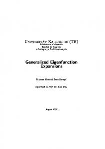
Figure 1: Numerically evaluated intensity correlation matrices Cαα′ defined in (44) for a complete graph with V = 16 vertices and B = 120 bonds. In the upper two panels the DFT scattering matrices have been used at each vertex. The lower two panels are for Neumann scattering matrices. For the right two panels time-reversal symmetry has been broken by adding a magnetic field. The directed bonds α = (b, d) have been ordered as ((1, −), (2, −), . . . , (B, −), (1, +), . . ., (B, +)). For the graphs in the orthogonal class on the left side there are four identical blocks as Cαα′ = Cα,α ˆ ′ = Cααˆ ′ = Cαˆ αˆ ′ . In the unitary case, note that the correlation matrix on the off-diagonal α = αˆ ′ remains strongly peaked for Neumann scattering matrices. However the four blocks are no longer the identical (this is not obvious from the picture). For DFT scattering matrices the strong off-diagonal peak almost disappears in the presence of a magnetic field.
13
In the limit B → ∞ (and constant degree q) one may replace the Circular Random Wave Model by the Gaussian Random Wave Model with the joint probability density ϕGU (a) ≡
B2B −2Bkak2 e . π2B
(48)
The predictions for the moments and the intensity correlation matrix in the Gaussian Random Wave Model read MGU,α,q =
q! (2B)q
and CGU,α,α′ =
1 + δαα′ (2B)2
(49)
which is equivalent to the leading order of the predictions (47) of the Circular Random Wave Model as B → ∞. If the eigenfunction statistics (37) of a family of quantum graphs in the unitary symmetry class are well reproduced by ϕCU (a) in (46) or by ϕGU (a) in (48), these formulae provide us with a universal Circular or Gaussian Random Wave Model, which gives access to all the statistical properties of the eigenfunctions. Notice that the exact calculation (41) asserts that (48) is the only possible Gaussian joint probability density function of the type (38), and hence, a non-universal Gaussian model cannot be realized on quantum graphs. Establishing the possible validity of the Gaussian Random Wave Model (48) would require the calculation of (37) for arbitrary products of amplitudes aβ . Note that the Gaussian Random Wave Model is consistent with the gauge principle, i.e. its prediction for any correlation function that is not explicitly gauge invariant vanishes identically. In what follows we will mainly focus on the explicitly gauge invariant autocorrelation functions (42). However in subsection 4.2 we will show that some low order correlation functions that are not explicitly gauge invariant indeed vanish on the level of the diagonal approximation. When time-reversal symmetry is conserved one has to take into account that the amplitudes of counter propagating waves on the same bond are complex conjugates, so that the wave function is real. We can thus only expect that a universal joint probability function is invariant under a 7→ ua where u is a unitary 2B × 2B matrix that respects reality of the wave function or, equivalently, that S 7→ u† S u conserves S T = S . Such unitary matrices have the block structure ! u∗++ u+− (50) u= ∗ u+− u++ in terms of the direction index d. Here u++ and u+− are two B × B matrices which are only constrained by unitarity of u. Unitary matrices with this block structure obey uT = u† = u−1 and are thus in fact orthogonal matrices with respect to T -transposition. The Circular Random Wave Model for the orthogonal class ! 1 2B−1(B − 1)! B ∗ 2 (51) δ (a+ − a− ) δ − ka+ k ϕCO (a) ≡ πB 2 is the unique model which respects a+ = a∗− , the normalization kak2 = 1 = 2ka+ k2 , and is invariant under the generalized orthogonal transformations (50). It gives the 14
predictions MCO,α,q CCO,α,α′
q!(B − 1)! = q 2 (B + q − 1)! 1 + δαα′ + δααˆ ′ = 4B(B + 1)
! q(q − 1) q! −2 1− = + O(B ) (2B)q 2B ! 1 1 + δαα′ + δααˆ ′ −2 1 − + O(B ) . = B (2B)2
(52)
The only difference in the leading order for large graphs is the term δααˆ ′ which ensures that the intensity correlation matrix is invariant under α 7→ α. ˆ Note that the deviations in the next order are twice as large in the orthogonal case. In the limit B → ∞ one may again replace the Circular Random Wave Model by a Gaussian Random Wave Model with the joint probability density ϕGO (a) ≡
BB B 2 δ (a+ − a∗− ) e−2Bka+ k πB
(53)
where only one half of the coefficients is taken from a Gaussian ensemble while the other half remains fixed by the symmetry constraints. The moments and the intensity correlation matrix in this Gaussian Random Wave Model are just the leading order terms from (52) MGO,α,q =
q! (2B)q
and CGO,α,α′ =
1 + δαα′ + δααˆ ′ . (2B)2
(54)
Note that the unitary and orthogonal universal Gaussian Random Wave Models (48) and (53) do not obey the normalization condition kak2 = 1. In fact one has E D E D kak2 = kak2 = 1. (55) GU
GO
only as an average property while the variances �� �� �2 � �2 � 1 1 = kak2 − 1 = kak2 − 1 and 2B B GU GO
(56)
are positive. Similarly, |aνα | cannot exceed one while the Gaussian Random Wave Models have a finite probability for this event. The Circular Random Wave Models take all these constraints into account correctly. There is another obstruction to all the Random Waves Models (46), (48), (51) and (53). The matching conditions at vertex i impose some correlation between the amplitudes supported on the neighboring bonds. This type of local and system-dependent correlations is ignored in the universal Random Wave Models. The most striking example consists in adding a Neumann vertex on some bond b of an ergodic graph. By doing so, the bond b is split into two new bonds b1 and b2 , which can be oriented such that (b1 , +) → (b2 , +). Then, the Neumann condition imposes |ab1 + |2 = |ab2 + |2 and |ab1 − |2 = |ab2 − |2 . These strong correlations contradict the predictions (47) and (52). Hence, a necessary condition for the universal Gaussian models (48) and (53) to be fulfilled in the limit of large graphs is that all the valencies tend to infinity. For a finite graph one should expect that none of these models reproduces the exact correlation functions. Indeed, any numerical evaluation of the wave function statistics 15
shows (amongst other things) an intensity fluctuation matrix that is far less uniform than the predictions from the Random Wave Models (see Figure 1). The deviations can only be expected to vanish as B → ∞ and if certain other conditions that we are going to derive are also satisfied.
3.3 Asymptotic Quantum Ergodicity Let G be a metric graph with B bonds. An observable on G is a family o n � V = Vb ∈ C 0 [0, Lb ] b ∈ NB
(57)
of B real functions Vb (x) defined on the bonds of G. The mean value V¯ of an observable V is defined by Z ⊕ B Z 2 2 X Lb V¯ ≡ Vb (x)dx. (58) V≡ trL G trL b=1 0 R⊕ Notice that trL 2 = G 1 is the volume of G. If an observable V is constant on each bond, one can simply write V = (Vb )b∈NB with Vb ∈ R. The mean value of such an observable reads PB b=1 Vb Lb ¯ (59) V= P B b=1 Lb
and is invariant under a global scaling of the bond lengths. Suppose now that S ∈ U(2B) is a scattering matrix on G. The quantum graph (G, S ) is said to be quantum ergodic if and only if there exists a subsequence i 7→ ν(i) of density 1 such that � Ψν(i) , VΨν(i) (60) lim � = V¯ i→∞ Ψν(i) , Ψν(i) LB ν for any observable V. In this definition, Ψν = b=1 ψb denotes an eigenfunction of H 2 of eigenvalue kν . By assumption, it is unique up to multiplication by complex numbers (or by real numbers for the orthogonal class). The left-hand side of (60) represents the mean value of the observable V in the eigenstate Ψν(i) . A straightforward calculation shows that (Ψν , VΨν )
=
B � X �Z |aνb+ |2 + |aνb− |2 b=1
+2ℜ
B X
ν aν∗ b− ab+
b=1
Z
0
Lb
Lb
Vb (x)dx 0
Vb (x)e2ikν
�
x−
Lb 2
�
dx
(61)
for the wave function Ψν with wave number kν > 0 and amplitudes aνb+ and aνb− as in ν (12). Since the observable V is assumed continuous on each bond, and since |aν∗ b− ab+ | ≤ −1 1, the second term in the right-hand side of (61) is O(kν ). In the high energy limit this second term gives no contribution to the left-hand side of (60). Moreover, the first term in the right-hand side of (61) remains unchanged if the observable V is replaced with
16
R Lb the observable W defined by Wb ≡ L−1 Vb (x)dx. These two remarks imply that, in b 0 the definition (60) of quantum ergodicity, it is sufficient to consider observables that are constant on each bond, and this will always be the case in what follows. If the equality (60) holds for any observable of vanishing mean V¯ = 0, then it also ¯ holds for any observable W. In order to see this, it is sufficient to observe that W − W has vanishing mean and to apply (60) to this new observable. Hence, without loss of generality, one can also restrict attention to observables V with V¯ = 0. If the identity (60) is satisfied for any subsequence of eigenfunctions, the quantum graph is said to be quantum unique ergodic. In [38], it is shown that many short closed cycles, like the triangle β1 → β2 → β3 → β1 for instance, support eigenfunctions with arbitrarily high energies. These eigenfunctions, called scars, break quantum unique ergodicity. While these scarred eigenfunctions were obtained explicitly for Neumann quantum graphs, quantum unique ergodicity should certainly not be expected to hold on general finite quantum graphs. Moreover, quantum ergodicity is generally not realized on a finite quantum graph as well. This notion has thus to be replaced with a weaker one which we call asymptotic quantum ergodicity. Let us consider an infinite sequence {(Gl , S l )}l∈N of quantum graphs with increasing number of bonds Bl < Bl+1 . We also suppose that the bonds of any Gl have bond lengths that satisfy Lb ∈ [Lmin , Lmax ]
where
0 < Lmin < Lmax < ∞
(62)
are independent of l. Such a sequence will be called increasing. We always assume that either all the graphs (Gl , S l ) are time-reversal invariant, or they all break this symmetry. The eigenfunctions of (Gl , S l ) are denoted by Ψνl , and similarly, all the quantities introduced above are indexed by l. Besides, a sequence {Vl }l∈N , where Vl is an observable on Gl , is said to be acceptable if and only if the two conditions liml→∞ V¯ l ≡ V¯ ∞ exists, 0 ≤ |Vl,b | ≤ Vmax
(63)
are fulfilled. Then, an increasing sequence {(Gl , S l )}l∈N of quantum graphs is said to be asymptotically quantum ergodic if and only if lim lim
l→∞ i→∞
� Ψlν(i) , Vl Ψν(i) l = V¯ ∞ ν(i) � Ψν(i) l , Ψl
(64)
for all acceptable sequences of observables {Vl }l∈N . The limit l → ∞ plays the role of the semiclassical limit for quantum graphs. For the sequences of graphs satisfying (64), the rate of convergence is also of particular interest. Therefore, we will treat a single finite quantum graph first, and come back to convergence and rate considerations afterwards. A calculation similar to (61) shows that, for an observable V on G constant on each bond, one has ! + * � sin(kν L) ν ν ν −1 (65) Ψν , VΨν = aν VL 1 + a = ha |VL|a i + O(kν ), kν L 17
where |aν i ∈ A is the vector of amplitudes defining Ψν through the construction (12). There is a slight abuse of notation in this expression. On the left-hand side, V = (Vb )b∈NB is an observable constant on each bond, whereas on the right-hand side V stands for the diagonal 2B × 2B matrix Vbd,b′ d′ ≡ δb,b′ δd,d′ Vb . Such a matrix is called observable on A and has mean value P2B PB tr(VL) β=1 Vβ Lβ b=1 Vb Lb V¯ ≡ . (66) = P = P2B B trL b=1 Lb β=1 Lβ
This expression coincides with the mean value (59) of V seen as an observable on G constant on each bond. From (60), (65) and (66), we deduce that a quantum graph is quantum ergodic if and only if there exists a subsequence i 7→ ν(i) of density 1 such that hVLiν(i) haν(i) |VL|aν(i) i ¯ ≡ lim =V i→∞ haν(i) |L|aν(i) i i→∞ hLiν(i) lim
(67)
for any observable V on A. As above, one can restrict attention to observables V such that V¯ = 0 without loss of generality. A standard theorem of ergodic theory, proven for example in [45], states that the quantum ergodicity property (67) is equivalent to the vanishing of FV ≡ lim
K→∞
1 X hVLi2ν N(K) k ≤K hLi2ν
(68)
ν
for all observables V on A with V¯ = 0. Moreover, since the bond lengths are bounded by Lmin and Lmax by assumption (62), this property is also equivalent to the vanishing of the fluctuations !2 2B � � 2B X VL β VL β′ Cββ′ (69) FV ≡ trL β,β′ =1 for all observables V on A with V¯ = 0, where the intensity correlation matrix Cββ′ in the right-hand side is defined in (44). In the case of an increasing sequence of graphs {(Gl , S l )}l∈N , asymptotic quantum ergodicity is obeyed if and only if the sequence {Fl,Vl }l∈N whose terms are defined as in (68), or equivalently the sequence {Fl,Vl }l∈N whose terms are defined as in (69), converges to zero as l → ∞ for all acceptable sequences of observables {Vl }l∈N . The rate of convergence is then called the rate of quantum ergodicity. The Gaussian Random Wave Models (48) and (53) predict the fluctuations FV = V¯ 2 + κ
tr(VL)2 , (tr L)2
(70)
as can easily be shown from the Gaussian predictions for the intensity correlation matrix (49) and (54). The parameter κ was defined in (28). The term proportional to κ describes the deviation from quantum ergodicity. For any admissible observable and bond lengths bounded by (62) the deviation predicted by the Gaussian Random Wave 18
Models is O(B−1 ). Hence the Gaussian Random Wave Models predict that any increasing sequence of quantum graphs is asymptotically quantum ergodic and that the rate of convergence is larger by a factor of two if time-reversal symmetry is conserved. Note, that quantum ergodicity holds on average, in the sense that 1 X hVLiν AV ≡ lim = V¯ (71) K→∞ N(K) hLiν k ≤K ν
for all observables V. This is known as the local Weyl law. It is easily checked to hold for any quantum graph . Indeed, by the definition (42), AV can also be written 2B
AV =
E D 2B X (VL)β |aβ |2 . trL β=1
(72)
D E Then, the identity (41) shows that |aβ |2 = (2B)−1, and the definition (66) of V¯ concludes the proof of the claim. The restriction to incommensurable bond lengths is not necessary for the local Weyl law, indeed we will show in the following subsection that (41) is true for any choice of bond lengths.
3.4 Green Matrices and Trace Formulae For (G, S ) a quantum graph, and for ǫ > 0, one defines a sub-unitary quantum map Uǫ (k) by Uǫ (k) = T (k)S ǫ T (k), with S ǫ ≡ e−ǫ S , (73) and where T (k) is the propagation matrix of G given in (16). The retarded Green matrix (resolvent) G(k) is the matrix-valued function on R+ defined by 2B � �−1 X |n, kihn, k| . G(k) ≡ 1 − Uǫ (k) = 1 − ei(φn (k)+iǫ) n=1
(74)
It has poles in the lower complex half-plane at φn (k) = 2πp − iǫ for any p ∈ Z. The advanced Green matrix G† (k) is the hermitian conjugate of G(k), that is 2B � �−1 X G† (k) = 1 − Uǫ† (k) = n=1
|n, kihn, k| . 1 − e−i(φn (k)−iǫ)
(75)
It has poles in the upper complex half-plane at φn (k) = 2πp + iǫ for any p ∈ Z. Making use of formula (25), it is not difficult to check that, for any integer q ≥ 2, and for any permutation σ ∈ S q , the statistical quantities defined in (37) with p = q read q−1
E (2ǫ)q−1 D Y G(k)βσ( j) β′j · G† (k)βσ(0) β′0 , k ǫ→0 2B j=1
ha∗β0 . . . a∗βq−1 aβ′0 . . . aβ′q−1 i = lim
where, in the right-hand side, the average over k is defined by the formula Z K
� 1 f (k) k ≡ lim f (k)dk K→∞ K 0 19
(76)
(77)
which is meaningful for any function f integrable on every compact interval [0, K]. The formula (76) relies on the non-degeneracy of the spectrum, which generically follows from the incommensurability of the bond lengths. However, it still holds if the subsequence of levels kν that are degenerate is of density zero. There are other versions of the equality (76) where the right-hand side involve nr ∈ N elements of G(k) and na ∈ N elements of G† (k) with nr + na = q. A formula similar to (76) is used in [20] to study the statistical properties of the eigenfunctions in disordered systems. For the derivation of exact expressions the choice of the permutation σ ∈ S q in (76) is mainly a matter of computational ease (and sometimes taste). Throughout the remainder of this subsection we will show how the different choices lead to different exact expressions. The Green matrices G(k) and G† (k) can be viewed as the results of summing geometrical series in Uǫ (k) and Uǫ† (k). This gives rise to interpretations of their components as sums of walks on the quantum graph (G, S ). An oriented walk ~β is a list (β0 , β1 , . . . , βn ) of consecutive directed bonds on the graph. Its topological length |~β| is the number of vertices traversed, that is |~β| = n. The set of all oriented walks having topological length n is written Wn . The metric length of ~β is l(~β) ≡
n−1 Lβ0 X Lβ + Lβi + n . 2 2 i=1
(78)
The origin and terminus of ~β are respectively o~β ≡ β0 and t~β ≡ βn . The set of walks in Wn having origin β and terminus β′ is written Wn (β, β′ ), and ∪n∈N0 Wn (β, β′ ) ≡ W(β, β′ ). We also define the stability amplitude A~β ≡
n−1 Y
S βi+1 βi .
(79)
i=0
With these definitions, it is easy to see that X ~ ~ G(k)ββ′ = e−ǫ|β| eikl(β) A~β
(80)
~β∈W(β′ ,β)
and G† (k)ββ′ =
X
~
~
e−ǫ|β| e−ikl(β) A~β ∗ .
(81)
~β∈W(β,β′ )
Together with (76), these formulae enable one to express the autocorrelation functions C[α] in (42) as sums over oriented walks. The different choices for the order of the left indices β in (76) lead to different equivalent expressions for the autocorrelation functions C[α] in terms of oriented walks. In general, showing the equivalence between these trace formulae at the level of oriented walks turns out to be a very difficult problem. In this subsection, these non-trivial equivalences are illustrated by two alternative proofs of the local Weyl law (71). In the case of the intensity correlation matrix Cββ′ , two permutations σ ∈ S 2 of the
20
β
β S
Cββ ′ =
β~
P
=
β~ ′
β~ ∈ W (β, β) β~ ′ ∈ W (β ′, β ′) ~ = l(β~ ′) l(β)
S
P
β~ ′ β~ S
S†
β~ ∈ W (β, β ′) β~ ′ ∈ W (β ′, β) ~ = l(β~ ′) l(β)
†
β′
β′
Figure 2: The two equivalent formulae (83) and (85) for the autocorrelation function Cββ′ . The underlying graph has not been represented for sake of clarity. The trace formulae (88) and (89) are obtained from the ones represented here by adding the contributions where S and S † are swapped and by dividing by two.
left indices in (76) can be chosen. The identity permutation σ = id leads to E ǫ D G(k)ββG† (k)β′ β′ Cββ′ = lim k ǫ→0 B X ǫ X −ǫ(|~β|+|~β′ |) = lim e δl(~β),l(~β′ ) A~β Aβ~′ ∗ ǫ→0 B ′ ′ ′
(82) (83)
~β∈W(β,β) ~β ∈W(β ,β )
while choosing the transposition σ = (1 2) leads to Cββ′
= =
E ǫ D G(k)β′ βG† (k)ββ′ k ǫ→0 B X ǫ X ~ ~′ lim e−ǫ(|β|+|β |) δl(~β),l(~β′ ) A~β A~β′ ∗ . ǫ→0 B ′ ′ ′ lim
(84) (85)
~β∈W(β,β ) ~β ∈W(β,β )
In both cases, the Kronecker symbols originate from the average over k. These orbit expressions can also be recovered by means of the Poisson summation formula. If δǫ (x) denotes the Lorentzian of width ǫ centered at the origin, this formula leads to Gǫ (k)
≡ =
2B X n=1
|n, kihn, k|
∞ X p=0
δǫ φn (k) − 2πp
∞
�
� 1 X 1 U(k)q + U † (k)q e−ǫq 1+ 2π 2π q=1
(86)
(87)
The trace formula (83), or more exactly its symmetrization obtained by replacing A~β A~β′ ∗ with 12 (A~β A~β′ ∗ + A~β ∗ A~β′ ), follows from (87) and the identity Cββ′ =
E 2π2 ǫ D Gǫ (k)ββ Gǫ (k)β′ β′ k B 21
(88)
This identity is a consequence of the fact that, in terms of distributions, the product 2πǫδǫ (x)δǫ (y) tends to zero if x , y and to δ(x) if x = y. Similarly, the symmetric version of (85) follows from (87) and Cββ′ =
E 2π2 ǫ D Gǫ (k)β′ β Gǫ (k)ββ′ . k B
(89)
The main advantage of the expressions (88) and (89), involving Gǫ (k), over their analogues (82) and (84), which involve G(k), is that the matrix Gǫ (k) is real, whereas G(k) and G† (k) have non-vanishing imaginary D parts E and must always appear together in (76). In particular, the first moment Mβ,1 = |aβ |2 can be written D E π lim Gǫ (k)ββ k , ǫ→0 B
Mβ,1 =
(90)
which involves a single closed oriented walk, while, in terms of matrices G(k), an additional directed bond β′ Dmust first Ebe introduced in order for Mβ,1 to be written as P2B P 2 2 and the representations (83) or (85) to be used. the sum 2B β′ =1 |aβ | |aβ′ | β′ =1 Cββ′ = From (87) and (90), one finds directly that Mβ,1 =
1 , 2B
(91)
which, together with (72), provides a second proof of the local Weyl law. Let us now use the trace formula (85) and perform the sum over the directed bond β′ . It is easy to show by induction over n and m that the unitarity of the scattering matrix S implies 2B X
β′ =1
X
X
δl(~β),l(~β′ ) A~β A~β′ ∗ = δn,m
(92)
∞ 1 ǫ X −ǫ(n+m) e δn,m = , B n,m=0 2B
(93)
~β∈Wn (β,β′ ) ~β′ ∈Wm (β,β′ )
for all n, m ∈ N0 . With (85), this gives Mβ,1 =
2B X
β′ =1
Cββ′ = lim
ǫ→0
which, together with (72), yields a third proof of the local Weyl law. The choice for the permutation σ ∈ S q in (76) leads, in the case q = 2, to the equivalent expressions (83) and (85) for Cββ′ in terms of oriented walks that are illustrated in Figure 2. Similar pictures could also be drawn for C[β0 ,...βq−1 ] when q > 2 . Indeed, the right-hand side of (76) with β′j = β j for all 0 ≤ j ≤ q − 1 and with a fixed permutation σ ∈ S q can be expressed as a sum over q oriented walks ~β1 , . . . , ~βq , where each ~β j leads from the directed bond β j to the directed bond βσ( j) . The walk ~βq is followed with S ǫ† , whereas the q − 1 other walks are followed with S ǫ , and its metric length must equal the sum of the metric lengths of the q − 1 other walks. Therefore, (76) yields q · q! different ways of expressing the autocorrelation function C[β] of degree q in terms of oriented walks. Here, the first factor q accounts for the q possible choices for the walk followed with S ǫ† . 22
3.5 Long Diagonal Orbits An expression for the fluctuations FV in (69) can be obtained by retaining only a subset of the whole set of pairs of oriented walks (~β, ~β′ ) entering (83). For this purpose, it is convenient to come back to the expression (88) of Cββ′ in terms of Gǫ (k) and write the fluctuations of an observable V with V¯ = 0 as FV =
8Bπ2ǫ D �� E tr Gǫ (k)VL 2 . 2 k (trL)
(94)
The right-hand side can be written in terms of periodic orbits rather than closed oriented walks as in (83). A periodic orbit is an equivalence class of closed oriented walks whose sequences of directed bonds differ from each other by cyclic permutations. For a periodic orbit p, the notions of reverse p, ˆ topological length |p|, metric length l p and stability amplitude A p are inherited from the oriented walks terminology, and the repetition number r p is the number of times p retraces itself. With this notation, one gets from (87) 1 X −ǫ|p| (VL) p ikl p e Ap, (95) e tr (Gǫ VL) = ℜ π rp p where the sum is over all the periodic orbits on the graph and (VL) p stands for the number obtained by accumulating the values (VL)β of VL along p. The square of the last formula admits the spectral average D� �� E 1 X (VL) p (VL)q ℜ(A p A∗q )e−ǫ(|p|+|q|) . tr Gǫ VL 2 = 2 k r p rq 2π p,q:l =l p
(96)
q
The diagonal approximation, which consists in only keeping the pairs q = p and q = pˆ in the time-reversal invariant case, yields D�
�2 � �� Ediag κ X (VL) p = 2 tr Gǫ VL 2 |A p |2 e−2ǫ|p| , k 2π p,q:l =l r2p p
(97)
q
where κ is the parameter as in (70) indicating whether time-reversal invariance is broken or conserved. We have neglected some corrections in the diagonal approximation which are due to repetitions and self-retracing orbits. These can be shown not to contribute in the present context. The formula (97) is then approximated further. The orbits for which r p > 1 are rare, so that we only keep the primitive orbits, namely those with r p = 1. We also take the long orbits approximation [18], which amounts to approximating � � � tr(VL)2 � (VL) p 2 ≈ (VL)2 p ≈ |p| . (98) 2B Besides, the stability amplitude is known to behave like [25] |A p |2 ∼ e−α|p| ,
23
(99)
where α is the topological entropy. This parameter also characterizes the number |p|−1 eα|p| of periodic orbits having topological length |p|. With all these approximations, (97) reduces to the integral Z ∞ α|p| D� κ ��2 Ediag tr(VL)2 −α|p| −2ǫ|p| e d|p| ≈ 2 tr Gǫ VL · |p| ·e ·e . (100) k |p| 2B 2π 0 Hence
tr(VL)2 . (101) (trL)2 This formula, obtained from the long diagonal orbits, coincides with the prediction (70) of the Gaussian Random Wave Models (48) and (53). It predicts asymptotic quantum ergodicity for any increasing sequence of quantum graphs and a universal rate of convergence B−1 , as in [18]. diag
FV
≈κ
4 Generating Functions 4.1 Definition and Principles The Green matrices introduced in the subsection 3.4 can be obtained as the derivatives of certain determinants. It is convenient first to introduce a Grassmann algebra Λ, which can be decomposed as the direct sum of its commuting sub-algebra ΛB , called bosonic, and a set ΛF of elements anticommuting with each other, called fermionic. Then, the amplitude space A can be graded to get A ⊕ A, and the Grassmann envelope (A ⊕ A)(Λ) defined as in [5] can be built. This set reads ! 2B X VB β β (A ⊕ A)(Λ) ≡ ; VB/F = V= , (102) VB/F |eβ i, VB/F ∈ ΛB/F V F β=1
where the elements |eβ i refer to the elements in (11) of the natural basis of A. The elements of (A ⊕ A)(Λ) are called supervectors. The set of endomorphisms on (102), once written in the natural basis of A, form a set of supermatrices written L(A|A). For q ≥ 2 an integer, let us introduce complex numbers j1 , . . . , jq−1 and j0 , respectively referred to as retarded and advanced sources, and let us also consider q directed bonds α1 , . . . αq−1 and α0 . The corresponding retarded and advanced source supermatrices are defined by Jr ( j r ) ≡
Ja ( ja ) ≡
1 + E B ⊗ j r E(r) ,
(103)
(a)
1 + E B ⊗ ja E ,
where E B is the projector onto the bosonic sector of (A ⊕ A)(Λ), E α0 ,α0 j0 ! ! j E α1 ,α1 (a) 1 E ja ≡ j≡ ≡ . , E ≡ .. (r) . E jr . αq−1. ,αq−1 E jq−1 24
(104)
,
(105)
′
and, for any two directed bonds α, α′ ∈ N2B , E α,α stands for the 2B × 2B matrix whose ′ components are (E α,α )ββ′ ≡ δα,β δα′ ,β′ in the natural basis of A. The number q − 1 of retarded sources corresponds to the number of matrices E α j ,α j contained in E(r) , so that the product in (103) makes sense. In (103), (104) and in what follows, some unit matrices or supermatrices are not explicitly written in order to keep the notation as simple as possible. For example, the symbols 1 in (103) and (104) must be read 1BF ⊗1A , where 1BF is the unit supermatrix in Bose-Fermi space and 1A is the 2B×2B unit matrix in amplitude space A. Let q ≥ 2 and let [α] ≡ [α0 , α1 , . . . , αq−1 ] be a list of q directed bonds. The corresponding generating function is defined by D � �� �E (106) ξ[α] ( j) ≡ sdet−1 1 − Jr ( j r ) · Uǫ (k) 1 − Ja ( ja ) · Uǫ† (k) , k
where Jr ( j r ) and Ja ( ja ) are defined from j ≡ ( ja , j r )T = ( j0 , j1 , . . . , jq−1 )T and from the directed bonds in [α] as in (103) and (104). Notice that this function is well defined in a neighborhood of the origin, and that it also reads D � ��� ��E (107) ξ[α] ( j) = det−1 1 − j r E(r) G(k) − 1 1 − ja E (a) G† (k) − 1 k
in terms of Green matrices. It is convenient at this point to give a general rule governing derivatives of determinants of the form (107). An important quantity is the ρ factor ρα (σ) ≡ αnumber of cycles in σ
(108)
defined for any α ∈ R and any permutation σ ∈ S s of s ∈ N elements. This factor can be seen as a generalization of the signature (−1)σ of σ ∈ S s since the identity (−1)σ = (−1) sρ−1 (σ) holds. Now, if A = (A(1) , . . . , A(s) )T is a vector containing s ∈ N square matrices A(i) of size n ∈ N and if j ∈ C s , we have the equality s X n X Y ∂s ρα (σ) A(i) det (1 − j A)−α = xi ,xσ(i) . ∂ j1 . . . ∂ j s j=0 σ∈S i=1 x =1 s
(109)
i
This result can be proved by induction over s. The right-hand side has a natural diagrammatic representation where each i ∈ N s is a point and where an arrow is drawn from i to j whenever σ(i) = j. The sum in (109) is then the sum over all such diagrams in which each point i ∈ N s has exactly one outgoing and �one incoming arrow. The � p value of each diagram is a product of traces of the type tr A(i) Aσ(i) · · · Aσ (i) , with p being the smallest number in N0 such that σ p+1 (i) = i, weighted by its ρ factor, which can be deduced from the number of connected sub-diagrams. Let q ≥ 2 and let [α] ≡ [α0 , α1 , . . . , αq−1 ] be a list of q directed bonds. The rule (109) can be applied to the expression (107) for the generating function, and, making use of (76), one easily gets (2ǫ)q−1 δξ[α] , ǫ→0 2B(q − 1)!
C[α] = lim
25
(110)
where C[α] is the autocorrelation function defined in (42), and q−1 Y ∂ ξ[α] . δξ[α] ≡ ∂ js s=0
(111)
j=0
The denominator (q−1)! in (110) comes from the number of diagrams arising when the rule (109) is applied to the q − 1 retarded derivatives on ξ[α] ( j). By (76), these diagrams all yield the same contribution. It is not difficult to check that the generating functions have the following property. For all ja and j r = ( j1 , . . . , jq−1 ) in a sufficiently small neighborhood of the origin, ξ[α] ( ja , 0) = ξ[α] (0, j r ) = 1.
(112)
σ For σ ∈ S q and [α] ≡ [α0 , α1 , . . . , αq−1 ], one can introduce a function ξ[α] ( j) by the α j ,ασ( j) α j ,α j formula (106) using the matrices E in place of E in the source supermatrices, σ σ and (110) then serves as a definition for C[α] . The function ξ[α] ( j) also satisfies the σ property (112), and the identities (76) and (109) ensure that C[α] = C[α] for any σ ∈ S q . σ In what follows, the arbitrary choice for σ ∈ S q in ξ[α] ( j) will be called the choice of convention. These different but equivalent expressions must not be confused with the equivalent sums over orientated walks which are the object of Subsection 3.4. Any convention σ ∈ S q for the generating function involves (q − 1)! equivalent sums over orientated walks. However, in the case q = 2, the permutations σ = id and σ = (0 1), which are referred to as parallel and crossed conventions in the sequel, do correspond to the sums (83) and (85) respectively. We started this chapter with the convention to choose σ ∈ S q to be the identity and we will use this convention in most of the following calculations. This convention is not only singled out by simplicity; it results in a generating function (106) that is explicitly gauge invariant while in other choices the gauge invariance is only restored in the limit (110). It also reduces the complexity of some calculations because the matrices Jr ( jr ) and Ja ( ja ) for the source terms (103) are diagonal matrices. While each convention yields a different but exactly equivalent expression approximation schemes may break the exact identity. This is not worrying as long as the difference is in sub-leading order. For time-reversal invariant graphs the generating function (106) is usually not explicitly invariant when one replaces any directed bond by its reversed partner for q ≥ 3. The invariance is only revealed once the derivative in (110) is taken (the limit ǫ → 0 is not required).
4.2 Diagonal Approximation Before working further on the generating function (106) with the supersymmetry method we introduce in this subsection similar generating functions and develop a corresponding trace formula. The diagonal approximation to this new type of generating functions turns out to behave very differently from the oriented walk representations previously discussed in the subsections 3.4 and 3.5. The definition (106) of the generating functions, and the fundamental formula (110) can easily be generalized to any correlation function (37) with p = q. Moreover, these 26
correlation functions can also be written in terms of logarithmic derivatives with some analogy to (110). We will focus on the case p = q = 2 for which the general correlation function can be written as E D ǫ a∗α1 aα′1 ∗ aα2 aα′2 = lim δΞ[α1 ,α′1 ;α2 ,α′2 ] , (113) ǫ→0 B where Ξ[α1 ,α′1 ;α2 ,α′2 ] ( ja , jr ) ≡ =
D
� � � �E log det 1 − J˜r ( jr )Uǫ (k) log det 1 − J˜a ( ja )Uǫ† (k) k D � � � �∗ E ,(114) log det 1 − J˜r ( jr )Uǫ (k) log det 1 − J˜a ( ja )T Uǫ (k) k
the source terms are given by ′ ′ J˜r ( jr ) = 1 + jr E α1 ,α2 and J˜a ( ja ) = 1 + ja E α1 ,α2 , (115) 2 . The intensity correlation matrix can be obtained in two and δΞ ≡ ∂ j∂r ∂ ja Ξ( ja , jr ) ja = jr =0 different ways
Cαα′ = limǫ→0 Bǫ δΞ[α,α′ ;α,α′ ]
(116)
limǫ→0 Bǫ δΞ[α,α′ ;α′ ,α]
(117)
=
referred as parallel and crossed conventions, respectively. In the orthogonal class one has a third representation ǫ (118) Cαα′ = lim δΞ[α,α;α ˆ ′ ,αˆ ′ ] ǫ→0 B called time-reversed crossed convention. The formula log det = tr log enables us to write the new generating function (114) in terms of generalized periodic orbits on the graph. Indeed, expanding the logarithms and performing the spectral average yields the trace formula Ξ[α1 ,α′1 ;α2 ,α′2 ] ( ja , jr ) =
X
X
p∈Pα1 α2 p′ ∈Pα′ α′
2 1
∞ X � �ρ′ 1 Ar,p ( jr )ρ Aa,p′ ( ja )∗ δρl p ,ρ′ l p′ ′ ρρ ρ,ρ′ =0
(119)
where the retarded and advanced modified stability amplitudes Ar,p ( jr ) and Aa,p ( ja ) of the generalized periodic orbit p = β1 β2 . . . β|p| are defined by Ar,p ( jr ) ≡
|p| Y � i=1
� J˜r ( jr )S ǫ βi+1 βi
and
Aa,p ( ja ) ≡
|p| Y � i=1
� J˜a ( ja )T S ǫ βi+1 βi .
(120)
The periodic orbits p and p′ in (119) are all primitive but can be of a slightly more general type than the primitive periodic orbits considered in Subsection 3.5. Indeed, the retarded source term in (115) introduces the possibility to jump α2 y α1 , and similarly the advanced source term introduces the possibility to jump α′1 y α′2 . The set Pα1 α2 in (119) then contains all the primitive periodic orbits that are compatible with the topology of the graph with an additional bridge α2 y α1 at the center of these 27
directed bonds. Note that the two sets Pα1 α2 and Pα′2 α′1 of generalized periodic orbits need not be identical. In the parallel convention for Cαα′ , the source terms are diagonal matrices, and Pαα ≡ P reduces to the set of standard primitive periodic orbits, which only respect the topology of the graph. The length of a generalized periodic orbit is just the sum of all bond lengths along the periodic orbit, where every jump α2 y α1 contributes 12 (Lα1 + Lα2 ). In the trace formula (119), only pairs of primitive orbits contribute such that a repetition of one orbit has the same length as a repetition of the other. The diagonal approximation to the trace formula (119) reduces the sum over pairs of primitive orbits to either equal orbits p′ = p, or time-reversed orbits p′ = p. ˆ In both cases, the factor δρl p ,ρ′ l p′ enforces ρ = ρ′ . Note that p has to be a periodic orbit in the intersection p ∈ Pα1 α2 ∩ Pα′2 α′1 to contribute to the diagonal approximation. The remaining sum over periodic orbits can be resummed diag
diag,D
Ξ[α1 ,α′ ;α2 ,α′ ] ( ja , jr ) = Ξ[α1 ,α′ ;α2 ,α′ ] ( ja , jr ) 1 2 1 �2 � = − log det 1 − M D ( ja , jr )
diag,C
+ Ξ[α1 ,α′ ;α2 ,α′ ] ( ja , jr ) 1 � 2 � − log det 1 − MC ( ja , jr )
+C +C (121)
where M D ( ja , jr ) and MC ( ja , jr ) are modifications of the classical map (32). They describe diffuson and cooperon propagations, which originate from pairs of periodic orbits with p′ = p and p′ = p, ˆ and are given by X M D ( ja , jr )β1 β2 ≡ Jr ( jr )β1 β′ Ja ( ja )β′ β1 |S ǫ, β′ β2 |2 β′
�
� = 1 + jr δβ1 α1 δα1 α2 + ja δβ1 α′2 δα′1 α′2 |S ǫ, β1 β2 |2 + C
M ( ja , jr )β1 β2
jr ja δβ1 α1 δα1 α′2 δα′1 α2 |S ǫ, α2 β2 |2 X � �∗ ≡ Jr ( jr )β1 β′ Ja ( ja )Tβ′ β1 S ǫ, β′ β2 S ǫ,T β′ β2
(122)
β′
� �∗ � = 1 + jr δβ1 α1 δα1 α2 + ja δβ1 αˆ ′1 δα′1 α′2 S ǫ, β1 β2 S ǫ, βˆ 2 βˆ 1 + �∗ � jr ja δβ1 α1 δα1 αˆ ′1 δα2 αˆ ′2 S ǫ, α2 β2 S ǫ, βˆ 2 αˆ 2 . �
(123)
The term C in (121) contains corrections for repetitions and self-retracing orbits (p = p) ˆ which can be shown not to contribute to our final result and will be omitted henceforth. Recall that the classical map is defined by Mβ1 β2 = |S β1 β2 |2 , so that M D (0, 0) = Mǫ ≡ −2ǫ e M. For time-reversal invariant systems, the products of scattering matrices in (123) reduces to S ǫ, β1 β2 (S ǫ, βˆ 2 βˆ 1 )∗ = |S ǫ, β1 β2 |2 = Mǫ,β1 β2 , so that limǫ→0 MC (0, 0) = M. If time reversal symmetry is broken MC (0, 0) does not reduce to M and it does not describe a Markof process on the graph. We will see that the cooperon term only contributes to the diagonal approximation formula if time-reversal symmetry holds.
28
The derivatives with respect to jr and ja can now be taken and yield " ! !# 1 ∂2 M D 1 ∂M D 1 ∂M D diag,D δΞ[α1 ,α′ ;α2 ,α′ ] = tr + tr 1 2 1 − Mǫ ∂ j+ ∂ j− 1 − Mǫ ∂ j+ 1 − Mǫ ∂ j− ja = jr =0 ! Mǫ + =δα1 α′2 δα′1 α2 1 − Mǫ α2 α1 ! ! Mǫ Mǫ δα1 α2 δα′1 α′2 (124) 1 − Mǫ α1 α′ 1 − Mǫ α′ α1 1
1
for the diffuson generating function, and diag,C δΞ[α1 ,α′ ;α2 ,α′ ] 1 2
=δ
α1 αˆ ′1
δ
α2 αˆ ′2
δα1 α2 δα′1 α′2
MC (0, 0) 1 − MC (0, 0) MC (0, 0) 1 − MC (0, 0)
! !
+ α2 α1
α1 αˆ ′1
MC (0, 0) 1 − MC (0, 0)
!
(125) α′1 αˆ 1
for the cooperon generating function. For broken time-reversal invariance the classical cooperon map MC (0, 0) has no unit eigenvalues in the limit ǫ → 0, and hence, (125) identically vanishes in that limit. By contrast, in time-reversal invariant systems MC (0, 0) = Mǫ and the cooperon generating function does contribute. Finally, only terms in (124) and (125) that are singular as ǫ → 0 contribute to the correlation function (113). In order to isolate these terms, one makes use of the decomposition (35) of classical orbits as the sum of a uniform component |1ih1| and a massive part R. This yields � κ(1 − 2ǫ) 1 � ǫ diag δΞ[α1 ,α′ ;α2 ,α′ ] = δα1 α2 δα′1 α′2 + δα1 α′2 δα′1 α2 + (κ − 1)δα1 αˆ ′1 δα2 αˆ ′2 + 3 2 1 2 B 16B ǫ 4B i� i h �h 1 + 2 δα1 α2 δα′1 α′2 Rα1 α′1 + Rα′1 α1 + (κ − 1) Rα1 αˆ ′1 + Rαˆ ′1 α1 + O(ǫ) 4B (126) After dropping terms that are O(ǫ), (126) may be expected to provide an approximation to the generating function (113). However, its first term diverges like ǫ −1 as ǫ → 0. At first sight, this seems to make periodic-orbit analysis using the trace formula (119) for the generating function much less useful than the previous trace formulae from Section 3.4 which behave nicely in the diagonal approximation. On the other hand, the same divergence also occurs in the analysis of spectral correlations, which become singular in the diagonal approximation at small energy differences. Indeed, one may obtain the corresponding trace formula for the spectral two point correlation function on a graph R2 (s) by replacing the source terms J˜a ( ja ) and J˜r ( jr ) appropriately. In this context, a supersymmetry method developed in [22, 23], which will be adapted to our purposes in what follows, cures the divergence. One may also try to add off-diagonal terms in the trace formula in a systematic way but we will not pursue this here. Note that the Kronecker symbols in the expression (126) force the correlation function ha∗α1 a∗α′ aα2 aα′2 i to vanish for all combinations that are not invariant under all local 1
29
gauge transformations allowed by the unitary or orthogonal symmetry class. The nonvanishing combinations are then equivalent to the three different conventions (116), (117) and (118) for expressing the intensity correlation matrix. These three conventions lead however to different formulae. κ For any of the three conventions (116), (117) and (118), if one replaces ǫ 7→ 4B , the first line in (126) reproduces the prediction of the Gaussian Random Wave Model up to corrections that are O(B−3 ). The second line in (126) then gives a correction in terms of system dependent massive modes. This massive correction turns out to be different for the three conventions of expressing Cαα′ . In the orthogonal class only the parallel convention (116) provides an approximated intensity correlation matrix that respects the identity Cαα′ = Cααˆ ′ satisfied by the exact intensity correlation matrix. By contrast, if either the crossed convention (117) or the time-reversed crossed convention (118) is used, the massive terms in the approximated intensity correlation matrix explicitly violate this symmetry. The origin of this discrepancy is that, with the parallel convention (116), each of the two logarithms in the generating function Ξ[α,α′ ;α,α′ ] ( ja , jr ) is invariant under time inversion, while in the crossed and time-reversed crossed conventions the symmetry is only restored after taking the derivatives and performing the limit ǫ → 0. The observations above concerning time-reversal symmetry makes the parallel convention (116) a privileged choice when it comes to the diagonal approximation. This convention yields ! 1 κ(1 − 2ǫ) diag,k + δαα′ + (κ − 1)δααˆ ′ + Rαα′ + Rα′ α + (κ − 1) (Rααˆ ′ + Rαˆ ′ α ) . Cαα′ = 4Bǫ 4B2 (127) The three first terms are universal, and are equal to the prediction of the Gaussian Ranκ (which we cannot justify at dom Wave Model if ǫ is chosen finite and set equal to 4B this stage). The remaining three terms involve the matrix R and they describe massive corrections to the universal result. In fact, these massive contributions may dominate the correlation functions and, as a consequence, the rate of convergence for quantum ergodicity, or they may destroy quantum ergodicity altogether. This point will be discussed further in Section 7.
4.3 Nonlinear Supersymmetric σ Model The generating functions in (106) depend strongly on whether time-reversal symmetry is broken or conserved. Time inversion acts on supervectors ψ in the Grassmann envelope (X ⊕ X)(Λ), defined from X = A ⊗ Cn for some n ∈ N0 as in (102), and on supermatrices A ∈ L(X|X) as T ψ = σd1 ψ∗
and
AT = σd1 AT σd1 .
(128)
In (128), σd1 is the first Pauli matrix acting on the direction space Ad , ψ∗ denotes the vector obtained from ψ by taking the complex conjugates of each component, and AT is the transpose of A defined as in [19] by the condition (Aψ1 )T ψ2 = ψT1 AT ψ2 for all ψ1 , ψ2 in (X ⊕ X)(Λ). Here and henceforth, ψT stands for the row vector obtained from 30
the column vector ψ ∈ (X ⊕ X)(Λ) by usual transposition. One can now introduce a 2-dimensional C-linear space T R, the time-reversal space, and the mapping ! ! 1 1 ψ ψ ψ 7→ Ψ ≡ √ = √ , (129) d ∗ 2 T ψ TR 2 σ1 ψ T R from (X ⊕ X)(Λ) to (X ⊗ T R ⊕ X ⊗ T R)(Λ) called time-reversal doubling. We work with the convention χ∗∗ = −χ for all χ ∈ ΛF as in [19], and hence, the Hermitian conjugate of Ψ in (129) reads � � ¯ = ψ† , ψT σd σBF , Ψ (130) 1 3
where ψ† = ψ∗T is the Hermitian conjugate of ψ, and σ3BF stands for the third Pauli matrix acting on the Bose-Fermi space. Similarly, the time-reversal doubling of a supermatrix A ∈ L(X|X) is defined by ! ! A 0 A 0 , (131) A 7→ A ≡ = 0 AT T R 0 σd1 AT σd1 T R
and is an element of L(X ⊗ T R|X ⊗ T R). In (129), (131) and in what follows, an index T R added to a supermatrix means that this supermatrix is explicitly written in the T R space, and the same notational trick is used for any other space. The components in time-reversal space will be indexed by t ∈ {↑, ↓}. The definitions above call for a notion of generalized transposition Aτ of A ∈ L(X ⊗ T R|X ⊗ T R), which is defined as in [23] by ! 0 σ3BF τ T −1 d A ≡ τA τ , where τ ≡ σ1 . (132) 1BF 0 TR ¯ 1 AΨ2 = Ψ ¯ 2 Aτ Ψ1 holds for any couple of This definition implies that the equality Ψ supervectors Ψ1 , Ψ2 ∈ (X ⊗ T R ⊕ X ⊗ T R)(Λ) and for any supermatrix A ∈ L(X ⊗ T R|X ⊗ T R). It follows that (Aτ )τ = A and (AB)τ = Bτ Aτ for any such supermatrices. Moreover, using the property (AT )T = σ3BF Aσ3BF of the transposition in L(X|X), it is easy to check that a supermatrix A obtained from some A ∈ L(X|X) by time-reversal doubling (131) is invariant under generalized transposition. Now, the generating functions can be written D �� �E 1� ξ[α] ( j) = sdet−1 Jr Ja sdet− 2 Jr−1 − Uǫ (k) Ja−1 − Uǫ† (k) , (133) k
where Jr/a and Uǫ (k) are the time-reversal doubles of Jr/a and Uǫ (k). Following the scheme developed in [22] and [23], the generating functions (133) can be represented in terms of a nonlinear supersymmetric σ model. First, it is convenient to make use of the equality ! A B sdet = sdet(AD)sdet(1 − A−1 BD−1C) (134) C D
that holds for any square supermatrices A, B, C and D of the same size, and write the retarded and advanced superdeterminants in (133) as ! √ Sǫ T √1 sdet−1/2 (Jr−1 − Uǫ ) = sdet−1/2 , (135) T Sǫ Jr−1 31
and sdet−1/2 (Ja−1 − Uǫ† ) = sdet−1/2
√1 T † Sǫ †
√ † † ! Sǫ T . Ja−1
(136)
In these expressions, Sǫ is the time-reversal double of S ǫ , and the square root of a matrix is defined by keeping the same eigenvectors and by taking the square roots of the eigenvalues fixing the half-line singularity of the logarithm to (−∞, 0]. It is √ not √ difficult A A=A to check that this definition of the square root leads to the natural properties √ √ and A† = A† . These two properties have been used in order to obtain (135) and √ (136). Besides, if A is the time-reversal double of A, then A is the time-reversal √ double of A. The 2-dimensional structure introduced in the right-hand sides of (135) and (136) is referred to as the auxiliary space X, and the components with respect to the basis of X used in these two matrix expressions will be indexed by x ∈ {1, 2}. The formulae (133), (135) and (136) now enable us to express the generating functions as the Gaussian superintegrals Z E D −1 ξ[α] ( j) = sdet Jr Ja · dψ e−S [Ψ] , (137) k
where dψ = dψr dψa , dψr and dψa being two Berezin measures [5] on (A ⊕ A)(Λ), Ψ is the time-reversal double of ψ, and ! ! √ � � Ψr1 Sǫ T 1 ¯ r1 Ψ ¯ r2 √ S [Ψ] ≡ Ψ Ψr2 Jr−1 T Sǫ ! √ † † ! � � 1 Ψa1 Sǫ T ¯ ¯ √ + Ψa1 Ψa2 . (138) Ψa2 T † Sǫ † Ja−1 The indices r and a of ψ and Ψ refer to the retarded and advanced components of these supervectors used to write (135) and (136) as Gaussian superintegrals respectively. In the quadratic form (138), the off-diagonal couplings depend on k through√the variables (kL1 , . . . , kLB ) in the propagation matrix T . Using the fact that T and Sǫ are invariant under generalized transposition, these off-diagonal terms can be written p p ¯ a2 T † Sǫ † Ψa1 . ¯ r1 Sǫ T Ψr2 + 2Ψ (139) S cf [Ψ] = 2Ψ Since the bond lengths are assumed incommensurate the invariant measure of the automorphism k 7→ (kL1 , . . . , kLB ) (mod 2π) on the B-torus is merely the product of B Haar measures on the circle [4]. Hence, D
e−S cf [Ψ]
E
k
=
B Z Y b=1
0
2π
dϕb −S b [Ψb ;ϕb ] e cf , 2π
(140)
where b S cf [Ψb ; ϕb ] ≡ 2
X h� � i �p p � ¯ r1 Sǫ eiϕb Ψr2;bd + Ψ ¯ a2;bd e−iϕb Ψ . Sǫ † Ψa1 bd
bd
(141)
d=±
Then, the color-flavor transformation [51] can be applied separately to each integral in the right-hand side of (140). This procedure introduces supermatrix variables Zb and 32
Z˜b , which lie in L(Ad ⊗ T R|Ad ⊗ T R), and yields B Z Y E D b ˜ e−S cf [Ψ] = d(Zb , Z˜b )sdet(1 − Zb Z˜b )e−S cf [Ψb ;Zb ,Zb ] , k
(142)
b=1
with b S cf [Ψb ; Zb , Z˜b ]
=
2
X� � �p p � ¯ r1 Sǫ Zb;dd′ Sǫ † Ψa1 Ψ bd
d=±
+2
X
¯ a2;bd Z˜b,dd′ Ψr2;bd Ψ
bd ′
(143)
d=±
Basically, the retarded and advanced components of Ψ, which are uncoupled in (141) become coupled in (143), and conversely, the components in auxiliary space, which are mixed in (141), are diagonalized by the color-flavor transformation. The reason for resorting to this transformation is to get an action with saddle-points, which is not the case in (141). The integration in (142) must be performed over the set of supermatrices (Zb , Z˜ b ) satisfying the conditions † , Z˜ BB = ZBB
† , Z˜ FF = −ZFF
(144)
† and such that the eigenvalues of the positive hermitian matrix ZBB ZBB are less than ˜ unity. The measure d(Zb , Zb ) is then the Berezin measure over this set. In order to simplify the notation, one can introduce the new supermatrix fields
Z=
B M
Zb
and Z˜ =
b=1
B M
Z˜b ,
(145)
b=1
which belong to L(A ⊗ T R|A ⊗ T R). These supermatrices still satisfy the color-flavor requirements (144). From (143) and the diagonal terms of (138), one gets the new quadratic form ! ! √ √ � � Ψr1 Sǫ Z Sǫ † ¯ r1 Ψ ¯ a1 ˜ = Ψ √ † 1τ √ S [Ψ; Z, Z] Ψa1 Sǫ Z Sǫ 1 � J −1 Z˜ τ ! Ψr2 ! � r ¯ r2 Ψ ¯ a2 . (146) + Ψ Z˜ Ja−1 Ψa2 The integral over ψ in (137) remains Gaussian after the color-flavor transformation, and, from the explicit formula (146), the generating functions become ! Z Jr−1 Z˜ τ −1/2 ˜ sdet(1 − Z Z)sdet ˜ ξ[α] ( j) = sdet−1 Jr Ja d(Z, Z) Z˜ Ja−1 √ √ † ! 1 Sǫ Z Sǫ sdet−1/2 √ † τ √ . (147) Sǫ Z Sǫ 1 The first superdeterminant in the integrand comes from the B superdeterminant factors introduced in (142). Making use of the rule (134) once again and resorting to the well-known formula sdet = exp str log enables us to write Z ˜ ˜ e−S [Z,Z] ξ[α] ( j) = d(Z, Z) , (148) 33
˜ called the action, or the exact action in order to distinguish where the function S [Z, Z], ˜ and its subsequent approximations, is defined by between S [Z, Z] ˜ S [Z, Z]
=
˜ + 1 str log(1 − ZS†ǫ Z τ Sǫ ) −str log(1 − Z Z) 2 1 τ ˜ ˜ + str log(1 − Jr Z Ja Z). 2
(149)
Notice that, if the sources j r and ja are set to zero, the resulting source-free action ˜ is precisely the one obtained in [22] and [23] for the generating function of S 0 [Z, Z] the spectral two-point correlation function. The different conventions σ ∈ S q for the generating functions discussed at the end of Subsection 4.1 can also be written in terms of the nonlinear supersymmetric σ model σ (148). Indeed, in order to get ξ[α] ( j), it suffices to replace Jr and Ja with Jrσ and Jaσ in the exact action, where these two new source supermatrices are defined as in (103) and (104) using the matrices E α j ,ασ( j) instead of E α j ,α j for all 0 ≤ j ≤ q − 1.
5 Mean Field Theory 5.1 The Zero Mode The first step of our approximation scheme consists of restricting the superintegral (148) to the subset of supermatrices (Z0 , Z˜0 ) around which the first variations S 0 [Z0 + ηW, Z˜0 ] − S 0 [Z0 , Z˜ 0 ] η→0 η lim
and
S 0 [Z0 , Z˜ 0 + ηW] − S 0 [Z0 , Z˜0 ] η→0 η lim
(150)
˜ vanish as ǫ → 0 for all supermatrices W in of the exact source-free action S 0 [Z, Z] L(T R ⊗ A|T R ⊗ A). This subset of mean field configurations, called the zero mode, was identified in [22] and [23] and consists of the supermatrices satisfying ˜ Z0 = 1A ⊗ Y and Z˜0 = 1A ⊗ Y, with Y, Y˜ ∈ L(T R|T R) such that Y˜ = Y τ .
(151)
Moreover, Y and Y˜ must be diagonal in T R space if time-reversal symmetry is broken. Of course, the color-flavor relations (144) must still be satisfied, that is, the identities † † † YBB must have modare fulfilled, and the eigenvalues of YBB and Y˜ FF = −YFF Y˜ BB = YBB ˜ uli smaller than one. The supermatrices (Y, Y) satisfying these relations parametrize a manifold, the so-called Efetov σ model space. Efetov’s σ model space with unitary symmetry has 4 commuting and 4 anticommuting parameters, whereas 8 commuting and 8 anticommuting parameters are involved in the orthogonal symmetry class. Let us introduce a 2-dimensional C-linear space RA, called retarded-advanced space, and let us consider the supermatrices in L(RA ⊗ T R|RA ⊗ T R) ! ! 1 −Y 1−1YY 1 Y −1 ˜ ˜ 1−Y Y and R = R≡ ˜ , (152) 1 1 Y 1 RA −Y˜ 1−Y ˜ Y˜ 1−YY RA 34
Then, one can set [51] −1 Q ≡ RσRA 3 R ,
σRA 3
(153)
where stands for the third Pauli matrix in retarded-advanced space. By construction, these matrices satisfy Q2 = Q. Moreover, if for a supermatrix A having a retardedadvanced structure A¯ denotes the supermatrix ! 0 σRA † 3 ¯ , (154) A ≡ K A K, where K ≡ 0 1 BF RA the Efetov σ model space is characterized by the constraints Q¯ = Q, Qτ = σRA 3 Qσ3 , and Q diagonal in T R space for the unitary symmetry class. Efetov’s polar coordinates [19] then involve writing ¯ (155) Q = UQ0 U,
with Q0 ≡
cos θˆ −i sin θˆ
i sin θˆ − cos θˆ
!
RA
,
θˆ ≡
iθB 0
0 θF
!
.
(156)
BF
The equations Q20 = Q0 and Q¯ 0 = Q0 are automatically fulfilled for any real symmetric matrices θB and θF acting on the T R space if ! ! ! u 0 u2 0 u1 0 U ≡ U1 U2 ≡ (157) ≡ 0 v RA 0 v1 RA 0 v2 RA are required to satisfy U¯ 1 U1 = 1 and U¯ 2 U2 = 1, that is u¯ i ≡ u†i = u−1 ¯i ≡ i and v BF † BF −1 σ3 vi σ3 = vi , for i ∈ {1, 2}. The purpose of U1 is to diagonalize Q in Bose-Fermi space, and hence, this supermatrix contains all the anticommuting parameters. One can for example choose ! ! 1 − 2η† η + 6(η† η)2 −2(1 − 2η† η)η† η∗1 η2 u1 ≡ , η≡ , (158) 2η(1 − 2η† η) 1 − 2ηη† + 6(ηη† )2 BF η∗2 η1 T R with ηi , η∗i ∈ ΛF , i ∈ {1, 2}, and define v1 by substituting iκ1 for η1 and iκ2 for η2 . For the Efetov space with unitary symmetry, one sets η2 , κ2 → 0, in which case ηη† η and η† ηη† vanish, and similarly for κ and κ† . Requiring Q0 to carry the additional symmetry RA Qτ0 = σRA 3 Q0 σ3 amounts to writing the matrix angles θB and θF in (156) as ! ! θ1 θ2 θ 0 θB = , θF = , (159) θ2 θ1 T R 0 θ TR with θ1 , θ2 > 0 and θ ∈ [0, 2π], and set θ2 → 0 in the unitary symmetry case. Together with the property U1τ = U¯ 1 which follows from the definitions of u1 and v1 above, and from imposing U2τ = U¯ 2 on U2 , this symmetry implies that the required equality RA Qτ = σRA 3 Qσ3 indeed holds. There are still 2 and 5 remaining commuting parameters that have to be included in U2 in order to span the full Efetov space for unitary and orthogonal symmetries respectively. It is not difficult to check that, for any matrix V in SU(2), and for any ξ, χ ∈ [0, 2π], ! ! TR TR eiξσ3 0 eiχσ3 0 u2 ≡ and v2 ≡ (160) 0 V BF 0 1 BF 35
lead to a supermatrix U2 in (157) with the required symmetries U¯ 2 = U2τ = U2−1 . This finishes the description of the Efetov space with orthogonal symmetry in terms of polar TR coordinates. In the unitary symmetry case, one can take χ = 0 and V = eiφσ3 .
5.2 The Mean Field Autocorrelation Functions The restriction of the superintegral (148) onto the zero mode defines mean field genMF erating functions ξ[α] ( j) which, using (152) and (153), and after some algebra, can be put on the form Z MF
dQ e−S 0
MF ( j) ≡ ξ[α]
where S 0MF [Q] =
[Q]
P[α] ( j),
(161)
Bǫ str Qˆ + O(ǫ) 2
(162)
is the source-free action S 0 at the configuration Q of the zero mode, Qˆ denotes the ˆB supermatrix σRA 3 Q − 1, Q stands for its Bose-Bose block, and P[α] ( j) is the supersymmetry breaking factor " 1 P[α] ( j) = det 1 − 2
j r · E(r) 0
0 ja E(a)
!
Qˆ B RA
#− 12
.
(163)
In this last expression E(a) is the time-reversal double of E (a) in (105), and similarly E(r) is the vector containing the time-reversal doubles of the q − 1 matrices entering the ˜ in (148) induced on the zero mode vector E(r) , and in (161), dQ is the measure d(Z, Z) manifold. Notice that the scattering matrix S does not enter the mean field generating function. It can indeed be seen in (149) that, after being commuted with Z0 and Z˜0 , S meets its adjoint in the mean field action and thus disappears by unitarity. The formula (110) applied to the mean field generating functions instead of the MF exact ones generates mean field autocorrelation functions C[α] , and commuting the derivatives with respect to the sources with the superintegral in (161) yields Z (2ǫ)q−1 MF MF dQ e−S 0 δP[α] , (164) C[α] = lim ǫ→0 2B(q − 1)! where δP[α] denotes the derivatives δP[α]
q−1 Y ∂ P[α] (0). ≡ ∂ js
(165)
s=0
These derivatives can easily be calculated by means of the general rule (109). For any integer q ≥ 2, one gets δP[α] =
X 1 X 1 (σ) F[α] (t, σ)π(t, σ), ρ 2q σ∈S 2 t∈{↑,↓}q q
36
(166)
where, for α ∈ R and σ ∈ S q , ρα (σ) denotes the ρ factor defined in (108), and for any vector t ∈ {↑, ↓}q , Qq−1 ˆ B B Qˆ aa;t if σ(0) = 0 j=1 Qrr;t j ,tσ( j) 0 ,t0 Qq−1 ˆ B B B (167) π(t, σ) ≡ ˆ ˆ Q Q Q if σ(i) = 0, i ∈ Nq−1 ar;t0 ,tσ(0) ra;ti ,t0 j=1 rr;t j ,tσ( j) j,i
involves a product of q components of the Q matrix and
q−1 h q−1 X Y Y i α j ,α j F[α] (t, σ) ≡ E δt j [α j ],tσ( j) [ασ( j) ] , γ j ,γσ( j) = t j ,t j
γ∈(N2B )q j=0
(168)
j=0
is the [α]-dependent factor. In (168), the new notations ↑ [β] = β and ↓ [β] = βˆ for a directed bond β ∈ N2B have been introduced. These results enable us to rewrite the mean field autocorrelation functions (164) as X X MF ρ 1 (σ) C[α] = F[α] (t, σ)Iπ (t, σ), (169) σ∈S q
2
t∈{↑,↓}q
where, for any t = (t0 , . . . , tq−1 ) in {↑, ↓}q , and for any σ ∈ S q , ǫ q−1 ǫ→0 4B(q − 1)!
Iπ (t, σ) ≡ lim
Z
MF
dQ e−S 0 π(t, σ).
(170)
The superintegrals Iπ (t, σ) are mean field superintegrals in the ǫ → 0 regime, and their values depend on the symmetry class. In the unitary symmetry class, the measure dQ reads [19] 1 dλ1 dλ dη1 dη∗1 dκ1∗ dκ1 dφdξ (171) dQ = 6 2 2 π (λ1 − λ)2
in terms of Efetov’s polar coordinates, where λ1 ≡ cosh θ1 and λ ≡ cos θ, and the mean field source-free action S 0MF is � S 0MF = 2Bǫ λ1 − λ .
(172)
It can be checked, and it is stated in [36], that, in the unitary mean field superintegral (170), the lowest order term in ǫ is obtained by only retaining in π(t, σ) its terms of highest order in λ1 and by replacing the expression (λ1 − λ) in (171) and (172) with λ1 . Therefore, in the expressions B Qˆ rr B Qˆ aa B Qˆ ra
= =
B Qˆ ar
=
=
u1BBu2B cosh θB u¯ 2B u¯ 1BB + u1BF u2F cos θF u¯ 2F u¯ 1FB − 1
v1BBv2B cosh θB v¯ 2B v¯ 1BB + v1BF v2F cos θF v¯ 2F v¯ 1FB − 1 −u1BB u2B sinh θB v¯ 2B v¯ 1BB + u1BF u2F i sin θF v¯ 2F v¯ 1FB −v1BB v2B sinh θB u¯ 2B u¯ 1BB + v1BF v2F i sin θF u¯ 2F u¯ 1FB
(173)
for the components of Qˆ B , which follow from (155), (156) and (157), only the first terms of the right-hand sides contribute in the limit (170). Moreover, for the same 37
reason one can replace sinh θ1 with cosh θ1 . These remarks, together with the formulae (158), (159) and (160), lead to † , Qˆ B ∼ U2B · x · U2B
with x ≡ λ1 ·
|η|2 −|η||κ| −|η||κ| |κ|2
!
(174) TR
,
eiξσ3 0
U2B ≡
RA
0 TR
eiχσ3
!
,
(175)
RA
and |κ| ≡ 1 + 2κ1∗ κ1
|η| ≡ 1 − 2η∗1 η1 ,
(176)
In (174) and henceforth, for a and b two functions of the Efetov polar coordinates, the equivalence a ∼ b means that b can be substituted for a in the integrand of the mean field integral without modifying the result. The equivalence (174) implies that π(t, σ) in (167) satisfies ( q−1 Y xaa xq−1 if σ(0) = 0 rr π(t, σ) ∼ δt j ,tσ( j) q−2 xar xra xrr if σ(i) = 0, i ∈ Nq−1 j=0 q
q−1 Y
∼
|η|2(q−1) |κ|2 · λ1 ·
∼
24 (q − 1) · κ1 κ1∗ η∗1 η1 · λ1 ·
δt j ,tσ( j)
j=0
q
q−1 Y
δt j ,tσ( j)
(177)
j=0
The last equivalence expresses the fact that only the term containing all the anticommuting parameters can contribute to the superintegral (170). Combining (170), (171) and (172) with (λ1 − λ) → λ1 , and (177) together, one arrives at Z ∞ q−1 q−1 Y Y ǫ q−1 1 Iπ (t, σ) = lim · δt ,t . (178) e−2Bǫλ1 λq−2 dλ · δ = 1 t j ,tσ( j) 1 ǫ→0 2B(q − 2)! 0 (2B)q j=0 j σ( j) j=0 In the orthogonal symmetry class, a similar calculation leads to Iπ (t, σ) = (2B)−q. This result can also be inferred from (169), (178), and from the expectation that the mean MF MF field intensity correlation matrix should satisfy Cαα ′ = C αα ˆ ′ and should not depend on ′ the symmetry class if α and α are supported on two different bonds. By (169) and by the results found above for Iπ (t, σ), the mean field autocorrelation functions become q−1 ( X Y 1 δt j ,tσ( j) δα j ,ασ( j) (U) MF ρ 21 (σ) C[α] = (179) δt j [α j ],tσ( j) [ασ( j) ] (O) (2B)q σ∈S q t∈{↑,↓}q
j=0
In order to get some explicit formulae out of (179), one can for example apply the rule (109) once more, and notice that q−1 − 21 q−1 Y X 1 ∂ MF det 1 − (180) = C[α] jk N(αk ) , q (2B) k=0 ∂ jk k=0 j=0
38
where, for β ∈ N2B a directed bond, N(β) is the matrix acting on A ⊗ T R defined by E β,β ⊗ 1T R ! (U) β,β β,β E E (181) N(β) ≡ (O) E β,ˆ βˆ E β,ˆ βˆ TR
Let us first consider the unitary symmetry class (U), and let us characterize the list [α] of directed bonds by another list β = (β1 , . . . , βn ) of distinct directed bonds and a vector of integers q = (q1 , . . . , qn ) such that β j occurs exactly q j times in [α]. With the MF notation CβMF (q) = C[α] , an explicit calculation of the determinant in (180) shows that CβMF (q) =
n n Y q j! 1 Y ∂qk 1 = . (2B)q k=1 ∂ jqk k 1 − jk j =0 j=1 (2B)q j k
(182)
Let us now consider the orthogonal symmetry class (O), and let us characterize the list [α] by the list β of distinct directed bonds and the vector q of integers ( ( β = (β1 , . . . , βm , βm+1 , . . . , βn ) β j ≡ (β j , βˆ j ) , , j ∈ Nm (183) q = (q1 , . . . , qm , qm+1 , . . . , qn ) q j ≡ (q j , qˆ j ) such that the components of q indicate the number of occurrences of the corresponding elements in β. A first inspection of the formula (180) shows that CβMF (q) factorizes as CβMF (q) =
m Y
CβMF,βˆ (qk , qˆ k ) k
k
k=1
n Y
CβMF (qk ) k
(184)
k=m+1
Then, a calculation of the determinant shows that the correlation functions CβMF (qk ) are k given by the unitary formula (182), and 1 ∂q ∂qˆ 1 (q + q)! ˆ MF Cβ,βˆ (q, qˆ ) = (185) = q+ q ˆ q q+ q ˆ (2B) ∂ j ∂ ˆj 1 − j − ˆj j= ˆj=0 (2B) qˆ It can be checked that these formulae coincide precisely with the predictions of the Gaussian Random Waves Models (48) and (53). σ Moreover, it can be checked in (179) that the autocorrelation functions C[α] defined σ,MF at the end of Subsection 4.1 give rise to mean field autocorrelation functions C[α] that do not depend on the particular convention σ ∈ S q chosen.
6 The Gaussian Correction 6.1 Beyond Mean Field Theory It is known [11] that not all increasing sequences of quantum graphs are quantum ergodic, and hence, the mean field theory does not always yield the main contributions to the autocorrelation functions. Therefore, it is necessary to estimate the importance
39
of the supermatrices Z and Z˜ lying off the zero mode manifold. For this purpose, let us write ˜ Z ≡ Z0 + δZ, Z˜ ≡ Z˜0 + δZ, (186) ˜ an orthogonal deviation, with (Z0 , Z˜0 ) on the zero mode manifold and with (δZ, δZ) ˜ in (149) up to second order in δZ and δZ˜ and let us expand the exact action S [Z, Z] ˜ Z0 , Z˜0 ] obtained in this way leads to a around (Z0 , Z˜0 ). The truncated action S˜ [δZ, δZ, generating function Z ˜ 0 ,Z˜ 0 ] ˜ e−S˜ [δZ,δZ;Z d(Z0 , Z˜0 ) d(δZ, δZ) . (187) Suppose for the moment that Z and Z˜ in (187) are also required to satisfy Z˜ = Z τ . It follows that the partial traces over A of the supermatrices δZ and δZ˜ in (186) must vanish. This property implies that the truncated action S˜ has no linear terms in δZ and ˜ A direct but tedious calculation shows that, if the sources in the truncated action δZ. are set to zero, one gets h i i h i h ˜ , ˜ Z0 , Z˜0 = S 0MF Z0 , Z˜0 + S (2) W; W (188) S˜ 0 δZ, δZ; 0 where S 0MF [Z0 , Z˜0 ] is the mean field source-free action, W ≡ 1 − Z0 Z˜0
�− 12
δZ 1 − Z˜0 Z0
�− 21
,
1
1
˜ ≡ 1 − Z˜0 Z0 �− 2 δZ˜ 1 − Z0 Z˜0 �− 2 , W
(189)
˜ is the term of the exact source-free action S 0 [W, W] ˜ of second order in and S 0(2) [W, W] ˜ − S ˜ around the origin. If e 0 was to be integrated as in (187), the changes of variW and W ables (189), which both have unit Jacobian, would factorize the superintegrals over the ˜ This factorization occurs zero mode (Z0 , Z˜0 ) and over the orthogonal deviation (W, W). ˜ is independent of (Z0 , Z˜0 ). Indeed, because the domain of the superintegral over (W, W) ˜ = W τ . Moreover, it can be readily seen that the equality Z˜ = Z τ merely becomes W if all the Grassmann generators of Λ are sent to zero, which is what really matters for ˜ become the domain of a superintegral, the color-flavor requirements (144) on (δZ, δZ) ˜ BB = W † and W ˜ FF = −W † , and there is no further condition concerning the eigenW BB FF † WBB . Finally, the condition ensuring that values of the positive Hermitian matrix WBB ˜ is orthogonal to the zero mode manifold forces W and W ˜ to have vanishing (δZ, δZ) partial traces over A. By analogy with the situation described above, where the sources are set to zero and where the supermatrix variables are constrained to satisfy Z˜ = Z τ , one defines the truncated generating functions G MF ( j) · ξ[α] ( j), ξ˜[α] ( j) ≡ ξ[α]
where the Gaussian generating function is defined by Z ˜ G ˜ e−S (2) [W,W] ξ[α] ( j) ≡ dG (W, W)
(190)
(191)
˜ is the term of the exact action S [W, W] ˜ in (149) of second order in W and S (2) [W, W] ˜ around the origin, namely and W ! 1 1 τ † τ (2) ˜ ˜ ˜ ˜ (192) S [W, W] = str W W − Jr W Ja W − WSǫ W Sǫ . 2 2 40
˜ in L(T R ⊗ A|T R ⊗ A) The integration in (191) is over all supermatrices W and W ˜ orthogonal to the zero mode that are diagonal in Ab , define a configuration (W, W) ˜ FF = −W † . The ˜ BB = W † and W manifold, and satisfy the color-flavor conditions W FF BB G ˜ is then the product of the flat Berezin measures over the independent measure d (W, W) ˜ components of W and W. In (112), it is claimed that if either the advanced or the retarded sources are sent to zero, the exact generating function becomes identically equal to one in a neighborhood of the origin. It can be checked that the same property holds separately for the mean field and the Gaussian generating functions. Therefore, if the formula (110) is used to define truncated autocorrelation functions C˜ [α] from ξ˜[α] , one gets MF G C˜ [α] = C[α] + C[α] ,
(193)
MF where C[α] are the mean field autocorrelation functions found in the previous section, and q−1 Y ∂ (2ǫ)q−1 G G G ξG (0), C[α] = lim δξ , δξ[α] ≡ (194) [α] ǫ→0 2B(q − 1)! [α] ∂ j s s=0
are the Gaussian autocorrelation functions. In fact, in order to calculate the Gaussian generating functions (191), one can first calculate the second order generating function Z ˜ (2) ˜ e−S (2) [Z,Z] ξ[α] ( j) ≡ d(2) (Z, Z) , (195)
˜ must be orthogonal to the zero defined from (191) by relaxing the constraint that (Z, Z) mode, and then divide by the second order mean field generating function Z ˜ MF(2) ˜ e−S MF(2) [Y,Y] ( j) ≡ dMF(2) (Y, Y) , (196) ξ[α] which contains the zero mode contribution to (195). With the notations Z0 = 1A ⊗ Y ˜ is the and Z˜0 = 1A ⊗ Y˜ for the supermatrix variables in the zero mode, dMF(2) (Y, Y) (2) ˜ measure induced by d (Z, Z) on the zero mode manifold. Similarly, the mean field second order action S MF(2) is obtained by restricting S (2) , that is ˜ = S MF(2) [Y, Y]
� 1 � str (2 − e−2ǫ )1A ⊗ Y Y˜ − Jr YJa Y˜ . 2
(197)
The generating functions (195) and (196) are identically equal to one in a neighborhood of the origin if either the advanced or the retarded sources are set to zero. Therefore, the Gaussian autocorrelation functions can be written � (2ǫ)q−1 � (2) MF(2) δξ[α] − δξ[α] ǫ→0 2B(q − 1)!
G C[α] = lim
(2) MF(2) with the obvious definitions for δξ[α] and δξ[α] .
41
(198)
6.2 Diagonal Modes in Direction Space ˜ that are diagonal in Let us first only consider the subset of supermatrix variables (Z, Z) (2) ˜ the whole amplitude space A = Ab ⊗ Ad . If d(dd) (Z, Z) denotes the measure induced ˜ on this subset, the goal is to calculate the (dd) second order generating from d(2) (Z, Z) functions Z ˜ (2) (2) ˜ e−S (2) [Z,Z] ξ[α],(dd) ( j) ≡ d(dd) (Z, Z) . (199) The diagonal modes Z and Z˜ are parametrized in time-reversal space as follows, ! ! Z˜3T Z˜1 σBF Z1 Z2† 3 ˜ , (200) Z= and Z = ˜ † Z˜4†T Z2 Z3T σBF Z4†T 3 and their generalized transposes read ! †T Z4† σBF 3 Z2 Zτ = Z3 Z1T
and Z˜ τ =
Z˜4† †T Z˜2 σBF 3
Z˜3 Z˜ T 1
!
.
(201)
The modes Z2† , Z˜2† , Z3 and Z˜3 are only considered if time-reversal invariance is conserved, so that Z, Z˜ and their generalized transposes all become diagonal in time˜ given by (192), reversal space. When these formulae are substituted into S (2) [Z, Z] the diagonal modes in time-reversal space, which are indexed by 1 and 4, are coupled together, and do not mix with the off-diagonal ones indexed by 2 and 3. After some algebra, one finds (2) (2)D (2)C S (dd) = S (dd) + (κ − 1)S (dd) (202) (2)D (2)C with the diffusion action S (dd) and the cooperon action S (dd) defined by (2)D S (dd)
=
(2)C S (dd)
=
� � str Z1 Z˜1 + Z4† Z˜4† − Jr Z˜4† Ja Z˜1 − Z1 S ǫ† Z4† S ǫ � � str Z2† Z˜2† + Z3 Z˜3 − Jr Z˜3 JaT Z˜2† − Z2† S ǫT † Z3 S ǫ
(203) (204)
(2) Hence, the generating functions ξ[α],(dd) factorize as
where, for ◦ ∈ {D, C},
� (2)C �κ−1 (2) (2)D ξ[α],(dd) = ξ[α],(dd) · ξ[α],(dd) (2)◦ ξ[α],(dd) ( j) =
Z
(2)◦
˜ (2)◦ ˜ e−S (dd) [Z,Z] d(dd) (Z, Z) .
(205)
(206)
In (206), the diffusion measure is the product of the Berezin measures of the independent components in the supermatrix variables Z1 , Z4† , Z˜1 and Z˜4† , and the cooperon measure is similarly formed with the independent components in Z2† , Z3 , Z˜2† and Z˜3 . Notice that the cooperon generating functions (206), which only exist if S T = S , can be obtained from the corresponding diffusion generating functions by replacing Ja with JaT . One can thus focus on the diffusion generating functions and infer the cooperon result from this remark. 42
In order to perform the diffusion and cooperon integrals in (206), the supertraces in (203) and (204) must be explicitly expanded in Bose-Fermi space. Notice that the color-flavor conditions on the Bose-Bose and Fermi-Fermi components of Z and Z˜ in (200) become Z˜ jBB = Z †jBB = Z ∗jBB and Z˜ jFF = −Z †jFF = Z ∗jFF for all j ∈ N4 . Let us define for each directed bond β ∈ N2B ! Z1BB ∗ ∗ z˜10β , z10β , ¯ = (Z1BB , Z1FF )β ¯ = Z1FF β ! (207) Z4BB † ∗ ∗ z†40β = (Z , −Z ) , z ˜ = . β ¯ ¯ 4BB 4FF 40β −Z4FF β ˜1β and Z1β respectively, The vectors z˜10β ¯ and z10β ¯ contain the commuting parameters of Z † † † † ˜ and the vectors z40β ¯ and z˜40β ¯ contain those of Z4β and Z4β . Similarly, the anticommuting variables of the diffusion action are arranged in the vectors ! Z1BF ˜ ˜ z˜11β , ¯ = (Z1BF , Z1FB )β , z11β ¯ = Z1FB β ! (208) ∗ Z˜4BF † ∗ ∗ . z†41β = (Z , Z ) , z ˜ = β ∗ ¯ ¯ 4BF 4FB 41β Z˜4FB β † Collecting the 2B row-vectors z˜10β ¯ (resp. z ¯ ) together, one can write a larger row 40β
vector z˜10¯ (resp. z†40¯ ). The column-vectors z10¯ and z˜†40¯ are formed similarly from z10β ¯ and z˜†40β , and one proceeds in the same way with the anticommuting variables in (208). ¯ Let us also introduce a 2B × 2B matrix s defined from the Bose-Bose blocks of the source supermatrices Ja and Jr by s( j)ββ′ ≡ Ja ( ja )BB,β′β Jr ( j r )BB,ββ′ .
(209)
A direct expansion of (203) in Bose-Fermi space then leads to � ! � 1A ⊗ 12×2 − s( ja , jr ) s(0,0) (2)D † S (dd)0¯ = (˜z10¯ , z40¯ ) −Mǫ ⊗ 12×2 1A ⊗ 12×2 (2)D for the part of S (dd) involving the commuting variables, and � � � s( j ,0) � a 0 1 1A ⊗ −1 (2)D † 0 s(0, j ) � r� S (dd)1¯ = (˜z11¯ , z41¯ ) 0 1 Mǫ ⊗ 12×2 1A ⊗ −1 0
z10¯ z˜†40¯
z11¯ z˜†41¯
!
!
(210)
(211)
for the part involving the anticommuting variables. Notice that these formulae depend on the scattering matrix S ǫ = e−ǫ S only through the classical map Mǫ = e−2ǫ M it generates. It is straightforward to calculate the diffusion superintegral (206) from these quadratic forms, and the cooperon generating functions are found by substituting the matrix JaT for the matrix Ja in the diffusion results. If ◦ ∈ {D, C}, one gets � � � � det 1A − s◦ ( ja , 0)Mǫ det 1A − s◦ (0, j r )Mǫ (2)◦ , (212) ξ[α],(dd) ( ja , j r ) = � � � � det 1A − Mǫ det 1A − s◦ ( ja , j r )Mǫ 43
where sD ≡ s in (209), and sC is obtained from s by replacing Ja with JaT . In order to unveil the mean field contribution to (212), one restricts the superintegral ˜ The supermatrices Y and Y˜ are in (199) to the zero mode Z0 = 1A ⊗ Y, Z˜0 = 1A ⊗ Y. required to satisfy Y˜ = Y τ , and can thus be parametrized by ! ! Y Y Y˜ σ3BF YCT (213) and Y˜ = ˜D Y = ˜ T DBF ˜ TC YC YDT YD YC σ3 in time-reversal space. Then, the second order mean field action (197) splits into a diffusion part, containing the supermatrices YD and Y˜ D , and a cooperon part, involving YC and Y˜C . One gets � �� � (214) S MF(2)D = str 2 − e−2ǫ YD Y˜ D ⊗ 1A − Jr YD Ja Y˜ D � � �� T MF(2)C −2ǫ (215) YC Y˜ C ⊗ 1A − Jr YC Ja Y˜ C . S = str 2 − e It follows that the mean field contribution to (212) factorizes into a diffusion and a cooperon factor, as in (205). The expressions (214) can be developed in Bose-Fermi space, and the resulting quadratic forms have inverse superdeterminant � �� � −2ǫ ◦ −2ǫ ◦ 1 − e − σ ( j , 0) 1 − e − σ (0, j ) a r MF(2)◦ ξ[α] ( ja , j r ) = , ◦ ∈ {D, C}, (216) �� � � 1 − e−2ǫ 1 − e−2ǫ − σ◦ ( ja , j r ) where σ◦ ( ja , j r ) ≡
2B 1 X ◦ s ( ja , j r )ββ′ − 1. 2B β,β′ =1
(217)
Notice that no index (dd) has been added in the left-hand side of (216). The reason is that the zero mode supermatrices Z0 and Z˜0 are always diagonal in the direction space Ad , and hence (216) is also the mean field contribution to the full second order generating functions (195). The diffusion and cooperon generating functions in (212) and (216) become identically one in a neighborhood of the origin if either the advanced or the retarded sources are set to zero. Hence, the (dd) Gaussian autocorrelation functions defined as in (198) from the (dd) second order generating functions (205) split G,C G,D G , + (κ − 1)C[α],(dd) C[α],(dd) = C[α],(dd)
(218)
where the diffusion and cooperon autocorrelation functions in the right-hand side are defined by the formula (198) applied to the diffusion and cooperon versions of (212), that is � (2ǫ)q−1 � (2)◦ MF(2)◦ G◦ ≡ lim C[α],(dd) δξ[α],(dd) − δξ[α] , ◦ ∈ {D, C}. (219) ǫ→0 2B(q − 1)!
The next step towards the calculation of (219) is to calculate the derivatives of the diffusion and cooperon (dd) second order generating functions (212). Performing
44
explicitly the unique advanced derivative, one easily finds that for all integers q ≥ 2, and for all sets of q directed bonds [α], (2)◦ δξ[α],(dd)
# " ◦ q−1 Y ∂ 1 ∂s = tr (0, j r )Mǫ , ◦ ∂ j s ∂ ja 1 − s (0, j r )Mǫ jr =0 s=1
(220)
where j r ≡ ( j1 , . . . , jq−1 )T are the q − 1 retarded sources. Let us first consider the situation q = 2 and [α] = [α, α′ ]. Then, the unique retarded derivative in (220) can be performed, and one gets # " Mǫ ◦ Mǫ ◦ Mǫ ◦ (2)◦ s s + s , (221) δξ[α,α′ ],(dd) = tr 1 − Mǫ r 1 − Mǫ a 1 − Mǫ ra where s◦r , s◦a and s◦ra respectively denote the derivatives of s◦ with respect to jr , ja , and jr and ja , all evaluated at jr = ja = 0. If these derivatives are calculated using the parallel convention for Ja and Jr , the diffusion (dd) derivatives take the form ! ! ! Mǫ Mǫ Mǫ (2)D ′ δξ[α,α = δ + , (222) ′ ],(dd) α,α 1 − Mǫ αα 1 − Mǫ αα′ 1 − Mǫ α′ α and the cooperon (dd) derivatives is given by the same formula with αˆ in place of α. Notice that this expression agrees with the derivatives (124) and (125) of the diagonal approximation to the trace formula for the generating function in Section 4.2. If the derivatives of s◦ found with the crossed convention are plugged into (221), one gets the diffusion (dd) derivatives ! ! ! Mǫ Mǫ Mǫ ×(2)D ′ + δ (223) δξ[α,α ≡ α,α ′ ],(dd) 1 − Mǫ αα′ 1 − Mǫ αα 1 − Mǫ αα and the corresponding expression with αˆ in place of α for the cooperon (dd) derivatives. This is again the result obtained in (124) and (125) for the derivatives of the diagonal approximation to the generating function. The derivatives of the second order mean field generating function (216) have to be removed from the previous formulae. They read !2 ! 1 1 MF(2)◦ σra , (224) σ σ + δξ[α,α = ′] r a 1 − e−2ǫ 1 − e−2ǫ
where the indices r and a denote the derivatives taken on σ, which are all evaluated at the origin. These derivatives can be calculated according to the parallel or the crossed conventions. The results obtained are given by the formulae (222) and (223) by systematically replacing the sum of classical walks Mǫ (1 − Mǫ )−1 with the uniform component of (1 − Mǫ )−1 , which is defined as in (35) and reads (1 − e−2ǫ )−1 |1ih1|. This draws a parallel between the zero mode and the uniform component. Finally, when the formula (219) is applied, the terms in (222) and (223) that are too singular in ǫ are exactly compensated by the mean field derivatives, and one is left with the finite result G,D Cα,α ′ ,(dd) =
Rαα′ + Rα′ α 2 − (2B)2 (2B)3 45
G,D ×G,D and Cαα ′ ,(dd) = δα,α′ C αα′ ,(dd)
(225)
for the parallel and crossed diffusion (dd) Gaussian intensity correlation matrix. In these formulae, the matrix R denotes the massive component defined by the decomposition (35). The cooperon contributions to the Gaussian intensity correlation matrix read Rαα 2 ˆ ′ + Rα′ αˆ G,C G,C ×G,C Cαα (226) − and Cαα ′ ,(dd) = ′ ,(dd) = δα,α′ C αα′ ,(dd) 2 (2B) (2B)3 The surprising second terms of the formulae in (225) and (226) originate from the fact that the zero mode contribution to (222) and (223) is the uniform component of (1 − Mǫ )−1 and not Mǫ (1 − Mǫ )−1 . This discrepancy is due to the additional symmetry Y˜ = Y τ of the zero mode. Notice however that these second terms are of higher order in (2B)−1, and are thus of minor importance when the large graph limit is considered. Using the same strategy as above, it is not difficult to calculate more retarded derivatives in (220) and to remove the mean field contributions. If [α] is a list of q ≥ 2 directed bonds, and if the convention σ = id ∈ S q for the generating function (212) is chosen, one gets the formula G,D C[α],(dd) =
q−1 X q 1 Rα α − (q − 1)(2B)q k,l=0 k l (2B)q+1
(227)
k,l
for the diffusion (dd) Gaussian autocorrelation function of degree q, and the same formula with αˆ 0 in place of α0 for the cooperon (dd) Gaussian autocorrelation function of degree q.
6.3 Off-Diagonal Modes in Direction Space Let us now investigate the full second order generating functions taking into account the modes Z and Z˜ that are off-diagonal in direction space. The parametrizations (200) of Z and Z˜ in time-reversal space can be kept, and hence the formulae (203) and (204) also hold in the presence of off-diagonal modes. This implies in particular that the second order generating functions factorize into diffusion and cooperon generating functions as in (205), and that the cooperon formulae, which are considered only if time-reversal invariance is conserved, can be found from their diffusion counterparts by replacing Ja ( ja ) with Ja ( ja )T . One can thus temporarily concentrate on the diffusion modes only. One can distinguish between diagonal and off-diagonal modes and introduce the notations diag Zβ ≡ Zββ and Zβoff ≡ Zββˆ , (228) ˜ The quadratic action couples diagonal modes with themselves, and similarly for Z. which is precisely the part treated in the previous subsection, off-diagonal modes with themselves, and diagonal modes with off-diagonal modes. The integration scheme used here is similar to the one that leads to the explicit formula (212) for the (dd) Gaussian generating functions in terms of four determinants. Let us first focus on the commuting components Z jss , s ∈ {B, F}, of the fields. The row and column vectors defined in (207), whose purpose is to write the diagonal action
46
(2)D S (dd) as a quadratic form, are adapted to the situation where the fields Z and Z˜ are as in (228). Let us define � � diag †diag w˜ β = z˜10¯ , z40¯ , z˜off , z4†off (229) 10¯ 0¯ β
diag
†diag
where z˜10¯ and z40¯ are formed with the diagonal modes of z˜10¯ and z†40¯ defined in (207), and z˜off and z†off are formed with the off-diagonal ones. We proceed in the same 10¯ 40¯ way with the column vectors and introduce �T � diag T †diag T T T . wβ = z10¯ , z˜40β , z˜4†off , zoff ¯0β ¯ 10¯
(230)
β
Then, a careful inspection of the diffusion second order action (203) and some algebra show that the part of this action involving the commuting variables is the quadratic form 2B X S 0(2)D = (231) w˜ β Bββ′ wβ′ , ¯ β,β′ =1
defined by the 16B × 16B matrix 1A ⊗ 12×2 −Mǫ ⊗ 12×2 B = 0 −Qǫ · 12×2
� � − s( j) 1A 1A� ⊗ 12×2 � − b( j) 0 0
0 −Pǫ · 12×2 1A ⊗ 12×2 −Kǫ ⊗ 12×2
�
� � c(0j) � . − 1A 1A ⊗ 12×2 −
a( j)
0
(232)
Notice that the block coupling the diagonal modes together is precisely (210). In the quadratic form (232), the 2B × 2B matrices Pǫ , Qǫ and Kǫ are defined by ∗ , Pǫββ′ ≡ S ǫββ′ S ǫβ βˆ ′
Qǫββ′ ≡ S ǫββ′ S ǫ∗ββ ˆ ′
and
∗ Kǫββ′ ≡ δβ,β ˆ ′ S ǫββˆ S ǫ ββ ˆ .
(233)
In fact, Pǫ and Qǫ both vanish since we only consider simple graphs. The square of K ≡ limǫ→0 Kǫ is the diagonal matrix � � K 2 ′ = δβ,β′ Mββˆ Mββ (234) ˆ , ββ
which only depends on S through the classical map M. It can be deduced from (234) that the spectrum of K is real and is contained in (−1, 1) if the graph is ergodic. In (232), s( j) is the matrix defined in (209), c( j) is another matrix satisfying c(0) = 1, and a( j) and b( j) are given by � � (a) (r) a( ja , j r )ββ′ ≡ δββ′ ja Eββ (235) ˆ + δββˆ ′ j r E ˆ ββ
and
� � b( ja , j r )ββ′ ≡ δββ′ ja Eβ(a)βˆ + δββˆ ′ j r E(r) ˆ . ββ
(236)
It can be checked that a( j) and b( j) both vanish if the convention σ = id for the generating functions is used.
47
The determinant of B in (232) can be calculated using the rule (134) adapted to conventional determinants. The result is the product det B = ∆FF−FF · ∆BB−BB( j)
(237)
where ∆FF−FF ≡ ∆BB−BB(0), ∆BB−BB( j) = det (1A − s( j)Mǫ ) det (1A − c( j)Kǫ ) det (1A − Nǫ ( j)) , and Nǫ ( j) ≡ Mǫ
1 1 a( j)Kǫ b( j). 1 − s( j)Mǫ 1 − c( j)Kǫ
(238)
(239)
The first factor in (237) comes from the couplings between FF and FF components of the variables in the vectors w˜ β and wβ . The second factor comes from the couplings between BB and BB components. The fact that the contribution of the FF − FF couplings can be found from the contribution of the BB − BB couplings by setting all the sources to zero can actually already be observed on the formula (203) for the diffusion second order action S (2)D . A further look at this formula enables one to deduce the contributions of the couplings between the anticommuting variables. It can be seen that the matrix mixing the BF components of the row vectors w˜ β and the FB components of column vectors wβ has determinant ∆BB−BB( ja , 0), and similarly, the matrix mixing the FB components of the row vectors w˜ β and the BF components of the column vectors wβ has determinant ∆BB−BB(0, j r ). Hence, the diffusion second order generating function reads (2)D (2)D (2)D (2)D · ξ[α],(do) , (240) = ξ[α],(dd) · ξ[α],(oo) ξ[α] where the first factor in the right-hand side is the diffusion (dd) second order generating function (212), � � � � det 1 − c(0, j )K det 1 − c( j , 0)K A r ǫ A a ǫ (2)D (241) ξ[α],(oo) ( ja , j r ) ≡ � , � � � det 1A − Kǫ det 1A − c( ja , j r )Kǫ and
� � � � det 1 − N ( j , 0) det 1 − N (0, j ) A ǫ a A ǫ r (2)D ξ[α],(do) ( ja , j r ) ≡ � � � �. det 1A − Nǫ (0, 0) det 1A − Nǫ ( ja , j r )
(242)
These functions all have the property that they become identically one in a neighborhood of the origin if either the advanced or the retarded derivatives are set to zero. Hence, their product (240), and the cooperon analogs, share the same property. It follows that the derivatives of these functions satisfy X X (2) (2)D (2)C δξ[α] = δξ[α],(x) + (κ − 1) δξ[α],(x) . (243) x∈{dd,oo,do}
x∈{dd,oo,do}
Moreover, since K has no eigenvalue unity, the (do) generating functions at ǫ = 0 are analytic in a neighborhood of the origin, and hence, their derivatives cannot contribute to the Gaussian autocorrelation functions (198). 48
If the convention σ = id is used for the generating functions, then the functions a and b in (235) and (236) vanish. In this case, the (do) generating function (242) is equal to one, its derivatives vanish, and only the (dd) derivatives remain in (243). Therefore, from (243), (227) and this remark, the Gaussian autocorrelation functions (198) of degree q read G G C[α] = C[α],(dd) =
q−1 X o n 1 q Rαk αl − + (κ − 1) α0 → αˆ 0 . q q+1 (q − 1)(2B) k,l=0 (2B)
(244)
k,l
Here, the last term {α0 → αˆ 0 } stands for the right-hand side with α0 replaced with αˆ 0 . In summary, the off-diagonal modes do not bring any additional contribution to the Gaussian autocorrelation functions if the convention σ = id is used. Let us now consider the situation where q = 2, [α] = [α, α′ ], and the generating function is defined with the crossed convention. In this case, the two derivatives on the (do) generating function (242) give # " 1 1 1 (2) (245) N N + N δξ[α,α = tr ǫ,0 ǫ,1 ǫ,01 , ′ ],(do) 1 − Nǫ 1 − Nǫ 1 − Nǫ where Nǫ denotes the value of the function Nǫ ( j0 , j1 ) at the origin, and Nǫ,0 , Nǫ,1 and Nǫ,01 stand for its derivatives at the origin. Since a and b are zero at the origin, Nǫ , Nǫ,0 and Nǫ,1 vanish. Therefore, only the second term in the trace of (245) contributes, and a short calculation shows that the diffusion (do) Gaussian approximation to the intensity correlation matrix in the crossed convention reads ! �� � K � � ǫ Mǫ K � ×G,D ′ (246) = lim Cαα δ + ′ ,(do) α ,αˆ ǫ→0 B 1 − Mǫ ααˆ 1 − K αα 1 − K αˆ αˆ
The cooperon result turns out to be the same. With the decomposition (35) of the classical walks, and using the fact that the diagonal elements of K n vanish if the integer n is odd, one gets i δα,αˆ ′ h K ×G Cαα (247) Rαα + RαKˆ αˆ , ′ ,(do) = κ 2 (2B) where ! K2 Mααˆ Mαα ˆ K Rαα . (248) = δα,α′ ′ ≡ 1 − Mααˆ Mαα 1 − K 2 αα′ ˆ
The matrix RK , called the back-scattering matrix, is formed with all the oriented walks followed with the classical map M which involve only back-scatterings β → βˆ and no transmission. Together with (225) and (226), (247) yields the Gaussian contribution δα,α′ h �i 2κ ×G Cαα = − δα,α′ 2R + (κ − 1) R + R ′ αα αα ˆ α α ˆ (2B)2 (2B)3 i δα,αˆ ′ h K Rαα + RαKˆ αˆ (249) +κ 2 (2B)
to the intensity correlation matrix in the crossed convention. For q = 2 and α = α′ , the parallel and crossed results (244) and (249) coincide. Notice that in this case, the parallel and crossed sums over oriented walks represented in Figure 2 are also the same. 49
7 Criteria and Rates of Universality 7.1 Full Universality and Criterion for Ergodicity The calculation scheme summarized in (193) leads to truncated autocorrelation functions, which are sums of the mean field contributions obtained in Section 5 and the Gaussian contributions obtained in Section 6. On one hand, the mean field results coincide with the universal Gaussian Random Wave Models introduced in Subsection 3.2. On the other hand, the Gaussian quantities in (244) depend on the quantum graph, but do so only through its classical map M, and more precisely through its matrix R, which is defined in (35) and represents the massive component of the sum of classical paths Mǫ 1−Mǫ . The importance of the truncated autocorrelation functions is twofold. Firstly, their Gaussian contributions can be compared with their universal mean field parts in the limit of large graphs. These comparisons lead to conditions on the increasing sequence of quantum graphs {(Gl , S l )}l∈N to asymptotically follow the predictions of the universal Gaussian Random Wave Models, in which case we say that full universality is met. Secondly, for a class of increasing sequences larger than this universal class, the truncated quantities approximate the exact autocorrelation functions (42). Let (G, S ) be an ergodic simple quantum graph, and let [α] be a list of q directed bonds for some integer q ≥ 2. The mean field autocorrelation functions found in Subsection 5.2 and the Gaussian autocorrelation functions in (244) lead to the truncated autocorrelation functions q−1 X n oi h κq 1 c (κ, [α]) ˜ − R + (κ − 1) α → α ˆ + . C[α] = α α 0 0 k l (2B)q (q − 1)(2B)q k,l=0 (2B)q+1
(250)
k,l
The parameter κ is equal to one or two depending whether time-reversal symmetry is broken or conserved, and c (κ, [α]) is the combinatorial factor defined in the following way. Suppose that each directed bond β appears exactly qβ times in the list [α], then Q c (1, [α]) ≡ 2B β=1 qβ !. Suppose now that pb denotes the number of directed bonds in QB the list [α] supported on bond b, then c (2, [α]) ≡ b=1 pb !. The intensity correlation matrix and the moments implied by (250) read 1 κ−1 (1 + δαα′ + Rαα′ + Rα′ α ) + (δααˆ ′ + Rααˆ ′ + Rαˆ ′ α ) C˜ αα′ = 2 4B 4B2
(251)
and M˜ q,α =
! 1 κ−1 q! 1 + R + (R + R + (q − 2)R ) αα ααˆ αα ˆ αα . (2B)q (q − 1)! q!
(252)
In these two expressions, the last term of (250), which is of higher order in the inverse number of bonds B−1 , has been neglected since we are ultimately interested in the large graph limit B → ∞. For graphs in the orthogonal class, the exact autocorrelation functions C[α] in (42) do reflect the symmetry |aα |2 = |aαˆ |2 of the wave function intensities. The intensity correlation matrix (251) indeed satisfies C˜ αα′ = C˜ αα ˆ ′ if κ = 2, but the truncated autocorrelation functions (252) of degree q ≥ 3 do not obey such a symmetry in general. A 50
comparison of (251) with a numerically obtained intensity correlation matrix for complete quantum graphs with various choices of scattering matrices reveals that (251) captures the asymptotics B → ∞ very well at least as long as the intensity matrix is not dominated by the massive contributions (see Figure 3). A numerical comparison of higher moments to (252) (not shown) reveals that their massive contributions are not as well approximated by our theory. We should however emphasize that the numerical evaluation of higher moments is not very stable. The statements we put forward below are all consistent with the numerically obtained data we have. Let {(Gl , S l )}l∈N be a sequence of increasing ergodic simple graphs that are either all in the unitary or in the orthogonal class. The formula (250) suggests that the mean field term is the dominant one if and only if the sequence of matrices {Rl }l∈N converges to zero as l → ∞. Consequently, we conjecture that the Gaussian Random Wave Models (48) or (53) are asymptotically met in the sequence {(Gl , S l )}l∈N if and only if the norm of the matrices Rl decay as l → ∞. Note that Rl → 0 introduces a small parameter in which a systematic expansion may be performed. We strongly believe that our approach may be extended to a rigorous proof that Rl → 0 implies convergence to the Gaussian Random Wave Model. Notice that, by the definition (35) of the matrix Rǫ , the decay of the sequence Rǫ,l is equivalent to Mǫ,l lim = O(ǫ). (253) l→∞ 1 − Mǫ,l This is also equivalent to the decay of Rl ≡ limǫ→0 Rǫ,l . Since all the components of the matrix Mǫ,l ≡ e−2ǫ Ml are non-negative, (253) implies that lim Ml = 0.
l→∞
(254)
A necessary condition for this property to occur, and hence for full universality to be met, is that the valencies of the vertices all tend to infinity. This condition has already been derived at the end of Subsection 3.2, where the Random Wave Models are built. Conversely, suppose that (254) is fulfilled, then the equality (253) also holds, and thus Rl decays. Therefore, the necessary and sufficient condition for full universality that is conjectured above is actually equivalent to (254). The expression (251), together with the formula (69), generate a truncated expression F˜V for the fluctuations of an observable V. The asymptotic quantum ergodicity problem described in Subsection 3.3 can be addressed in terms of these truncated fluctuations. Moreover, in the situations where F˜V decays, F˜V is expected to approximate the exact fluctuations FV . A direct calculation shows that, for an observable V with V¯ = 0, P � � β,β′ VL · R · VL ββ′ tr(VL)2 ˜ + 2κ (255) FV = κ (trL)2 (trL)2 This formula motivates the following criterion for asymptotic quantum ergodicity to be met in an increasing sequence of quantum graphs. We conjecture that an increasing sequence {(Gl , S l )}l∈N of ergodic simple graphs is asymptotically quantum ergodic if and only if P � � β,β′ Vl Ll · Rl · Vl Ll ββ′ lim =0 (256) l→∞ (trLl )2 51
3
2.5
2.5
2
2
4B Cαα’
2
4B Cαα’
2 1.5
1
1.5
1 0.5
0
0.5
0
10
20
30
0
40
0
10
20
V
30
40
30
40
V
6
30
5
4B Cαα’
3
20
2
2
4B Cαα’
4
2 10 1
0
0
10
20
30
0
40
V
0
10
20
V
Figure 3: Rescaled matrix elements of the intensity correlation matrix for complete graphs with V vertices. The four panels correspond to four different choices of the scattering matrix. The upper left panel is a complete DFT graph. For the upper right and lower left panel the scattering matrix that corresponds to one vertex has been chosen by the following unitary iπ/4 (1+λ)σDFT transformation of a DFT matrix σi (λ) = e−iπ/4 1−λ+e with the values λ = 0.5 1+λ+eiπ/4 (1−λ)σDFT for the upper right panel and λ = 0.25 in the lower left panel. For the lower right panel Neumann scattering matrices have been chosen. An additional magnetic field was applied to break time-reversal symmetry. Black symbols and lines correspond to results for the orthogonal class and blue symbols and lines to results for the unitary class where the symbols correspond to numerically obtained intensity correlations and full lines to the corresponding prediction (251). The squares (orthogonal) and downwards pointing triangles (unitary class) give the average rescaled P diagonal element 2B 2B α=1 Cαα (the Gaussian Random Wave Model predicts the value 2 indicated by the upper dashed line). The diamonds (orthogonal) and upwards pointing triangles (unitary class) give the average rescaled time-reversed diagonal element P 2B 2B α=1 Cααˆ (the Gaussian Random Wave Model predicts the values 1 in the unitary and 2 in the orthogonal class). Note that the diamonds and squares always lie on top of each other. Eventually, crosses (orthogonal) and circles (unitary class) give the avB P2B erage rescaled element B−4 α′ ,α=1:α,α′ ,α,αˆ ′ Cαα′ (the Gaussian Random Wave Model predicts the value 1). The corresponding predictions from (251) are given by the full lines.
52
for any acceptable sequence {Vl }l∈N with V¯ l = 0. We will give a slightly more detailed variant of this conjecture (and a discussion of possible obstruction to its validity) below. Moreover, if the stronger condition Rl → 0 is fulfilled, the increasing sequence of graphs is fully universal, and the convergence rate of F˜V , and hence of FV , is then also universal. As in the case of the validity of the Gaussian Random Wave Model we strongly believe that our approach can be extended to a rigorous proof using R (or an equivalent quantity) as the small parameter. Note that the crossed formulae for the massive (Gaussian) contribution to the intensity correlation matrix in (249) differ from the formulae in (244), which are used above. The crossed expressions only involve the diagonal components (α, α) and the components (α, α) ˆ of the matrix R – they also contain a new backscattering term. These do not obey Cαα = Cααˆ and, indeed, they do not capture the massive corrections in the exact correlation matrix as well as the parallel convention in a numerical test (Figure 3 only presents the results for the parallel convention). Let us now consider observables V such that Vb Lb = trL 2B on half of the bonds, and on the other half. The set of such observables is actually sufficiently large Vb Lb = − trL 2B to compare the intensities of the wave function on the different bonds. Moreover, they provide acceptable sequences, according to (63). For such observables, (255) yields 2κtr(R + Rσd1 ) 1 F˜V ≈ κ + , 2B (2B)2
(257)
where we neglected almost all off-diagonal terms (apart from those obeying α′ = α) ˆ in the double sum in (255). An increasing sequence {(Gl , S l )}l∈N of simple graphs is then expected to be asymptotically quantum ergodic if and only if both
and
2B 1 Xl 1 − ml,i tr Rl =0 = lim lim l→∞ (2Bl )2 l→∞ (2Bl )2 ml,i i=2
(258)
tr Rl σd1 =0 l→∞ (2B)2
(259)
lim
hold. In (258), the complex numbers ml,i , 2 ≤ i ≤ 2B, are the 2B − 1 non-zero masses, that is the 2B − 1 eigenvalues of the matrix 1 − Ml .
7.2 Quantum Ergodicity and the Classical Spectral Gap Sufficient conditions for the condition (258) to be fulfilled or violated in an increasing sequence {(Gl , S l )}l∈N of ergodic simple graphs can be given in terms of the sequence {∆ Ml }l∈N of spectral gaps of 1 − Ml . Let us first consider the case that all non-zero masses stay away from the origin. The sum in (258) behaves like 2Bl, and hence, after dividing by (2Bl)2 , the large graphs limit vanishes, and (258) (and similarly (259)) holds. Now let us turn to the case that some masses approach zero as Bl → ∞. For sake of simplicity, the index l of the quantum graph (Gl , S l ) will be dropped. Let us order the spectrum {mi }i∈N2B of 1 − M such that |mi | ≤ |mi+1 | for all i ∈ N2B , and let us now 53
suppose that the spectral gap ∆ M ≡ |m2 | approaches the origin with an exponential rate α > 0, that is |m2 | ∼ (2B)−α. (260) The matrix R is real since M is real and the vector |1i is also real. It follows that the massive contribution of the fluctuations (257) can be written F˜VM ≡
2B 2B 2κ X 1 − mi 2κ X ℜmi 2κ(2B − 1) = − . ℜ mi (2B)2 i=2 (2B)2 i=2 |mi |2 (2B)2
(261)
The second term of the right-hand side behaves like (2B)−1, so that (258) is satisfied if and only if the first term of the right-hand side, denoted by FˆVM in what follows, decays. With the obvious inequality ℜmi ≤ |mi |, one gets FˆVM ≤
2B 2κ X 1 2κ 2B − 1 ≤ ∼ (2B)α−1. 2 (2B) i=2 |mi | (2B)2 |m2 |
(262)
Therefore, if α < 1, FˆVM decays and (258) is fulfilled. Since there are 2B − 1 non-zero masses, and since these masses are either real or appear in complex conjugated pairs, there is at least one mass ml,i such that (263) ti ≡ sup tan arg ml,i < ∞. l∈N
Remember that the non-zero masses are confined in the open disc of radius 1 centered at 1. It follows that |mi | ≤ (1 + ti )ℜmi , and thus FˆVM >
2 1 2 ℜmi ∼ (2B)α−2. ≥ 2 2 2 (2B) |mi | (2B) (1 + ti )|mi |
(264)
Therefore, if α ≥ 2, FˆVM does not decay, (258) is violated, and the increasing sequence of quantum graphs is not asymptotically quantum ergodic.
7.3 The Four Possible Regimes To summarise our findings and give a more detailed account of our conjecture and possible obstructions to its validity we have found the following four regimes 1. The fully universal regime Rl → 0. Equivalently, all matrix elements of the classical map converge to zero, or all eigenvalues apart from the (non-degenerate) eigenvalue one of the classical map Ml converge to zero, or all 2B − 1 non-zero masses converge to one. In this case the eigenvalues of the classical map may be used as a small parameter for a systematic expansion. Our theory then shows that all autocorrelation functions converge to the universal predictions of the Gaussian Random Wave Model, and we believe that the scheme used here can be extended to a rigorous proof. Such graphs are also asymptotically quantum ergodic with a universal rate of convergence. This class includes the complete DFT graphs (or complete quantum graphs such that nonvanishing elements of the classical map are of order O(V −1 )). 54
2. The large mass regime, characterized by α < 1 in (260) and liml→∞ Rl , 0. Some non-zero masses do not converge to one, but none of them approaches zero too fast. The complete Neumann graph is an example in this class with α = 12 . Our theory predicts massive corrections to the predictions of the Gaussian Random Wave Model which persist in the asymptotic regime B → ∞. This implies that the Gaussian Random Wave Model is not applicable but asymptotic quantum ergodicity still holds. This statement has the status of a conjecture which may be very hard to prove because there is no obvious small parameter. As a consequence our result (250) may not estimate the massive contribution accurately. Our numerical data (see Figure 3) indeed show that the intensity correlation matrix for a complete Neumann graph is of a similar order of magnitude as predicted by our theory but its massive contribution is underestimated. More work needs to be done to capture the massive contributions for higher moments correctly. Our theory may be improved considerably by starting from a different exact expression or by going beyond the Gaussian approximation in the massive modes. In the orthogonal case one should start from an expression that incorporates the symmetries of the wave function in all orders. 3. The crossover regime, characterized 1 ≤ α ≤ 2 in (260). As lim Rl , 0 the Gaussian Random Wave Model does not hold. In this regime we conjecture that the criteria (256) or (258) decide whether a sequence of graphs is asymptotically quantum ergodic or not. This conjecture for the crossover regime should be taken with much more care than the previous conjecture for the large mass regime. It does work for Neumann star graphs which have exponent α = 1 and for which different methods revealed that asymptotic quantum ergodicity does not hold [7]. These graphs have indeed a large number of masses with m ∼ 1/B. This number is of order O(B) such that the limit in (258) gives a constant. However, it has also been brought to our attention [41] that analogous criteria derived in [22, 23] for the validity of Gaussian Random Matrix predictions for spectral correlation functions may lead to wrong conclusions for some borderline cases for which the analogous massive contributions are overestimated using the saddle-point approximation to the corresponding exact variant of the supersymmetric σ-model. To some extent the prediction for the massive correction may be improved as outlined in the large mass regime. 4. The non-universal small mass regime, α ≥ 2 in (260). We conjecture that neither the Gaussian Random Wave Model nor asymptotic quantum ergodicity hold. In this regime the saddle-point analysis to the exact supersymmetric σ-model may break down completely. While it may not be trivial to prove this part of our conjecture rigorously our results give very strong evidence in favour of the conjecture.
8 Discussions Our main results are the formula (250) for the autocorrelation functions C[α] defined in (42), and the formula (255) for the fluctuations of an observable defined in (69). 55
These formulae depend on the quantum graph only through the matrix R, and this matrix, which is defined in (35), only involves the underlying classical dynamics M. Hence, our results relate the statistical properties of the quantum energy eigenfunctions to properties of the classical dynamics on the graph. Moreover, they also reveal that the system dependency has no chance to vanish, and hence, a finite graph cannot be entirely described by the Gaussian Random Wave Model developed in Section 3.2 or even be quantum ergodic. These properties can only be met asymptotically in increasing sequences of graphs, that is in sequences of graphs where the number of bonds tends to infinity. In Section 7, classical criteria for such a sequence to be asymptotically described by the Gaussian Random Wave Model or to be asymptotically quantum ergodic are formulated (the section concludes with a summary of the criteria and connected conjectures). The condition R → 0 for full universality, that is for the Gaussian model to be satisfied in the large graph limit, is more restrictive than the criteria for asymptotic quantum ergodicity. This is understandable since this latter property only depends on the second moment of the intensities, and the fluctuations F˜V in (255), which measure the deviation to ergodicity, can also decay in a non-universal way. The general formulae (250) for the autocorrelation functions and, in particular, (255) for the fluctuations, have been obtained by a saddle-point analysis of the exact field-theoretical expression (148). A comparison with the two periodic orbits approaches in the subsections 3.5 and 4.2 reveals how the field-theoretical scheme exactly proceeds. The first term of F˜V in (255), which is universal, originates from our exact calculation on the zero mode manifold, and it coincides with the result predicted by the long diagonal orbits in Subsection 3.5. This draws a parallel between the zero mode, that is the uniform component of the classical map M, and long diagonal orbits. This is in fact not surprising since the zero mode is precisely the one that does not decay, and can thus survive in long orbits. The second term of F˜V involves the system-dependent matrix R, that is the non-zero masses, and it coincides with the system-dependent contribution of the diagonal approximation exposed in Subsection 4.2. Hence, one deduces that our field-theoretical approach discriminates between the different modes of the classical map M. The uniform component of M is treated in an exact way, which the diagonal approximation in 4.2 cannot do, while the massive decaying modes are treated in a perturbative way. It is also interesting to compare our results with those obtained by S. Gnutzmann and A. Altland in [22] and [23] concerning the asymptotic spectral two-point correlation function R2 (s) in a sequence of increasing quantum graphs. Their theory relates the function R2 (s) to the sequence of spectral gaps ∆ of the matrices 1 − M. If the spectral gaps stay away from zero, the random matrix two-point correlation function is obtained in the limit of large graphs. Our condition R → 0 for full universality requires all the non-zero eigenvalues of 1 − M to tend to one, which is obviously much stronger. Hence, even in situations where the Gaussian Random Wave Model does not hold, there is a possibility for random matrix theory to describe R2 (s), but if the Gaussian Wave Model does hold, then R2 (s) must be universal. Moreover, if the sequence of spectral gaps vanishes as ∆ M ∼ B−α as the number of bonds B becomes large, Gnutzmann and Altland’s theory predicts different outcomes for R2 (s) depending on the value of the positive number α. If α < 12 , a random matrix behavior is reached, whereas a non-zero system-dependent contribution always remains if α ≥ 1. In the intermediate regime 56
α ∈ [ 21 , 1), the asymptotic two-point function R2 (s) depends on the proportion of vanishing modes, as explained in [23]. In Subsection 7.2, we found that α < 1 implies asymptotic quantum ergodicity, whereas α ≥ 2 generally forbids ergodicity. Therefore, universality for R2 (s) implies asymptotic quantum ergodicity. However, in the domain α ∈ [ 21 , 1), quantum ergodicity is always reached, whereas R2 (s) can be non-universal. To conclude, let us mention some possible improvements of our method and some interesting directions for further research. In the main formula (250), the systemdependent terms correspond to a Gaussian approximation around Q = σRA 3 in the directions that are transverse to the saddle-point manifold. A true Gaussian approximation should expand the exact action to second order around every point of the saddle-point manifold. The correspondence between these two procedures has only been verified on the submanifold Z˜ = Z τ with vanishing sources. Moreover and more importantly, in this expansion around the zero mode manifold, the higher order terms have not been controlled. Estimating these terms remains a major problem of this field-theoretical method. Note that only in the fully universal case R → 0 one knows a small parameter (R itself) that one may use to order a systematic expansion. Besides, we have also shown that different but equivalent conventions in (76) lead to different outcomes by our second order expansion scheme. This implies that our second order expansion is not a systematic expansion in any intrinsic parameter of the quantum graph. Another question is whether the formula (250) is suitable to describe other quantum systems if the matrix M is replaced with the Perron-Frobenius operator of a chaotic Hamiltonian system. The field-theoretical method used here is probably difficult to generalize to other systems. An idea would be to develop a single periodic orbit approach that reproduces (250) and transfer it to other types of systems. Acknowledgments This work has been partially supported by ORSAS and the Swiss Society of Friends of the Weizmann Institute of Science. The authors are grateful to Yan Fyodorov, Martin Sieber and Uzy Smilansky for their helpful comments.
References [1] A. B¨acker, R. Schubert, P. Stifter, Phys. Rev. E 57, 5425 (1998). [2] A. B¨acker, R. Schubert, J. Phys. A 35, 527 (2002). [3] A. B¨acker, R. Schubert, J. Phys. A 35, 539 (2002). [4] F. Barra, P. Gaspard, J. Stat. Phys. 101, Nos. 1/2 (2000). [5] F. A. Berezin, Introduction to superanalysis, D. Reidel Publishing Company, Dordrecht, Holland, 1987. [6] G. Berkolaiko, Proc. Symp. Pure Math. 77, 247 (2009). [7] G. Berkolaiko, E.B. Bogomolny, J.P. Keating, J. Phys. A 34, 335 (2001). [8] G. Berkolaiko, J.P. Keating, J. Phys. A 32, 7827 (1999).
57
[9] G. Berkolaiko, J.P. Keating, U. Smilansky, Commun. Math. Phys. 273, 137 (2007). [10] G. Berkolaiko, J.P. Keating, B. Winn, Phys. Rev. Lett. 91, 134103 (2003). [11] G. Berkolaiko, J.P. Keating, B. Winn, Commun. Math. Phys. 250, 259, (2004). [12] G. Berkolaiko, B. Winn, arXiv:0801.4104v2, 2008. [13] M.V. Berry, J. Phys. A 10, 2083 (1977). [14] M.V. Berry, K.E. Mount, Rep. Prog. Phys. 35, 315 (1972). [15] J. Bolte and S. Endres, Proc. Symp. Pure Math. 77, 247 (2009). [16] A. Bouzouina, S. De Bi`evre, Commun. Math. Phys. 178, 83 (1996). [17] Y. Colin de Verdi`ere, Commun. Math. Phys. 102, 497 (1985). [18] B. Eckhardt, S. Fishman, J.P. Keating, O. Agam, J. Main, K. M¨uller, Phys. Rev. E 52, 5893 (1995). [19] K. Efetov, Supersymmetry in disorder and chaos, Cambridge University Press, United Kingdom, 1997. [20] Y.V. Fyodorov, A.D. Mirlin, IJMPB 8, 3795 (1994). [21] M. Feingold and A. Peres, Phys. Rev. A 34, 591 (1986). [22] S. Gnutzmann, A. Atland, Phys. Rev. Lett. 93, 194101 (2004). [23] S. Gnutzmann, A. Atland, Phys. Rev. E 72, 056215 (2005). [24] S. Gnutzmann, J.P. Keating, F. Piotet, Phys. Rev. Lett 101, 264102 (2008). [25] S. Gnutzmann, U. Smilansky, Adv. in Phys. 55, 527 (2006). [26] S. Gnutzmann, U. Smilansky, J. Weber, Waves in Random Media 14, S61 (2004). [27] M.C. Gutzwiller, J. Math. Phys 8, 1979 (1967). [28] R.A. Horn, C.R. Johnson, Matrix Analysis, Cambridge University Press, 1990. [29] S. Hortikar, M. Srednicki, Phys. Rev. Lett. 80, 1646 (1998). [30] J.P. Keating, Proc. Symp. Pure Math. 77, 279 (2009). [31] J.P. Keating, J. Marklof, B. Winn, Commun. Math. Phys. 241, 421, (2003). [32] J.P. Keating, S.D. Prado, Proc. R. Soc. Lond. A 457, 1855 (2001). [33] V. Kostrykin, R. Schrader, J. Phys. A 32, 595 (1999) . [34] T. Kottos, U. Smilansky, Phys. Rev. Lett. 79, 4794 (1997). 58
[35] T. Kottos, U. Smilansky, Annals of Physics 274, 76 (1999). [36] A.D. Mirlin, Phys. Rep. 326, 259 (2000). [37] F. Piotet, Statistical properties of the eigenfunctions on quantum graphs, PhD thesis, Bristol, 2009. [38] H. Schanz, T. Kottos, Phys. Rev. Lett. 90, 234101 (2003). [39] R. Schubert, Ann. Henri Poincar´e 7, 1085 (2006). [40] A.I. Shnirelman, Usp. Mat. Nauk 30, 265 (1975). [41] I. Smolyarenko, personal communication. [42] J.D. Urbina, K. Richter, J. Phys. A 36, 495 (2003). [43] J.D. Urbina, K. Richter, Phys. Rev. Lett. 97, 214101 (2006). [44] J.D. Urbina, K. Richter, Eur. Phys. J. 145, 255 (2007). [45] P. Walters, Ergodic theory: Introductory lectures, Lecture Notes in Mathematics 458, Springer-Verlag, Berlin, 1975. [46] E.P. Wigner, Group theory and its application to quantum mechanics of atomic spectra, Academic Press Inc, New York, 1959. [47] M. Wilkinson, J. Phys. A 21, 1173 (1988). [48] S. Zelditch, Commun. Math. Phys. 160, 81 (1994). [49] S. Zelditch, Commun. in Partial Differential Equations 19, Issue 9 & 10, 1565 (1994). [50] S. Zelditch, M. Zworski, Commun. Math. Phys. 175, 673 (1996). [51] M.R. Zirnbauer, J. Phys. A 29, 7113 (1996).
59