Roland Lehoucq1,6, Jeffrey Weeks2, Jean-Philippe Uzan3,4. Evelise Gausmann5 .... associated with the metric γij of the spatial sections (i, j = 1..3). The eigenmodes ...... [13] A. de Oliveira-Costa and G.F. Smoot, Astrophys. J. 448 (1995) 447.
arXiv:gr-qc/0205009v1 2 May 2002
Eigenmodes of 3-dimensional spherical spaces and their application to cosmology Roland Lehoucq1,6 , Jeffrey Weeks2 , Jean-Philippe Uzan3,4 Evelise Gausmann5 , and Jean-Pierre Luminet6 (1) CE-Saclay, DSM/DAPNIA/Service d’Astrophysique, F-91191 Gif sur Yvette Cedex (France) (2) 15 Farmer St., Canton NY 13617-1120 (USA). (3) Institut d’Astrophysique de Paris, GReCO, CNRS-FRE 2435, 98 bis, Bd Arago, 75014 Paris (France). (4) Laboratoire de Physique Th´ eorique, CNRS-UMR 8627, Bˆ at. 210, Universit´ e Paris XI, F–91405 Orsay Cedex (France), (5) Instituto de F´ısica Te´ orica, Rua Pamplona, 145 Bela Vista - S˜ ao Paulo - SP, CEP 01405-900 (Brasil) (6) Laboratoire Univers et Th´ eories, CNRS-FRE 2462, Observatoire de Paris, F-92195 Meudon Cedex (France). Abstract. This article investigates the computation of the eigenmodes of the Laplacian operator in multi-connected three-dimensional spherical spaces. General mathematical results and analytical solutions for lens and prism spaces are presented. Three complementary numerical methods are developed and compared with our analytic results and previous investigations. The cosmological applications of these results are discussed, focusing on the cosmic microwave background (CMB) anisotropies. In particular, whereas in the Euclidean case too small universes are excluded by present CMB data, in the spherical case there will always exist candidate topologies even if the total energy density parameter of the universe is very close to unity.
PACS numbers: 98.80.-q, 04.20.-q, 02.040.Pc
1. Introduction The search for the topology of our universe has made tremendous progress in the past years and several methods have been designed using either galaxy catalogs or the CMB (see e.g. [1, 2] for general reviews). The most promising dataset that can eventually contain a topological signature is the cosmic microwave background (CMB) in the form of pattern correlations (such as homologous circles in the sky [3], or anomalously large temperature correlations in a set of directions [4], see [5] for a recent review on the CMB methods) or non Gaussianity [6]. The detectability of the topology in datasets such as those that will be made available by the MAP [7] and Planck [8] satellite missions requires to simulate maps with the topological signature for a large set of topologies. These maps will have mainly two uses: first, they will allow us to test the detection method and for instance estimate its running time and second, once all sources of noises are added, it will help us investigating to which extent a given method is well suited to detect the topological signal and indeed if it is not blurred (in the same spirit as the investigation of the
Eigenmodes of 3-dimensional spherical spaces and their application to cosmology
2
“crystallographic” methods based on galaxy catalogs [9]). A prerequisite for any further study is thus to simulate CMB maps with a topological signal. At present, the status of the constraint on the topology of the universe is sparse. Concerning locally Euclidean spaces, it was shown on the basis of the COBE data that the size of the fundamental domain of a 3-torus has to be larger than L ≥ 4800 h−1 Mpc [10, 11, 12, 13]. This constraint does not exclude a toroidal universe since there can be up to N = 8 copies of the fundamental cell within our horizon. This constraint relies mainly on the fact that the smallest wavenumber is 2π/L, which induces a suppression of fluctuations on scales beyond the size of the fundamental domain. This result holds only for the case of a vanishing cosmological constant and was generalized to all Euclidean manifolds [14]. A non-vanishing cosmological constant induces larger scale cosmological perturbations, via the integrated Sachs-Wolfe effect. For instance if ΩΛ = 0.9 and Ωm = 0.1, the former is relaxed to allow for N = 49 copies of the fundamental cell within our horizon. This constraint is also milder in the case of compact hyperbolic manifolds and it was shown [15, 16, 17] that the angular power spectrum was consistent with the COBE data on multipoles ranging from 2 to 20 for the Weeks and Thurston manifolds. Another approach was developed in [18, 19, 20] and is based on the method of images. Only one spherical space using this method of images was considered in the literature, namely the case of the projective space [21]. Note that multiconnectedness breaks global homogeneity and isotropy (except for the particular case of the projective space). It follows that the temperature angular correlation function C will depend on the position of the observer and on the orientation of the manifold, which is at odd with the standard lore. In a simply connected universe the angular correlation function depends only on the angle between the two directions whereas in a multi-connected universe, it will depend on the two directions. It follows that the coefficients Cℓ of the decomposition of C into Legendre polynomials, obtained by averaging over the sky, loose much of topological information. As clearly explained in [5], C can be decomposed into an isotropic and an anisotropic part and the Cℓ depend solely on the former. The Cℓ alone are a poor indicator of the topology, despite the fact that they can help constraining the topology, which backs up the necessity to study the full sky map. In standard relativistic cosmology, the universe is described by a FriedmannLemaˆıtre spacetime with locally isotropic and homogeneous spatial sections. These spatial sections can be defined as the constant density or time hypersurfaces. With such a splitting, the equations of evolution of the matter and geometry perturbations that will give birth to the large scale structures of the universe reduce to a set of coupled differential equations involving a Laplacian (see e.g. [22]). This system is conveniently (numerically) solved in Fourier space but this requires to determine the eigenmodes and eigenvalues of the Laplacian through the generalized Helmoltz equation ∆Ψq = −q 2 Ψq .
(1) i
The Laplacian in Eq. (1) is defined as ∆ ≡ Di D , Di being the covariant derivative associated with the metric γij of the spatial sections (i, j = 1..3). The eigenmodes on which any function can be developed encode the boundary conditions imposed by the topology, and any function developed on this basis will satisfy the required boundary conditions. Concerning the computation of the eigenmodes, the case of Euclidean manifolds can be solved analytically and many numerical investigations of compact hyperbolic
Eigenmodes of 3-dimensional spherical spaces and their application to cosmology
3
manifolds have been performed [16, 23, 24, 25, 26]. The case of spherical manifolds has been disgarded during a long time. The recent measurements of the density parameters let the room for our universe to be slightly positively curved since they are estimated to lie in the range Ω0 ≡ Ωm0 + ΩΛ0 = 1.11+0.13 −0.12 to 95% confidence [27]. The goal of this article is to focus on the computation of the eigenmodes of the Laplacian in spherical spaces, having in mind their use to simulate CMB maps. In Section 2, we recall the main mathematical results on the classification of spherical spaces [28] and some analytical results on the eigenmodes of the Laplacian such as the determination of the smallest wavenumber and its multiplicity. In section 3, we describe the three numerical methods that are used to compute the eigenvalues and eigenmodes and we discuss their precision and efficiency. We then describe briefly, in Section 4, a method to obtain these eigenfunctions analytically in the particular cases of lens and prism spaces. Such a result is of importance to compare with the output of numerical computations. After describing some statistical properties of the eigenmodes in Section 5, we present, in Section 6, some cosmological consequences of our result. We estimate the effect of the topology on the Sachs-Wolfe plateau. Appendix A gathers most of the results on the eigenfunctions of the Laplacian in homogeneous and isotropic 3-dimensional simply connected spaces. Notations: The local geometry of the universe is described by a Friedmann–Lemaˆıtre metric � � (2) ds2 = −dt2 + a2 (t) dχ2 + f 2 (χ)dΩ2
with f (χ) = (sinhχ, χ, sin χ) respectively for hyperbolic, Euclidean and spherical spatial sections. a(t) is the scale factor, t the cosmic time and dΩ2 ≡ dθ2 + sin2 θdϕ2 the infinitesimal solid angle. χ is the (dimensionless) comoving radial distance in units of the curvature radius RC . We use the embedding of the 3-sphere S 3 in 4-dimensional Euclidean space by introducing the set of coordinates (xµ )µ=0..3 related to the intrinsic comoving coordinates (χ, θ, ϕ) through (see e.g. Ref. [29]) x0 = cos χ x1 = sin χ sin θ sin ϕ x2 = sin χ sin θ cos ϕ x3 = sin χ cos θ, (3) with 0 ≤ χ ≤ π, 0 ≤ θ ≤ π and 0 ≤ ϕ ≤ 2π. The 3–sphere is then the submanifold of equation xµ xµ ≡ x20 + x21 + x22 + x23 = +1, (4) ν where xµ = δµν x . The comoving spatial distance d between any two points x and y on S 3 can be computed using the inner product xµ yµ and is given by d[x, y] = arc cos [xµ yµ ]. (5) The volume enclosed by a sphere of radius χ is, in units of the curvature radius, Vol(χ) = π (2χ − sin 2χ) . (6) 3 We consider 3-dimensional multi-connected manifolds of the form M3 = S /Γ where the holonomy group‡ Γ is a discrete subgroup of SO(4) that acts without fixed ‡ We use this term to mean the geometric version of the group of covering transformations, that is, elements of the holonomy group are isometries, while covering transformations are homeomorphisms, see [30].
Eigenmodes of 3-dimensional spherical spaces and their application to cosmology
4
point on the 3-dimensional covering space S 3 . It is isomorphic to the first fondamental group π1 (M3 ). The elements g ∈ Γ are isometries and can be expressed as 4 × 4 matrices acting on the elements of the 4-dimensional embedding Euclidean space. The transformation (3) between the intrinsic coordinates (χ, θ, φ) and xµ is bijective. In the following of the article, if f is a function on S 3 , we will loosely write f (x) for f (χ, θ, φ) and for instance f (gx) will refer to f (χ′ , θ′ , φ′ ) with (χ′ , θ′ , φ′ ) being the intrinsic coordinates of the image x′ = gx obtained from Eq. (3) [see e.g. Eq. (A.14) for an example]. To finish, let us remark that any eigenmode of a multi-connected manifold S 3 /Γ lifts to a Γ-invariant§ eigenmode of S 3 , and conversely each Γ-invariant eigenmode of S 3 projects down to an eigenmode of S 3 /Γ. Thus, with a slight abuse of terminology, we may say that the eigenmodes of S 3 /Γ are the Γ-invariant eigenmodes of S 3 . 2. Mathematical results on the Laplacian operator in spherical spaces 2.1. Classification of spherical manifolds In our preceding article [28], we presented in a pedestrian way the complete classification of 3-dimensional spherical topologies and we described how to compute their holonomy transformations. We briefly outline the main results of this study, mainly to set our notations. The classification of constant curvature spherical manifolds was first presented in [31, 29]. The isometry group of the 3-sphere is G = SO(4) and one needs to determine all the finite subgroups of SO(4) acting fixed point freely. Every isometry of SO(4) can be uniquely decomposed as the product of a right-handed (R) and a left-handed (L) Clifford translationk, up to a multiplication by -1 of both factors. Besides, S 3 enjoys a group structure as the set S 3 of unit length quaternions. It can then be shown that each right-handed (resp. left-handed) Clifford translation corresponds to a left (resp. right) multiplication of S 3 [q → xq (resp. q → qx)] so that the two groups of right-handed and left-handed Clifford translations are isomorphic to S 3 . It follows that SO(4) is isomorphic to S 3 × S 3 /{±(1, 1)} so that the classification of the subgroups of SO(4) can be deduced from the classification of all subgroups of S 3 . It can then be shown that there exists a two-to-one homomorphism from S 3 to SO(3) the subgroups of which are known. It follows that the finite subgroups of S 3 are: • the cyclic groups Zn of order n, ∗ • the binary dihedral groups Dm of order 4m, m ≥ 2, ∗ • the binary tetrahedral group T of order 24,
• the binary octahedral group O∗ of order 48, • the binary icosahedral group I ∗ of order 120, where a binary group is the two-fold cover of the corresponding group. ¿From this classification, it can be shown that there are three categories of spherical 3-manifolds. • The single action manifolds are those for which a subgroup R of S 3 acts as pure right-handed Clifford translations. They are thus the simplest spherical manifolds ∗ and can all be written as S 3 /Γ with Γ = Zn , Dm , T ∗ , O∗ , I ∗ . § A Γ-invariant function f is a function satisfying f (x) = f (gx) for all g ∈ Γ and for all x. k Clifford translations are isometries that translate all points the same distance.
Eigenmodes of 3-dimensional spherical spaces and their application to cosmology
5
• The double-action manifolds are those for which subgroups R and L of S 3 act simultaneously as right- and left-handed Clifford translations, and every element of R occurs with every element of L. There are obtained for the groups Γ = Γ1 ×Γ2 ∗ with (Γ1 , Γ2 ) = (Zm , Zn ), (Dm , Zn ), (T ∗ , Zn ), (O∗ , Zn ), (I ∗ , Zn ) respectively with gcd(m, n) = 1, gcd(4m, n) = 1, gcd(24, n) = 1, gcd(48, n) = 1, gcd(120, n) = 1. • The linked-action manifolds are similar to the double action manifolds, except that each element of R occurs with only some of the elements of L. The classification of these manifolds is summarized in the figure 8 of [28]. We also define a lens space L(p, q) by identifying the lower surface of a lens-shaped solid to the upper surface with a 2πq/p rotation for relatively prime integers p and q with 0 < q < p. Furthermore, we may restrict our attention to 0 < q ≤ p/2 because for values of q in the range p/2 < q < p the twist 2πq/p is the same as −2π(p − q)/p, thus L(p, q) is the mirror image of L(p, p − q). Lens spaces can be of any of the category described above and their classification is detailed in figure 9 of [28]. 2.2. Spectrum of spherical manifolds The Helmoltz equation (1) is usually rewritten in terms of the quantity β defined as β 2 ≡ q2 + 1
(7)
and takes the form ∆Ψk,s = −k(k + 2)Ψk,s ,
(8)
after using the change of variable β = k + 1 and where s is an integer labelling the modes of same eigenvalue (see Ref. [32] for the properties of the Laplacian operator). It follows that the eigenvalues of the Laplacian on S 3 are k(k + 2), k being an integer, and that the multiplicity of each eigenvalue is (k + 1)2 [see Appendix A for details]. The two modes k = 0 and k = 1 are gauge modes since they respectively correspond to a change in the curvature radius (homogeneous deformation) and in a displacement of the center of the 3-sphere and are thus physically not relevant [33]. It is thus clear that the eigenvalues of the Laplacian on a multi-connected spherical manifold M3 = S 3 /Γ will be a subset of the eigenvalues k(k + 2) of the Laplacian on S 3 . For any spherical manifold M3 , we can introduce its (discrete) spectrum as the set of all eigenvalues of the Laplacian Sp(M3 ) = {0 = λ0 < λ1 ≤ λ2 ≤ . . . ≤ λi ≤ . . .} ′
(9)
and two Riemannian manifolds M3 and M 3 are said to be isospectral if Sp(M3 ) = Sp(M′ 3 ). Ikeda and Yamamoto [34] studied the spectra of 3-dimensional lens spaces and demonstrated that if two 3-dimensional lens spaces with fundamental group of order q are isospectral to each other, then they are isometric to each other. Ikeda [35] extended this result to show that if two 3-dimensional spherical manifolds are isospectral then they are isometric. Combining this with previous results, it follows that a 3dimensional spherical manifold is completely determined, as a Riemannian manifold, by its spectrum. Higher-dimensional generalizations appear in [36]. More related to our purpose is the work by Ikeda [37] in which the spectra of single-action manifolds are determined. This result is of great interest for comparison with our numerical computation. Unfortunately, it will give us only the wavenumbers with their multiplicity for a restricted set of topologies and it does not determine the
Eigenmodes of 3-dimensional spherical spaces and their application to cosmology Manifold S 3 /Z2p S 3 /Z2p+1 ∗ S 3 /Dm
S 3 /T ∗ S 3 /O∗ S 3 /I ∗
Eigenvalue k(k + 2) k > 0 even k ≥ 2p + 1 odd k > 0 even k¯ even k¯ > m odd k¯ 6= 1, 2, 5 k¯ 6= 1, 2, 3, 5, 7, 11 k¯ 6= 1, 2, 3, 4, 5, 7, 8, 9, 11, 13, 14, 17, 19, 23, 29
6
multiplicity Pk (k + 1) l=0 nkl Pk (k + 1) l=0 nkl
¯ (2k¯ + 1)([k/m] + 1) ¯ (2k¯ + 1)[k/m] ¯ ¯ ¯ (2k¯ + 1)(1 + 2[k/3] + [k/2] − k) ¯ ¯ ¯ ¯ (2k¯ + 1)(1 + [k/4] + [k/3] + [k/2] − k) ¯ ¯ ¯ ¯ (2k¯ + 1)(1 + [k/5] + [k/3] + [k/2] − k)
Table 1. Spectra of single-action manifolds. For spaces other than S 3 /Zn we ¯ with k ¯ being an integer. [p] refers to the integer part of p and nkl have set k = 2k is defined by nkl = 1 if k ≡ 2l(mod n) and 0 otherwise. Adapted from Ref. [37].
Manifold S 3 /Z2 S 3 /Zn , n > 2 S 3 /D2∗ ∗ S 3 /Dm ,m>2 3 ∗ S /T S 3 /O∗ S 3 /I ∗
First eigenvalue k(k + 2) 8 8 24 24 48 80 168
kmin 2 2 4 4 6 8 12
multiplicity 9 3 10 5 7 9 13
Table 2. Value and multiplicity of the first non zero eigenvalue for the singleaction manifolds. From Ref. [37]. Note that we have corrected a mistake on the ∗ . multiplicity of the first eigenvalue of S 3 /Dm
eigenfunctions. In tables 1 and 2, we sum up the main results on the wavenumbers of single-action manifolds. In figure 1, we compare the spectra of the projective space P 3 = S 3 /Z2 and of the 3-sphere. Due to the Z2 symmetry, half of the modes are lost because they are not invariant under the antipodal map. In figure 2 we compare the spectra of the single-action manifolds obtained from the groups Z7 , Z8 , Z9 , D2∗ , D3∗ , and D4∗ and figure 3 compares the ones obtained from the binary tetrahedral, octahedral and icosahedral groups. 3. Numerical determination of the eigenmodes To determine the eigenvalues and eigenmodes of the Laplacian, one has to find a way to take into account the boundary conditions imposed by the topology. Different routes have been investigated. The case of locally Euclidean manifolds is somehow trivial since the problem can be solved analytically (see e.g. [38]). The hyperbolic case was first addressed using the boundary element method first developed by Aurich and Steiner [23] for the study of 2-dimensional hyperbolic surfaces. Inoue [24] developed the direct boundary element method and was the first to determine precise eigenmodes of 3-dimensional compact hyperbolic manifolds and get the 36 first eigenmodes of Thurston space for k ≤ 10 [24] and then for k ≤ 13 [16] (see also Ref. [25] for the first computation of the eigenmodes of a cusp manifold). Recently a new method was
Eigenmodes of 3-dimensional spherical spaces and their application to cosmology
7
450
400
3
S /Z2
350
multiplicity
300
250
200
150
100
50
0
0
50
100
150
200
250
300
350
400
450
eigenvalue k(k+2) Figure 1. Comparison of the spectra of the 3-sphere and of the projective space. Half of the modes are lost due to the reflection symmetry (since antipodal points are identified, the eigenfunction must vanish on the equator).
80
150
3
S /Z
7
60
3
S /D
100
40 20 0
0
50
100
150
200
250
300
350
400
0
3
100
S /Z
8
50
0
50
100
150
200
250
300
350
400
450
80
100
150
200
250
300
350
400
450
100
150
200
250
300
350
400
450
100
150
200
250
300
350
400
450
3
S 50
0
0
80
S /Z9
60
50
S
60
40
* /D 3
3
3
* /D 4
40
20 0
50
100
multiplicity
multiplicity
0
450
150
0
* 2
50
20 0
50
100
150
200
250
300
350
eigenvalue k(k+2)
400
450
0
0
50
eigenvalue k(k+2)
Figure 2. Spectra of single-action manifolds generated from [left] the cyclic groups Z7 , Z8 and Z9 and from [right] the binary dihedral groups D2∗ , D3∗ and D4∗ .
proposed by Cornish and Spergel [26] in the framework of hyperbolic spaces; such a method can be adapted to the case of spherical spaces, and thus will be described in more details below as the “ghosts method”. In this section, we present three independent methods to compute the eigenmodes. 3.1. Ghosts method The ghosts method is based on the idea that any square integrable function in L2 (X/Γ), X being the universal covering space, satisfies Ψ(x) = Ψ(gx)
(10) 2
for all g ∈ Γ. Any function of L (X/Γ) can be lifted to a (Γ-invariant) function of L2 (X) and, reciprocally, any Γ-invariant function projects down to a function on X/Γ.
Eigenmodes of 3-dimensional spherical spaces and their application to cosmology
8
60
S3/T*
40 20 0
0
50
100
150
200
250
300
350
400
450
100
150
200
250
300
350
400
450
100
150
200
250
300
350
400
450
multiplicity
30
S3/O*
20 10 0
0
50
30
S3/I*
20 10 0
0
50
eigenvalue k(k+2) Figure 3. Spectra of single-action manifolds generated from the binary tetrahedral, octahedral and icosahedral groups.
It follows that the eigenmodes of the Laplacian can be decomposed as [Γ]
Ψβ,s (x) =
∞ X ℓ X
ξβ,sℓm Yβℓm (x)
(11)
ℓ=0 m=−ℓ
0 where there is no summation on β because the eigenfunctions of the universal covering space, Yβℓm = Rβℓ (χ)Yℓm (θ, φ) (see Appendix A) form a complete and linearly independent family. Note that the coefficients ξβ,sℓm are obtained once the holonomies are known and they will depend on the base point. Now, choose randomly d points, xi , in the fundamental domain and consider the ni images of each point up to a distance ρmax . We also need to truncate the sum (11) to a maximum value L of ℓ. Each point generates ni (ni + 1)/2 constraints of the form (10) [Γ]
[Γ]
Ψβ,s (ga xi ) − Ψβ,s (gb xi ) = 0
(12)
for a 6= b and a, b = . . . |Γ|. With the decomposition (11) the set of constraints (12) for all the d points xi takes the form Aβ vβ,s = 0 where the (L + 1)2 -components ξβ,s00 .. vβa ≡ .
(13) vector vβ,s is defined by
(14)
ξβ,sLL Pd 2 The matrix Aβ with M = j=1 nj (nj + 1)/2 rows and N = (L + 1) columns is defined by¶ Yβ00 (g1 x1 ) − Yβ00 (g2 x1 ) . . . YβLL (g1 x1 ) − YβLL (g2 x1 ) .. .. .. Aβ ≡ (15) . . . Yβ00 (ga xd ) − Yβ00 (gb xd ) . . . YβLL (ga xd ) − YβLL (gb xd )
¶ Note that there is a typo in the equation (2.3) of [26].
Eigenmodes of 3-dimensional spherical spaces and their application to cosmology
9
If M > N the system (13) is over constrained and has a solution if and only if q is an eigenvalue of the compact space. We named this method as the ghosts method because of its close analogy with the simulation of galaxy catalogs in a multi-connected universe [9, 39, 40, 41]. Numerically, one uses a single value decomposition (SVD) method to extract the eigenmodes, i.e. which form a basis of Ker(Aβ ). This decomposition is based on the theorem stating that any M × N matrix A with M ≥ N can be written as the product A = UDt V
(16)
where U is a M × N unitary matrix, D = diag(w1 , . . . , wN ) is a N × N diagonal matrix, the wi being non negative and V is a N × N unitary matrix. The columns of U associated to non-zero wi form an orthonormal basis spanning the range of Aβ . The columns of V corresponding to the vanishing wi form a basis of the nullspace of [Γ] Aβ since it is solution of the equation (13), i.e. of the subspace Eβ of the eigenmodes of X/Γ with eigenvalue q. This method was first implemented [26] to compute the lowest eigenvalues and eigenfunctions for 12 hyperbolic manifolds. We have extended the method to include any topology. In hyperbolic spaces, we recover the results of [26] and in the Euclidean case we compared our result with the analytic solutions. When the universal covering space is not compact, one has to specify the value of the degree of constraint c = M/N , of the cut-off L and of the maximum radius ρmax up to which the images are considered. Our main interest in this article is the case of spherical spaces and it enjoys a number of simplifications. First, we can set ρmax = π since the group Γ is finite. It follows that any of the d points has exactly |Γ| − 1 images so that M = d|Γ|(|Γ| − 1)/2 and we end with only two free parameters (L, d) or equivalently (L, c). This simplifies the discussion concerning the choice of the different cut-offs L. The parameter c is adjusted numerically. It needs to increase fast with the order |Γ| of the group, but for each order c needs to increase slowly with the increase of β. For example for |Γ| = 8, c = |Γ| + β works very well until β = 15. For β > 15, we need either a smaller c or a c that increases slower with β. The constraint determines the d points that we need to generate randomly in the fundamental domain for each β. Apparently the only reason for choosing a specific value for d is that the method does not work without a good balance between M (number of rows) and N (number of columns) for each |Γ| and β. A wrong choice of c could cause the failure of the method. The results of this method have been compared with Ikeda’s results and agree with them. 3.2. Averaging method When focusing on spherical spaces, one can take into account the fact that the number of images of any point is exactly given by the order of the group, and is thus finite, to develop another numerical method for computing the eigenfunctions, completely independent from the previous one. This method is based on the two remarks that • if Ψ is an eigenmode, then Ψ ◦ g is also an eigenmode • for any function f on S 3 , then f¯ defined by 1 X f ◦g f¯ = |Γ| g∈Γ
(17)
Eigenmodes of 3-dimensional spherical spaces and their application to cosmology
10
is a Γ-invariant function of L2Γ (S 3 ), the indice recalling the Γ-invariance, which can thus be identified to a function of L2 (S 3 /Γ). The operation � 2 3 L (S ) → L2Γ (S 3 ) avΓ : (18) f 7→ f¯
is a projection on the subspace of Γ-invariant functions (since av2Γ = 1 and avΓ (f ) = f iff f is Γ-invariant). This induces an equivalence relation g ∼ f iff avΓ (g) = avΓ (f ) so that L2 (S 3 /Γ) is just given as the set of the functions of L2 (S 3 ) modulo the equivalence relation, i.e. {avΓ (f ), f ∈ L2 (S 3 )} It follows that the eigenmodes of the Laplacian on S 3 /Γ are explicitly given in terms of the eigenmodes of the Laplacian on the universal covering space (see Appendix A) by [Γ] 1 X Yβℓm ◦ g. (19) Ψβ,s = |Γ| g∈Γ
2
Indeed, the (k + 1) linearly independent eigenmodes Ykℓm project down to (k + 1)2 [Γ] Γ-invariant eigenmodes Ψk . This set of functions is a generator of the eigenspace [Γ] [Γ] Ek but it is not a free family because we expect dim(Ek ) < (k + 1)2 . We will thus [Γ] have to pick up the dim(Ek ) independent functions of the family (19). This can be performed by using an orthonormalisation procedure (the classical Gram-Schmidt method itself being numerically disastrous). Numerically, we compute the average family (19) and then decompose it on the basis Ykℓm as X [Γ] Ψβ,s = ξβ,sℓm Yβℓm (20) ℓ,m
and use the SVD method (as described in the previous section) to perform the orthonormalisation. For that purpose we have to choose d = (k + 1)2 and L = β so that there is no free parameter to choose and � �2 1 k+1 |Γ|(|Γ| − 1). (21) c= 2 k+2 3.3. Projection method The ghosts method and the averaging method, presented in the two previous sections, [Γ] both compute an orthonormal basis Ψβℓm for the space of eigenmodes of S 3 /Γ, so that [Γ]
we may later compute a random eigenmode Ψβ of S 3 /Γ as a linear combination (11). [Γ]
The projection method, by contrast, computes the random eigenmode Ψβ directly, without explicitly computing a basis for the eigenspace. Throughout this section we assume the wavenumber k is fixed, thus fixing the eigenvalue k(k + 2) and the parameter β = k + 1 as well. 3.3.1. The algorithm The idea is to first compute a random eigenmode of S 3 , and then project that random eigenmode down to an eigenmode of S 3 /Γ. More precisely, one proceeds as follows:
Eigenmodes of 3-dimensional spherical spaces and their application to cosmology Step 1: Construct a random eigenmode on S 3 . Construct a random eigenmode Ψβ on S 3 as a linear combination X Ψβ = ζβℓm Yβℓm .
11
(22)
ℓ,m
Choose the coefficients ζβℓm relative to a Gaussian distribution with mean 0 and 2 standard deviation 1. The resulting point (ζβℓm ) ∈ Rβ will, in effect, be chosen relative to a spherically symmetric distribution, because the product measure Y 2 exp(−ζβℓm /2) = exp(−r2 /2) ℓ,m
P 2 β2 depends only on the radial distance r2 = ℓ,m ζβℓm in R . Note that the expected value E(ζβℓm ) of each coefficient ζβℓm is 1, so the expected value of the squared radius r2 is simply the dimension β 2 of the space: X X X 2 2 E(r2 ) = E( )= ζβℓm E(ζβℓm )= 1 = β2. ℓ,m
ℓ,m
ℓ,m
In the infinitely unlikely event that r = 0, discard the randomly chosen ζβℓm and choose a new set. Step 2. Construct the average avΓ (Ψβ ). Given the eigenmode Ψβ of S 3 , define the Γ-invariant eigenmode avΓ (Ψβ ) of S 3 /Γ via the averaging formula (17). As mentioned earlier, a Γ-invariant eigenmode of S 3 corresponds to an eigenmode of the quotient space S 3 /Γ. In principle we can evaluate formula (17) for any x ∈ S 3 , but in practice we need evaluate it only for those x lying on the last scattering surface. Computational note: We begin with x in rectangular coordinates (x1 , x2 , x3 , x4 ), so that g(x) may be computed quickly and easily as a 4 × 4 matrix times a 4element vector. We then convert the result to spherical or toroidal coordinates (χ, θ, ϕ) for efficient evaluation of Eq. (22). 3.3.2. Proof of orthogonality Let n = β 2 be the dimension of the full β-eigenspace of S 3 , and let m be the (unknown) dimension of the Γ-invariant subspace, i.e. m is the dimension of the β-eigenspace of S 3 /Γ. Thus the averaging operator avΓ () in Step 2 projects the eigenspace Rn of S 3 down onto the subspace Rm of Γ-invariant eigenmodes. The question is, relative to the standard inner product in function space, is this an orthogonal projection from Rn to Rm ? If so, then a spherically symmetric distribution of points in Rn (corresponding to random eigenmodes of S 3 ) will project to a spherically symmetric distribution of points in Rm (corresponding to random eigenmodes of S 3 /Γ). However, if the projection is not orthogonal – for example if it involves a shearing motion – then a spherically symmetric distribution of points in Rn will not project to a spherically symmetric distribution in Rm , but rather to a distribution that is slanted to one side or another. Fortunately the projection is orthogonal, as shown in Proposition I. Proposition I. Let H be the space of all β-eigenmodes on S 3 , and HΓ be the space of β-eigenmodes that are invariant under the action of a finite group Γ ⊂ SO(4). Then the averaging function avΓ defined in Eq. (18) maps H orthogonally onto HΓ .
Eigenmodes of 3-dimensional spherical spaces and their application to cosmology
12
Proof. Let H⊥ be the orthogonal complement of HΓ in H. That is, let H⊥ consist of those eigenmodes in H that are orthogonal to all eigenmodes in HΓ . Thus H ≃ Rn , HΓ ≃ Rm , and H⊥ ≃ Rn−m for some n and m. Our goal is to show that the averaging function avΓ maps H⊥ to 0. Let Ψ⊥ be an element of H⊥ . This means that hΨ⊥ , ΨΓ i = 0 for all ΨΓ ∈ HΓ . The inner product h, i is invariant under the action of SO(4), so for every g ∈ Γ, hΨ⊥ ◦ g, ΨΓ ◦ gi = 0. But ΨΓ is, by definition, invariant under Γ, so ΨΓ ◦ g = ΨΓ , hence hΨ⊥ ◦ g, ΨΓ i = 0 for all ΨΓ ∈ HΓ . In other words, Ψ⊥ ◦ g ∈ H⊥ for all g ∈ Γ. This implies that avΓ (Ψ⊥ ) ∈ H⊥ . But avΓ (Ψ⊥ ) is also an element of HΓ . Because HΓ ∩ H⊥ = 0, this implies avΓ (Ψ⊥ ) = 0, as required. QED 3.3.3. Interpreting the norm The squared norm |avΓ (Ψβ )|2 provides a statistical estimate of the dimension of the Γ-invariant eigenspace. Proposition II. For each β, the expected value of the squared norm havΓ (Ψβ ), avΓ (Ψβ )i is the dimension of the Γ-invariant eigenspace HΓ . Proof. The comments in Step 1 of the algorithm in Section 3.3.1 show that the expected squared norm of the original Ψβ (before averaging) tells the dimension of the full eigenspace: X 2 E(hΨβ , Ψβ i) = E( ζβℓm ) = β2.
Choose an orthonormal basis {Yi } for the eigenspace such that the basis vectors {Y1 , . . . , Ym } span the Γ-invariant eigenspace HΓ while the remaining basis vectors {Ym+1 , . . . , Yn } lie orthogonal to HΓ . Because the basis {Yi } is orthonormal, the distribution exp(−r2 /2) factors as a product 2
exp(−r /2) =
n Y
exp(−ζi2 /2).
i=1
Proposition I implies that, relative to this basis, the averaging operator avΓ () preserves the first m coordinates while collapsing the remaining n− m coordinates to zero. Thus the distribution of avΓ (Ψβ ) is given by the restricted product m Y
exp(−ζi2 /2) = exp(−rΓ2 /2)
i=1
where rΓ2 =
Pm
2 i=1 ζi ,
and the above reasoning now implies that E(havΓ (Ψβ ), avΓ (Ψβ )i) = m,
as required. QED Proposition II remains valid even if we do not explicitly construct the basis {Yi }. We may instead compute the squared norm havΓ (Ψβ ), avΓ (Ψβ )i by sampling points. Taking 32 random eigenmodes Ψβ and for each one evaluating havΓ (Ψβ ), avΓ (Ψβ )i at 32 random points yields the following rough estimates for the dimension of the eigenspace (PDS designates the Poincar´e Dodecahedral Space of order 120):
Eigenmodes of 3-dimensional spherical spaces and their application to cosmology k S3 P3 L(5,2) PDS
2 9.1 8.5 1.4 0.0
3 17.1 0.0 3.6 0.0
4 22.2 23.9 3.9 0.0
5 40.0 0.0 6.6 0.0
6 44.1 47.2 7.9 0.0
7 60.7 0.0 12.7 0.0
8 83.9 80.5 16.5 0.0
9 106.4 0.0 19.0 0.0
10 129.5 120.2 26.9 0.0
11 144.6 0.0 25.1 0.0
13 12 163.9 165.8 31.9 11.8
The above computations took only a few minutes on a 300 MHz desktop computer. Increasing the number of random eigenmodes and the number of sampling points would increase the accuracy of the results at the expense of a longer computation time. 3.3.4. Computational complexity The projection method is reasonably fast. The choice of the ζβlm in Step 1 requires only O(β 2 ) time, and is completed almost instantaneously on a desktop PC. Thereafter the evaluation of avΓ (Ψβ )(x) for each point x ∈ S 3 takes |Γ| times as long as evaluating the underlying random eigenmode Ψβ (x) of S 3 at the same point x. In other words, using the projection method, an eigenmode of S 3 /Γ is |Γ| times as expensive to compute as an eigenmode of S 3 . More precisely, the time to evaluate Ψβ (x) grows as |Γ| β 3 , because for a fixed value of β the eigenspace has dimension β 2 , meaning that there are β 2 terms to evaluate, each of which requires O(β) steps. In practice we evaluated the eigenmodes of S 3 using the toroidal coordinates method of [42], but in principle the same runtime could be obtained using spherical coordinates. 4. Analytical solutions for lens and prism spaces Besides the numerical methods presented above, there are special cases for which the eigenfunctions can obtained analytically [42]. The results are indeed of importance to test the accuracy of our numerical computations. The method is based on the use ∗ spaces. We briefly of torus coordinates and applies to lens L(p, q) and prism S 3 /Dm recall the main points and results of [42]. 4.1. Summary of the general method The key of the method is to choose a coordinate system that respects the holonomy group Γ. We introduce the coordinates in R4 , (x, y, z, w) by x = cos χ′ cos θ′ y = cos χ′ sin θ′ z = sin χ′ cos ϕ′ w = sin χ′ sin ϕ′
(23) 2
2
2
2
so that the equation of the 3-sphere is simply x + y + z + w = 1. Note that they are different from the 4-dimensional coordinates (3) introduced previously and that now the intrinsic coordinates have to range as 0 ≤ χ′ ≤ π/2, ′
0 ≤ θ′ ≤ 2π ′
′
0 ≤ ϕ′ ≤ 2π.
(24)
For each fixed value of χ ∈ [0, π/2], the θ and ϕ coordinates sweep out a torus. Taken together, these tori almost fill S 3 . The exceptions occur at the endpoints χ′ = 0 and χ′ = π/2, where the stack of tori collapses to the circles x2 + y 2 = 1 and z 2 + w2 = 1, respectively.
Eigenmodes of 3-dimensional spherical spaces and their application to cosmology
14
Identifying the eigenmodes of S 3 /Γ and the Γ-invariant eigenmodes of S 3 , as explained in our introductory remark, the eigenmodes of a lens or prism space are ∗ given by Zp -invariant or Dm -invariant eigenmodes of S 3 . An elementary construction [42] shows that for each wavenumber k, with eigenvalue k(k + 2), the corresponding eigenspace of S 3 is spanned by the basis Bk = { Qkℓm | |ℓ| + |m| ≤ k
and |ℓ| + |m| ≡ k (mod 2) }
(25)
where |m|,|ℓ|
Qkℓm = cos|ℓ| χ′ sin|m| χ′ Pd × (cos |ℓ|θ |m|,|ℓ|
Pd
′
or
′
(cos 2χ′ )
sin |ℓ|θ ) × (cos |m|ϕ′
or
sin |m|ϕ′ )
(26)
being the Jacobi polynomial |m|,|ℓ|
Pd
(x) =
�� � d � 1 X |m| + d |ℓ| + d (x + 1)i (x − 1)d−i 2d i=0 i d−i
and cos |ℓ|θ′ (resp. sin |ℓ|θ′ ) being used when ℓ ≥ 0 (resp. ℓ < 0), and similarly for the choice of cos |m|ϕ′ or sin |m|ϕ′ . It is straightforward to see how the generating isometry of a lens space L(p, q), given in rectangular coordinates by cos 2π/p − sin 2π/p 0 0 sin 2π/p cos 2π/p 0 0 (27) 0 0 cos 2πq/p − sin 2πq/p 0 0 sin 2πq/p cos 2πq/p
or in toroidal coordinates by
χ′ → χ′ θ′ → θ′ + 2π/p ϕ′ → ϕ′ + 2πq/p,
(28)
acts on the Qkℓm . The eigenmodes of L(p, q) comprise the fixed point set of this action. A set of simple numerical conditions tells how to select an orthogonal basis for this fixed point set, essentially as a subset of the basis Bk . Specifically, the eigenbasis for L(p, q) includes Qk00 always Q iff ℓ ≡ 0(modp) k±ℓ0 [L(p,q)] Q iff qm ≡ 0(modp) (29) k0±m Ψkℓm = Qkℓm +Qk−ℓ−m Qk−ℓm −Qkℓ−m √ √ , iff ℓ ≡ qm(modp) 2 2 k−ℓ−m Qk−ℓm +Qkℓ−m Qkℓm −Q √ √ , iff ℓ ≡ −qm(modp) 2 2 For details as well as for the explicit form of the eigenmodes of prism spaces, please see Ref. [42]. A similar analysis yields an explicit eigenbasis for a prism space. The Qkℓm are already mutually orthogonal, so after normalizing them to unit length we may use the above basis to construct unbiased random eigenmodes of a lens or prism space, with wavenumber k.
Eigenmodes of 3-dimensional spherical spaces and their application to cosmology
15
4.2. Extracting the coefficients ξβaℓm The previous analysis gives the decomposition of the eigenmodes on the basis Qβℓm as X Ψβ,s = ηβ,sℓm Qβℓm (χ′ , θ′ , ϕ′ ) (30)
but what we need are the coefficients ξβ,sℓm of the decomposition on the basis Yβℓm as given in Eq. (11). Yβℓm and Qβℓm are two basis of dimension (k + 1)2 for each β = k + 1, so up to a change of coordinates between toroidal and spherical coordinates, we can write X (31) Qβℓm = αβℓℓ′ mm′ Yβℓ′ m′ .
Note that (ℓ, m) and (ℓ′ , m′ ) do not vary in the same range since 0 ≤ ℓ′ ≤ β − 1, |m′ | ≤ ℓ′ and |ℓ| + |m| < β, |ℓ| + |m| ≡ β − 1 (mod2). The coefficients αβℓℓ′ mm′ are explicitly given by Z ∗ 2 αβℓℓ′ mm′ = Qβℓm (χ′ , θ′ , ϕ′ )Yβℓ (32) ′ m′ (χ, θ, ϕ) sin χ sin θdχdθdϕ where (χ′ , θ′ , ϕ′ ) are functions of (χ, θ, ϕ). It can be checked from (3) and (23) that χ′ = arccos [cos χ cos θ] # " cos χ sin θ θ′ = arccos p 1 − cos2 χ cos2 θ
ϕ′ = ϕ.
(33) (34) (35)
It can be checked that the two basis differ by more than just a change of coordinates. It follows that for the particular case of lens and prism spaces, the computation goes as follows: (i) Determine the coefficients ηβ,sℓm as given in Ref. [42]; thus mainly a tedious book-keeping operation. (ii) Compute the coefficients of the change of basis (31); this has to be performed once for all for all spaces. (iii) The required coefficients are obtained by a matrix multiplication X ξβ,sℓm = (36) αβℓℓ′ mm′ ηβ,sℓ′ m′ . ℓ ′ m′
4.3. The simplest example For the projective space, S 3 /Z2 , there is only one generator which brings any point to its antipodal point. It follows that the eigenfunctions are just the average of the spherical harmonics evaluated with their antipodal equivalent. This can be sorted out analytically and one easily obtains that � [Z2 ] 1� ξβ,sℓm = (37) 1 − (−1)β δs,(ℓm) 2 where the function δs,(ℓm) = 1 if the label s can be identified with (ℓ, m) and is zero otherwise. We recover the results from figure 1, that is that there is no modes for β even and that the dimension of the eigenspace for β odd is equal to the one of S 3 , that is (k + 1)2 .
Eigenmodes of 3-dimensional spherical spaces and their application to cosmology
16
5. Numerical results An interesting property is the distribution of the number of modes per wavenumber interval. In hyperbolic manifolds, the number N (≤ q) of modes smaller than q is well described by the Weyl asymptotic formula Vol(H 3 /Γ) 2 N (≤ q) ∼ (q − 1)3/2 (38) 6π 2 2 for q ≫ 1. In the case of the 3-sphere, q = k(k+2) with multiplicity mult(q) = (k+1)2 so that k X [S 3 ] (k + 1)(k + 2)(2k + 3) − 30 (39) N (≤ q) = (p + 1)2 = 6 p=2 and the Weyl formula, which applies also to the spherical manifolds, tells us that [Γ]
[S 3 ]
N ∼ N /|Γ|. (40) We computed the eigenmodes and eigenfunctions of some spherical spaces with the different methods described above. First, it was checked that the spectra agree with the theoretical ones in the cases described in table 1. In the particular case of lens and prism spaces, the eigenmodes and eigenfunctions agree with the ones obtained analytically in Ref. [42]. The computational time of the averaging method is experimentally found to be proportional to |Γ|β 4.68 , the typical running time being less than 10 seconds on a desktop computer for β < 15. In figures 4 and 5, we present the two examples of the lowest modes of S 3 /D2∗ and S 3 /Z8 . In figure 6 we depict one of the ten eigenmodes of S 3 /D2∗ with k = 4 for different values of the radial coordinate χ. 6. Some cosmological implications The goal of this section is not to compute the CMB anisotropies in details (this task will be delt with in a follow-up article [43]), but to give estimate of the expected effects on large angular scales. The evolution of the scale factor, a, of the universe is dictated by the Friedmann equation that can be recast under the form � �2 H = Ωr0 x−2 + Ωm0 x−1 + ΩΛ0 x2 + (1 − Ωr0 − Ωm0 − ΩΛ0 ) (41) H0 where H ≡ a′ /a, a prime denoting a derivative with respect to the conformal time η. We have introduce x ≡ a/a0 ≡ (1 + z)−1 , z being the redshift and a0 the value of the scale factor today. The density parameters are defined by κρm0 κρΛ0 κρr0 , Ωm0 ≡ , ΩΛ0 ≡ (42) Ωr 0 ≡ 3H02 3H02 3H02 where κ ≡ 8πG and H0 = H0 /a0 . In terms of these quantities, the physical curvature radius today is given by 1 c phys p (43) RC ≡ a0 RC0 = 0 H0 |ΩΛ0 + Ωm0 − 1|
phys We can choose a0 to be the physical curvature radius today, i.e. a0 = RC , which 0 amounts to choosing the units on the comoving sphere such that RC0 = 1, hence −1/2 /H0 . determining the value of the constant a0 = c |ΩΛ0 + Ωm0 − 1|
Eigenmodes of 3-dimensional spherical spaces and their application to cosmology
17
Figure 4. The ten eigenmodes of S 3 /D2∗ for k = 4 in Hammer-Aitoff projection for χ = π/2. Note that some are identical but only on the equator and it can be checked that these modes are indeed linearly independent.
Eigenmodes of 3-dimensional spherical spaces and their application to cosmology
18
Figure 5. The three eigenmodes of S 3 /Z8 for k = 2 in Hammer-Aitoff projection for χ = π/2.
6.1. Generalities When studying the CMB anisotropies, one has to go beyond the homogeneous and isotropic description of our universe and need to condider a perturbed spacetime with metric � � (44) ds2 = a2 (η) −(1 + 2Φ)dη 2 + (1 − 2Ψ)γij dxi dxj where we consider only scalar modes and working in longitudinal gauge. Vector and tensor modes would have to be added for a complete description (including for instance gravitational waves, but are negligible on large angular scales. On these scales, we can neglect the effect of the anisotropic pressure so that Ψ = Φ and the effect of the radiation between the last scattering surface and today. Under these assumptions, the temperature fluctuation in a direction n can be related [44, 45] to the gravitational potential Φ by, again in the particular case of adiabatic initial perturbations, Z η0 ∂Φ[η, (η0 − η)n] 1 δT (n) = Φ[ηLSS , (η0 − ηLSS )n] + 2 dη (45) T 3 ∂η ηLSS
where ηLSS and η0 are the value of the conformal cosmic time at the emission of the photon (last scattering surface) and at the reception (observer). According to the standard nomenclature, we will refer to the first term as the ordinary Sachs-Wolfe term (OSW) and to the second as the integrated Sachs-Wolfe term (ISW). The temperature angular correlation function is then defined by � � δT δT (n1 ) (n2 ) . (46) C(θ) ≡ T T cos θ=n1 .n2 Decomposing the temperature fluctuation on the spherical harmonics as ℓ X X δT (n) = aℓm Yℓm (θ, φ) (47) T ℓ
m=−ℓ
Eigenmodes of 3-dimensional spherical spaces and their application to cosmology
19
Figure 6. A mode of S3/D2∗ with k = 4 for 10 different values of χ = iπ/20 (i = 1..10). It must be read left to right, top to bottom.
Eigenmodes of 3-dimensional spherical spaces and their application to cosmology
20
the coefficients Cℓ of the development of C(θ) on Legendre polynomials are given by (2ℓ + 1)Cℓ =
ℓ X
haℓm a∗ℓm i .
(48)
m=−ℓ
To compute these quantities, one needs to determine the gravitational potential Φ. Its evolution is dictated [22] by the equation Φ′′ + 3H(1 + c2s )Φ′ − c2s ∆2 Φ + [2H′ + (1 + 3c2s )(H2 − K)]Φ = 0. (49) This relation strictly holds only for initial adiabatic perturbations as predicted by most of the inflationary scenarios. c2s = P ′ /ρ′ is the sound speed and is given by c2s = ρr /(ρm + 4/3ρr )/3. After decomposing Φ on the eigenmodes as X [Γ] Φ(η, x) = Φβ,s Ψβ,s (x), (50) β,s
one can easily show that if the universe is matter dominated between the last scattering epoch and today then Φβ,s (η) = F (η)Φ0 (q)
(51)
where we use the notation that q = (β, s). Φ0 is the value of the gravitational potential at the beginning of the matter era, but since in the early universe the curvature term is negligible and the dynamics is dominated by the radiation (so that a ∝ η) it can be shown that, for long wavelengths (kη ≪ 1), the non decaying mode of the gravitational potential is constant so that Φ0 is in fact the primordial gravitational potential. Inflationary theories predict that it is a Gaussian field, and that all modes are independent, with power spectrum [46] hΦ0 (q)Φ∗0 (q′ )i =
2π 2 PΦ (β)δ(β − β ′ )δss′ . β(β 2 − K)
(52)
where K = 0, ±1 is the sign of the curvature. In the case of a scale invariant HarrisonZel’dovich spectrum, PΦ ∝ β 0 . Now, inserting the decomposition (50) with the solution (51) in Eq. (45) and decomposing the eigenmodes as in Eq. (11), one finally gets that the coefficients of the development (47) are given by X aℓm = Φ0 (β, s)ξβ,sℓm Gβℓ (53) β,s
where Gβℓ is defined by Gβℓ ≡
1 F (ηLSS )Rβℓ (η0 − ηLSS ) + 2 3
Z
ηLSS
F ′ (η)Rβℓ (η0 − η)dη.
(54)
η0
The correlation haℓm aℓ′ m′ i =
X β,s
2π 2 ∗ PΦ (β)Gβℓ Gβℓ′ ξβ,sℓm ξβ,sℓ ′ m′ β(β 2 − K)
(55)
has non-zero off-diagonal terms which reflects the fact that there is a global anisotropy due to the non–trivial topology. In a simply–connected homogeneous and isotropic universe haℓm aℓ′ m′ i = Cℓ δℓℓ′ δmm′ . These off-diagonal terms are characteristic of the
Eigenmodes of 3-dimensional spherical spaces and their application to cosmology
21
non-Gaussianity induced by the topology. From the expression (55), we can extract the Cℓ which characterise only the isotropic part of the temperature distribution, as X [Γ] 2π 2 2 2 PΦ (β) |ξβ,sℓm | |Gβℓ | . (56) (2ℓ + 1)Cℓ = β(β 2 − K) β,s,m
Indeed, in the Euclidean and hyperbolic cases, the sum over β has to be replaced by an integral; in the spherical case, β ≥ max(3, ℓ + 1). This result has to be compared to its covering space analog, obtained by setting ξβ,sℓm = 1 when the index s can be assigned the value (ℓm) and zero otherwise, so that the sum over m gives (2ℓ + 1), X [U ] 2π 2 2 Cℓ = PΦ (β) |Gβℓ | , (57) β(β 2 − K) β
2
so that there is an average effect with the ponderation |ξβ,sℓm | /(2ℓ + 1). The effect of the topology on large scales can thus be investigated, in a first step, by considering the index [Γ]
[Γ]
Υℓ ≡ |Γ|
Cℓ . [U ] Cℓ
(58)
At large angular scales, Υℓ will oscillate due to the missing eigenmodes while it will converge to unity, mainly because of Eq. (40), on small angular scales where the topology becomes irrelevant. Indeed, this will allow to put constraints on some topologies but an unambiguous detection will have to use a full-sky CMB map. 6.2. Example of the three-torus As a first example, let us consider a cubic 3-torus of comoving size L. In the simplest case in which ΩΛ = 0, F is constant and X PΦ (k) [T 3 ] Cℓ = j 2 (k(η0 − ηLSS )), (59) k 3 L3 ℓ k
with k = 2π(n1 , n2 , n3 )/L, and for the universal covering space we have Z [U ] 1 du 2 j (u) ∝ Cℓ ∝ u ℓ ℓ(ℓ + 1)
(60)
It follows that the OSW term has a cut-off round � 4πc p ℓcut ∼ 1 + ln Ω0.085 . m0 L 0 H0 Ω m 0
(62)
known as the Sachs-Wolfe plateau. On this simple example, we can determine the cut-off ℓcut below which there is a suppression of the power spectrum. The first approach is to remind that the Bessel functions peak at k(η0 − ηLSS ) ∼ ℓ. Hence a mode k contributes maximally to the angle subtended by its corresponding scale at last scattering. In flat models, η0 is given [47] by � 2ca0 p 1 + ln Ω0.085 . (61) η0 ≃ m0 H0 Ω m 0
This is analogous to the estimate by Inoue [48].
Eigenmodes of 3-dimensional spherical spaces and their application to cosmology
22
Another approach, first introduced in [49, 50], is to compute the angle θcut under which the maximum comoving wavelength λmax = L at last scattering. It is given by a0 L (63) θcut = (1 + z)dA (z) where dA = dL /(1 + z)2 is the angular distance and where the luminosity distance is given by � �Z z ca0 du dL (z) = (1 + z) . (64) f H0 0 (1 + u)E(u)
In the case where ΩΛ = 0, dL (z) = 2a0 (1+z)(1−(1+z)−1/2)/H0 so that θcut ∼ H0 L/2. We have introduced E ≡ H/H0 . Now, the ℓth Legendre polynomial is a polynomial of degree ℓ in cos θ and has ℓ zeros in [−1, 1] (or 2ℓ zeros in [−π, π] if working in θ) with approximatively the same spacing. We can estimate that θ ∼ π/ℓ and thus that the cut in the OSW contribution is expected to be round � �Z z LSS 2πc du ℓcut ∼ , (65) f H0 L (1 + u)E(u) 0 the factor 2 arising from the fact that an oscillation corresponds to 2 zero. This corresponds exactly to the previous estimate (62). 6.3. Spherical spaces In the spherical case we expect the same kind of effects, i.e. a suppression of the large scale ISW effect due of the existence of a maximal wavelength. The OSW term will be approximatively the same as the one computed in the flat case since our universe, even if closed, is still very flat. Let us first remark a crucial difference between Euclidean manifolds and spherical manifolds. For the former, as we have seen in the previous section, the smallest multipole is directly related to the size L of the fundamental polyhedron so that one cannot consider too small universes. For spherical universes, the situation is a priori different. As seen on the example of single-action manifolds, the value of the first non-zero eigenvalue does not depend on the order of the group, at least for cyclic and binary dihedral groups. Let us take the example of lens spaces, the first nonzero eigenvalue is indeed the same for all S 3 /Zm (m > 1), namely k = 2 and eigenvalue 2(2+2) = 8. However, the multiplicity is 3 for homogeneous lens spaces L(p, 1), but only 1 for nonhomogeneous lens spaces L(p, q), as shown in Table 1 of [42]. This can be understood by the fact that the space is becoming smaller and smaller in only one direction. In perpendicular directions the space remains large. The waves do not have distinct peaks (like mountaintops found in nature) but rather have ridges (perfect horizontal ridges, which are never found in nature). First imagine a wave in S 3 , as follows: the set of maxima is a great circle, while the set of minima is a complementary great circle. As time passes, the wave goes up and down, so what is the top at a time t = 0 becomes the bottom at time t = 1/2 say, and vice versa, returning to its original position at time t = 1. Midway between the “top ridge” and the “bottom ridge” is a torus which remains at height 0 for all times t. In toroidal coordinates (23), one ridge is the circle at χ = 0, the other ridge is the circle at χ′ = π/2, and fixed torus lies at χ′ = π/4. This wave is preserved by all corkscrew motions along the natural axes, so it projects
Eigenmodes of 3-dimensional spherical spaces and their application to cosmology
23
down to an eigenmode of all lens spaces L(p, q). In the notations of Section 4, it is given in toroidal coordinates as Ψ200 (χ′ , θ′ , φ′ ) = sin2 χ′ − cos2 χ′ = − cos 2χ′ thus verifying that it is a wave as described above, and in particular with no dependence on θ′ or φ′ . In the special case of a homogeneous lens space L(p, 1), we get two more eigenmodes sin(2χ′ ) cos(θ′ − φ′ )
and
sin(2χ′ ) sin(θ′ − φ′ ).
These modes are constant along helices (where θ′ − φ′ is constant), so they are eigenmodes of all homogeneous lens spaces, whose holonomies are Clifford translations, but not eigenmodes of nonhomogeneous lens spaces. We thus expect the effect of the cut-off in the Sachs-Wolfe plateau to be milder than for Euclidean spaces. But, on the other hand we expect to have a more irregular Sachs-Wolfe plateau due of the fact that some wavelengths are missing from the spectrum. Another observational consequences missed by the angular power spectrum is a global large scale anisotropy that, at least, is expected for non-homogeneous lens spaces. To illustrate this, consider the simplest example S 3 /Z2 for which half of the modes have disappeared so that k = 2p, p being an integer. It follows that for ℓ ∼ 2p, [Z2 ] [S 3 ] [Z2 ] ∼ 0. We thus expect that the Cℓ curve and for ℓ ∼ (2p + 1), Cℓ ∼ Cℓ Cℓ [S 3 ]
oscillates around Cℓ /2 with a frequency of order ℓ ∼ η0 . Using the coefficients (37) for the projective space, we plot in figure 7, the function Υℓ for ℓ ≤ 20 for different curvature radius. We do not include the cosmic variance. This confirms the previous semi-analytical analysis and is in agreement with the [Z2 ] [S 3 ] numerical computations performed for S 3 /Z2 [21]. When |Ω − 1| ≪ 1, Cℓ ∼ Cℓ because χLSS < π/2, the topological scale. When χLSS ∼ π/2, both antipodal points on the last scattering surface are close to the equator so that the angular correlation function in opposite directions is expected to be higher. The case in which χLSS > π/2 is even more intricate because the geodesics are warping around the universe more than once. Such features are general to all spherical spaces, but the higher the order of the group, the larger the minimal curvature radius to get a topological signal. Since the size of the manifold decreases with the order of the group, there will always exist potentially detectable topologies even for spaces very close to flatness. Note also that in the case of the projective space, haℓm aℓ′ m′ i ∝ δℓℓ′ δmm′ which can be understood if one remembers that there is no breaking of global isotropy and homogeneity for the projective plane. This is the only exception for which one can have a non-trivial topology and no preferred direction. 7. Conclusion In this article, we have investigated in details the structure of the eigenmodes of the Laplacian operator in spherical spaces. A series of analytical and mathematical
Eigenmodes of 3-dimensional spherical spaces and their application to cosmology 1,6
1,6
1,4
1,4
1,2
1,2
1
1
0,8
0,8
0,6
0,6
0,4
24
0,4 0
5
10
15
20
1,6
1,6
1,4
1,4
1,2
1,2
1
1
0,8
0,8
0,6
0,6
0,4
0
5
10
15
20
0
5
10
15
20
0
5
10
15
20
0,4 0
5
10
15
20
1,6
1,6
1,4
1,4
1,2
1,2
1
1
0,8
0,8
0,6
0,6
0,4
0,4 0
5
10
15
20
Figure 7. The Υℓ for ℓ < 20 for S 3 /Z2 . From top to bottom and left to right the curvature increases as Ω = 1.1, 1.25, 1.5, 1.7, 1.8, 1.9 with Λ = 0. This corresponds respectively to χLSS = 0.5939, 0.8990, 1.1945, 1.3528, 1.4173, 1.4746. For higher curvature, the topologicaal scale has more and more importance. The growth of the amplitude of the oscillations at small multipole is dur to the growth of the Cℓ due to the integrated Sachs-Wolfe effect.
Eigenmodes of 3-dimensional spherical spaces and their application to cosmology
25
results have been either reviewed or obtained and we have introduced various efficient numerical methods to compute them. These methods were compared together and to some analytical results. We have also investigated some cosmological consequences of this work particularly concerning the large angular scales of the cosmic microwave background anisotropies. The effect of the topology in CMB calculation has been described and these results are now being included to a full Boltzmann code to simulate CMB maps with a topological signal [43]. As an example, we considered the simplest of all cases, that is the projective space. Appendix A. Eigenmodes of the Laplacian of homogeneous and isotropic simply connected three-dimensional spaces This appendix follows the work by Abbott and Schaeffer [51] and Harrison [52]. Its goal is to summarize the derivation and explicit forms of the scalar harmonic functions solutions of the Helmoltz equations (1). We rewrite the Friedmann metric (2) as ds2 = −dt2 +
� a2 (t) dr2 + r2 dΩ2 2 σ (r)
(A.1)
with σ(r) = 1 + Kr2 /4. By splitting radial and angular variables, it can be shown that the eigenmodes decompose as Yβℓm (r, θ, φ) = Rβℓ (r) Yℓm (θ, φ).
(A.2)
Yℓm (θ, φ) are the spherical harmonics, related to associated Legendre polynomials P m ℓ by � �1/2 (2ℓ + 1)(ℓ − m)! imφ Yℓm (θ, φ) ≡ Pm (A.3) ℓ (cos θ) e 4π(ℓ + m)!
and satisfy the relation
∗ Yℓm (θ, φ) = (−1)m Yℓm (θ, φ).
(A.4)
The radial eigenfunctions Rβℓ (r) are solutions of the radial harmonic equation � 2 � � � σ 3 (r) d ℓ(ℓ + 1) r dRβℓ 2 2 + q − σ (r) Rβℓ = 0. (A.5) r2 dr σ(r) dr r2 In flat space (K = 0) the radial eigenfunctions are simply the spherical Bessel functions Rβℓ = jℓ (βr). The cases K = ±1 can be treated simultaneously by using the variable ξ defined by r sin ξ = K 1/2 . (A.6) σ(r) Note that ξ is related to the dimensionless comoving radial distance in units of the curvature radius by ξ = K 1/2 χ. In terms of these variables the radial equation (A.5) takes the form � � � � d ℓ(ℓ + 1) 1 2 dRβℓ 2 Rβℓ = 0. (A.7) sin ξ + Kq − dξ sin2 ξ dξ sin2 ξ
Eigenmodes of 3-dimensional spherical spaces and their application to cosmology
26
Introducing the function Πβℓ (ξ) = Rβℓ (ξ) sin1/2 (ξ) allows to solve the radial equation in terms of associated Legendre functions P µν (cos ξ). For K = +1 (i.e. β 2 = q 2 + 1)+ , the radial eigenfunctions are given by 1 −1/2−ℓ (cos χ) (A.8) P Rβℓ (χ) ∝ sin2 χ −1/2+β with β ≥ max(3, ℓ + 1) being an integer∗ . For K = −1 (i.e. β 2 = q 2 − 1) the radial eigenfunctions are given by 1 −1/2−ℓ Rβℓ (χ) ∝ (cosh χ) (A.9) P sinh2 χ −1/2+iβ and β can now take on any positive real value since there are no periodic boundary conditions to satisfy. We use the normalisation condition Z r2 drdΩ ∗ = δ(β − β ′ ) δℓℓ′ δmm′ , (A.10) Yβℓm Yβ ′ ℓ′ m′ σ3 so that the properly normalized functions take the following form � �1/2 Nβℓ −1/2−ℓ P −1/2+iβ (cosh χ) K = −1 sinh χ� 1/2 Rβℓ (χ) = (A.11) 2β 2 /π jℓ (βχ) K=0 � �1/2 Mβℓ −1/2−ℓ K = +1 P −1/2+β (cos χ) sin χ with the two coefficients ℓ ℓ Y Y (β 2 − n2 ). (A.12) (β 2 + n2 ) Mβℓ ≡ Nβℓ ≡ n=0
n=0
The radial eigenfunctions (A.11) differ from those determined by Abbott and Schaeffer [51] by an overall factor (2β 2 /π)−1/2 due to the fact that they used the normalisation Z π r2 drdΩ ∗ = δ(β − β ′ ) δℓℓ′ δmm′ . (A.13) Yβ ′ ℓ′ m′ 3 Yβℓm σ (r) 2β 2 To finish, in the case of spherical space, the harmonic functions can be expressed in terms of the 4-dimensional coordinates (3) as !1/2 � �1/2 (2ℓ + 1)(ℓ − m)! Mβℓ p Ykℓm (x) = 4π(ℓ + m)! 1 − x20 ! x1 + ix2 x2 −1/2−ℓ m p . (A.14) P −1/2+β (x0 )P ℓ p 2 1 − x0 x21 + x22
Those expressions are of little value for numerical computation. There are two routes to compute numerically the eigenmodes. First, and as explained in Abbott and Schaeffer [51], one can use a recursive relation between Rβℓ , Rβ,ℓ−1 and Rβ,ℓ−2 . Another efficient method [53] makes use of a WKB approximation. These two methods are complementary. + We recall that β 2 = q 2 + K. ∗ It is well known that homogeneous harmonic polynomials of degree k on R4 restricted to S 3 are eigenmodes of the Laplacian with eigenvalues k(k + 2). It follows that β = k − 1 is necessarily an integer.
Eigenmodes of 3-dimensional spherical spaces and their application to cosmology
27
Acknowledgments We thank S. Helgason for discussions on the Laplacian operator during the Williamstown meeting of the American Mathematical Society, and Alain Riazuelo and Simon Prunet for discussions on the numerical CMB computations. JW thanks the MacArthur Foundation for its support. EG thanks FAPESP-Brazil (Proc 01/10328-6) for financial support. [1] M. Lachi` eze-Rey and J.-P. Luminet, Phys. Rep. 254 (1995) 135. [2] J-P. Uzan, R. Lehoucq, and J-P. Luminet, Proc. of the XIXth Texas meeting, Paris 14–18 december 1998, Eds. E. Aubourg, T. Montmerle, J. Paul and P. Peter, article no 04/25. [3] N.J. Cornish, D. Spergel, and G. Starkmann, Class. Quant. Grav. 15 (1998) 2657. [4] J. Levin, E. Scannapieco, G. de Gasperis, and J. Silk, Phys. Rev. D58 (1998) 123006. [5] J. Levin, Phys. Rep. (2002) to appear, [gr-qc/0108043]. [6] K.T. Inoue, Phys. Rev. D62 (2000) 103001. [7] MAP homepage: [http://map.gsfc.nasa.gov]. [8] Planck homepage: [http://astro.estec.esa.nl/Planck]. [9] R. Lehoucq, J-P. Uzan, and J-P. Luminet, Astron. Astrophys. 363 (2000) 1. [10] I.Y. Sokolov, JETP Lett. 57 (1993) 617. [11] A.A. Starobinsky, JETP Lett. 57 (1993) 622. [12] D. Stevens, D. Scott, and J. Silk, Phys. Rev. Lett. 71 (1993) 20. [13] A. de Oliveira-Costa and G.F. Smoot, Astrophys. J. 448 (1995) 447. [14] E. Scannapieco, J. Levin, and J. Silk, Mon. Not. R. Astron. Soc, 303 (1999) 797. [15] R. Aurich, Astrophys. J. 524 (1999) 497. [16] K.T. Inoue, K. Tomita, and N. Sugiyama, Month. N. Roy. Astron. Soc. 314 (2000) L21. [17] N.J. Cornish and D.N. Spergel, Phys. Rev. D64 (2000) 087304. [18] J.R. Bond, D. Pogosyan, and T. Souradeep, Class. Quant. Grav. 15 (1998) 2671. [19] J.R. Bond, D. Pogosyan, and T. Souradeep, Phys. Rev. D62 (2000) 043005. [20] J.R. Bond, D. Pogosyan, and T. Souradeep, Phys. Rev. D62 (2000) 043006. [21] T. Souradeep, in Cosmic Horizons, Festschrift on the sixtieth Birthday of Jayant Narlikar, July 1998 Ed. Dadhich and Kembhavi (Kluwer Publishers). [22] H. Kodama and M. Sasaki, Prog. Theor. Phys. Supp. 78 (1986) 1. [23] R. Aurich and F. Steiner, Physica D39 (1989) 169; ibid., Physica D64 (1993) 185. [24] K.T. Inoue, Class. Quant. Grav. 16 (1999) 3071. [25] R. Aurich and J. Marklof, Physica D92 (1996) 101. [26] N.J. Cornish and D.N. Spergel, [math.DG/9906017]. [27] A.H. Jaffe et al., Phys. Rev. Lett. 86 (2001) 3475. [28] E. Gausmann, R. Lehoucq, J.-P. Luminet, J.-P. Uzan, and J. Weeks, Class. Quant. Grav. 18 (2001) 5155. [29] J.A. Wolf, Spaces of constant curvature, 5th edn (Boston MA: Publish or Perish, 1984). [30] W.P. Thurston, Three-dimensional Geometry and Topology Princeton Mathematical series 35 (Princeton, NJ: Princeton University Press). [31] W. Threlfall and H. Seifert, Math. Ann. 104 (1930) 1; ibid., Math. Ann. 107 (1932) 543. [32] S. Helgason, Differential geometry and symmetric spaces (Academic press, NY, 1962). [33] E. Lifshitz and I. Khalatnikov, Adv. Phys. 12 (1963) 185. [34] A. Ikeda and Y. Yamamoto, Osaka J. Math. 16 (1979) 447. [35] A. Ikeda, Osaka J. Math. 17 (1980) 75. [36] A. Ikeda, Osaka J. Math. 17 (1980) 691. [37] A. Ikeda, Kodai Math. J. 18 (1995) 57. [38] J. Levin, E. Scannapieco, and J. Silk, Phys. Rev. D58 (1998) 103516. [39] R. Lehoucq, M. Lachi` eze-Rey, and J.P. Luminet, Astron. Astrophys. 313 (1996) 339. [40] R. Lehoucq, J.-P. Luminet, and J.-P. Uzan, Astron. Astrophys. 344 (1999) 735. [41] J.-P. Uzan, R. Lehoucq, and J-P. Luminet, Astron. Astrophys. 351 (1999) 766. [42] R. Lehoucq, J.-P. Uzan and J. Weeks, [math.SP/0202072]. [43] A. Riazuelo, E. Gausmann, R. Lehoucq, J.-P. Luminet, J.-P. Uzan, and J. Weeks, in preparation. [44] R.K. Sachs and A.M. Wolfe, Astrophys. J. 147 (1967) 73. [45] M. Panek, Phys. Rev. D49 (1986) 648. [46] M. Kamionkowski and D.N. Spergel, Astrophys. J. 432 (1994) 7. [47] P.J.E. Peebles, Principles of Physical cosmology (Princeton University Press, 1993).
Eigenmodes of 3-dimensional spherical spaces and their application to cosmology [48] [49] [50] [51] [52] [53]
K.T. Inoue, Class. Quant. Grav. 18 (2001) 1967-1977. J.-P. Uzan, Phys. Rev. D58 (1998) 087301. J.-P. Uzan, Class. Quant. Grav. 15 (1998) 2711. L.F. Abbott and R.K. Schaeffer, Astrophys. J. 308 (1986) 546. E. Harrison, Rev. Mod. Phys. 39 (1967) 862. A. Kosowsky, [astro-ph/9805173].
28