integrated density of states IDS of matrix ensemble AN . The IDS of ensemble 1.1 was first studied by Marchenko and Pastur.11 It follows from the results of Ref.
Eigenvalue distribution of large dilute random matrices A. Khorunzhy Institute for Low Temperature Physics, Kharkov 310164, Ukraine
G. J. Rodgers Department of Physics, Brunel University, Uxbridge, Middlesex UB8 3PH, United Kingdom
~Received 28 March 1996; accepted for publication 17 January 1997! We study the eigenvalue distribution of dilute N3N random matrices H N that in the pure ~undiluted! case describe the Hopfield model. We prove that for the fixed dilution parameter a the normalized counting function ~NCF! of H N converges as N→` to a unique s a (l). We find the moments of this distribution explicitly, analyze the 1/a correction, and study the asymptotic properties of s a (l) for large ulu. We prove that s a (l) converges as a →` to the Wigner semicircle distribution ~SCD!. We show that the SCD is the limit of the NCF of other ensembles of dilute random matrices. This could be regarded as evidence of stability of the SCD to dilution, or more generally, to random modulations of large random matrices. © 1997 American Institute of Physics. @S0022-2488~97!03106-X#
I. INTRODUCTION
Large random (N3N) matrices are currently of considerable interest, mainly because of their applications in a number of different branches of theoretical physics. By having all entries of the same order, they represent an approximation to real systems and lead to exactly solvable models in the limit N→`. Dilute random matrices, with an average of p nonzero elements per row, frequently provide an improved physical description of a real system and are often tractable in the limit of large dimension. In this paper we study the eigenvalue distribution of dilute random matrices, which in the pure, undiluted case can be written as 1 A N ~ x,y ! 5 N
m
(
m 51
j m~ x ! j m~ y ! ,
x,y51, N,
~1.1!
where j m (x), m 51, m, x51, N are real independent identically distributed ~i.i.d.! random variables with zero average and variance v 2 . The matrix A N (x,y) was used in the statistical mechanics of disordered systems, where it was suggested as an interaction matrix of a simplified mean field model of a random spin system.1 Later it was reintroduced in the neural network theory of autoassociative memory,2 where the random N-dimensional vectors jW m (x)5 j m (x)/N 1/2 are interpreted as patterns to be memorized by the system and where the model is known as the Hopfield model. This new field of applications created by the neural network theory has motivated a number of studies of matrices like ~1! and their modifications ~see, e.g., the monographs, Refs. 3–5, and references therein!. Of special interest are randomly diluted versions of ~1.1!, which can be defined as m
Aˆ N ~ x,y ! 5
3300
J. Math. Phys. 38 (6), June 1997
(
m 51
j m ~ x ! j m ~ y ! d N ~ m ;x,y ! ,
~1.2!
0022-2488/97/38(6)/3300/21/$10.00 © 1997 American Institute of Physics
Downloaded¬15¬May¬2007¬to¬134.83.90.186.¬Redistribution¬subject¬to¬AIP¬license¬or¬copyright,¬see¬http://jmp.aip.org/jmp/copyright.jsp
A. Khorunzhy and G. J. Rodgers: Large dilute random matrices
3301
where d N are independent random variables ~also independent from $ j m (x) % ! and take the nonzero values with probability p N vanishing as N→`. Such ensembles are well known in statistical mechanics and a number of results have been obtained for disordered spin systems with ~1.2! as the matrix of interactions in the Hamiltonian; see, e.g., Ref. 6. Several important particular cases of ~1.2! have also been studied in neural network theory.7–10 However, the spectral characteristics of ~1.2! are poorly understood. Even the simplest quantity in spectral theory of random matrices, the normalized eigenvalue counting function ~NCF!, has not been studied for the dilute ensemble ~1.2!. For an N3N symmetric matrix A N , the NCF can be defined as
s ~ l;A N ! [# $ l ~i N ! m ~ m21 !~ m22 !~ m23 !v 8 ^ @ a N ~ x,x !# 4 & a .
~1.22!
is finite, either n >1 or a N (x,x)50. The first possibility contradicts ~1.16! and so we have shown that ~1.17! holds.
J. Math. Phys., Vol. 38, No. 6, June 1997
Downloaded¬15¬May¬2007¬to¬134.83.90.186.¬Redistribution¬subject¬to¬AIP¬license¬or¬copyright,¬see¬http://jmp.aip.org/jmp/copyright.jsp
3304
A. Khorunzhy and G. J. Rodgers: Large dilute random matrices
II. MAIN RESULT AND PROOF
Let us consider the ensemble of random matrices with entries, m
H N ~ x,y ! 5
(
j Nm ~ x ! j Nm ~ y ! a N ~ x,y ! ,
m 51
x,y51, N,
~2.1!
where j N m (x) and a N (x,y)5a N (y,x), m 51, m, x51, N are jointly independent random variables. For each fixed N we denote the average over the measure generated by $ j N m (x) % as ^ ••• & j and the average over the measure generated by $ a N (x,y) % as ^ ••• & a . Let us assume
^ j Nm ~ x ! & j 50, ^ @ j Nm ~ x !# 2 & j 5 v 2 ,
~2.2!
and a N ~ x,y ! 5
H
with probability aN 22 ~ 12 n ! , with probability 12aN 22 ~ 12 n ! ,
12 d xy 1, N n Aa 0,
~2.3!
where 1. n > 21and
H
d xy 5
1
x5y,
0
xÞy.
We study the NCF s (l;H N ) in the limit m, N→`, m/N→c.0. Theorem 2.1: Let each of the random variables $ j N m (x) % have a symmetric distribution and let, for any fixed t .0, lim N,m→`
1 Nm
N
m
( (
x51 m 51
E
u t u . t 4AN
u t u 21 b d P ~mN,x! ~ t ! 50,
~2.4!
where b 54(2 n 21) and P (N) m ,x (t)5Prob$ j N m (x) 21. On the other hand, if n 5 21 then b 50 and ~2.4! takes the form closest to the Lindberg condition. The only difference is that the latter has t N 1/2 instead of t N 1/4 in ~2.4!. This difference is due to the quadratic character of the $ j N m (x) % terms in H N (x,y). Proof: Let us introduce truncated random variables, ¯ j Nm ~ x ! 5
H
if u j Nm ~ x ! u < t 4AN,
j Nm ~ x ! ,
~2.8!
if u j Nm ~ x ! u . t 4AN,
0,
¯ given by ~2.1! with j m (x) j m (y) replaced by with t ,1 and consider the ensemble H N N N m m ¯ ¯ j N (x) j N (y). In Lemmas 1 and 2 ~at the end of this section! we prove that for any smooth function c (l) with finite support,
FE
p2Lim
c ~ l ! d s ~ l;H N ! 2
Ec
G
~ l ! d s sc~ l ! 50.
~2.9!
Consequently, our main goal is to prove that ¯ !5s ~ l !. p2Lim s ~ l;H N sc
~2.10!
¯ and show that for any fixed p, To achieve this we start with the moments of H N
H
~ 2k ! ! @ c v 4 # k , if p ¯ k! ~ k11 ! ! lim Lim EH N ~ 0,0! 5 t →0 0, if p52k11,
p5k,
,
~2.11!
and ¯ p ~ 0,0! H ¯ p ~ 0,0! 2 @ EH ¯ p ~ 0,0!# 2 50. lim Lim EH N N N
t →0
~2.12!
Then in Lemma 3 we prove that ~2.11! and ~2.12! imply ~2.10!. Our study of the average, E $ H Np ~ 0,0! % 5
( ( ^ X p& j^ Y p& a, $s % $m % i
~2.13!
j
where
^ X p & j 5 ^ j m 1 ~ 0 ! j m 1 ~ s 2 ! j m 2 ~ s 2 ! ••• j m p21 ~ s p ! j m p ~ s p ! j m p ~ 0 ! & j
~2.14!
^ Y p & a [ ^ a N ~ 0,s 2 ! a N ~ s 2 ,s 3 ! •••a N ~ s p21 ,s p ! a N ~ s p ,0! & a ,
~2.15!
and
is based on the separation of those sets of S p 5(0,s 2 ,s 3 ,...,s p ) and M p 5( m 1 ,..., m p ), which give a nonzero contribution in the limit of infinite m,N ~and a for n 5 21!.
J. Math. Phys., Vol. 38, No. 6, June 1997
Downloaded¬15¬May¬2007¬to¬134.83.90.186.¬Redistribution¬subject¬to¬AIP¬license¬or¬copyright,¬see¬http://jmp.aip.org/jmp/copyright.jsp
3306
A. Khorunzhy and G. J. Rodgers: Large dilute random matrices
FIG. 1. Diagrammatic representation of a general ^ X p & .
Our main observation is that condition ~1.17!, a N (x,x)50, together with the independence of m j (x) $ % and the property
j Nm ~ x !# 2k11 & j 50, ^ @¯
~2.16!
reduces the number of independently changing m variables in the sum ~2.12! while the properties of $ a N (x,y) % ~2.3! allow us to restrict the number of sets S p . As we shall see, ^ Y p & a plays the same role in the selection of S p as that played by the average E $ W(0,s 2 )•••W(s p ,0) % in the original Wigner proof of the semicircle law.14 This observation is crucial for counting the number of appropriate sets S p . When separating S p and M p and counting the number of nonzero contributions, we use the fact that all the moments of ¯ j Nm are finite for fixed p and N. Then, calculating the averages ^ X p & j we show that, due to the independence of $ j m (x) % , the leading contribution includes only powers ^ @¯ j Nm # 2 & while higher moments of j come with factors of 1/N. This allows us to estimate terms including ^ j 21t & , where t is an integer, by c p t , where c p does not depend on N. The role of the independence of $ j m (x) % becomes clearer if we introduce a diagram for a fixed S p and M p , where each random variable $ j m (x) % is given by a vertical interval. This interval consists of two parts; the upper part is of length s and the lower of length m. Then the average ~2.14! can be presented in the form of Fig. 1. Due to the independence of the $ j m (x) % and the condition ~2.16!, the average of X p is nonzero only when the corresponding diagram has an even number of each interval present. For example, if we consider a fixed S p where all numbers 0, s 2 ,s 3 ,...,s p are different, then the average ^ X p & is nonzero only when all $ m j % are equal. Hence, such a sequence of $ s i % produces m nonzero terms. It is clear that if one considers general sequences S p , the more coincident points $ s i % , the more $ m j % are allowed to vary independently, and vice versa. Let us now consider the case of p52k. Due to ~1.17!, the maximal number of coincident points s i is k and the only set that achieves this is given by S * 2k 5(0,s,0,s,...,0,s). The corresponding diagram contains 2k vertical intervals with upper points s, and these need to be paired. Thus, among the $ m j % only k variables are allowed to change independently and the number of k k nonzero terms in average ~2.14! for S * 2k is c * 2k m(m21)...(m2k11)5c * 2k m 1o(m ). Any change in S * 2k can only diminish the number of independent m variables. Thus, we come to the conclusion that any fixed S 2k produces c 2k m k 1o(m k ) terms.
J. Math. Phys., Vol. 38, No. 6, June 1997
Downloaded¬15¬May¬2007¬to¬134.83.90.186.¬Redistribution¬subject¬to¬AIP¬license¬or¬copyright,¬see¬http://jmp.aip.org/jmp/copyright.jsp
A. Khorunzhy and G. J. Rodgers: Large dilute random matrices
3307
* Now let us turn to the case p52k11. Here the S 2k11 with a maximal number of coincident s variables are of the form (0,t,s,0,s,...,0,s,0). Since tÞs, only sums over $ m j % with m 1 5 m 2 provide a nonzero average. Thus, the point s 2 5t can be omitted and we apply the rest of the arguments in the previous paragraph. So, we have proved the following. Proposition 1: Each fixed S p produces c p m @ p/2# 1o(m @ p/2# ) nonzero terms, where @ x # equals a maximal integer not greater than x and c p is some constant independent of m. Let us now prove the following. Proposition 2: The number, L p , of nonzero terms in ~2.13! is of order N 2 @ p/2# . Proof: Let us consider the sum over those S p in ~2.2! that have d points s i(t) , t51,d that are unpaired, i.e., such that s i(t) Þs j for all t and jÞi(t). There are no more than N d1 @ (p212d)/2# such Sp . Since $ j m (x) % are independent with zero mean, we have a nonzero average in ~2.15! only when m i(1) 5 m i(1)11 ,..., m i(d) 5 m i(d)11 . If the neighbors of s i(t) do not coincide, s i(t)21 , Þs i(t)11 , we have the diagram as given in Fig. 1. This diagram can be regarded as one with p 2d points (0,s 2 ,..., s i(1)21 , s i(1)11 ,..., s i(d)21 ,s i(d)11 ,...,s p ), which due to Proposition 1 produces no more than m @ (p2d)/2# terms. Thus the total number of terms in this case is no more than N d1 @ (p212d)/2# m @ (p2d)/2# , which is of order N p . If some s i(t) has equal neighbors, s i(t)21 5s i(t)11 , then we cannot apply Proposition 1. However, such a diagram can be reduced to a new diagram corresponding to sets S p 8 , where p 8 5 p 22 with s i(t) omitted and then L p 5NmL p 8 . Consequently, Proposition 2 is proved. Let us now study ^ Y 2k & for the case of even p. We consider the average ~2.14! with p52k and show that the leading contribution to ~2.13! comes from sums over those S 1 2k , where each step (s,s 8 ) is paired with its inverse (s 8 ,s) and the pairs obtained have no coincidence between them. 14 This picture is exactly the same as the Wigner ensemble ~5! and the number of such S 1 2k is n 2k 5
~ 2k ! ! . k! ~ k11 ! !
~2.17!
There are three ways in which general sets S 2k can differ from S 1 2k . ~I! There can be steps (s,s 8 ) having no inversion (s 8 ,s) or repetition (s,s 8 ). ~II! There exist steps (s,s 8 ) having repetition (s,s 8 ). ~III! There can be a coincidence between pairs of steps. We consider these three possibilities separately because the general case can be trivially subdivided into these three scenarios. First consider the simplest case ~I! when S 2k contains k1d different steps. Then at least 2d steps have no inverse and the other 2(k2d) steps are paired. Then
^ Y 2k & 5 ^ a 2N & k2d ^ a N & 2d 5
1
F
Aa
N 2 ~ k2d ! NN 12 n
G
2d
F G
Aa 1 5 2k N N 12 n
2d
.
Due to Proposition 2, all such terms give vanishing contributions to ~2.13! as N→`. Before considering cases ~II! and ~III! let us first compute the contribution of sets S 1 2k . The sum over each particular set can be obtained as follows: we first identify the steps (s i ,s i11 ) that are paired, and then allow s i to run from 1 to N, but conserving this pairing. This pairing of 2k intervals (0,s 2 ),(s 2 ,s 3 ),...,(s 2k ,0) splits the set of 2k11 points (05s 1 ,s 2 ,...,s 2k ,s 2k11 50) into r groups; all equal points are put in the same group. Such a partition gives N(N21)•••(N 2r12)5N r21 1o(N r21 ) terms. Taking into account Proposition 1 and the equality ^ Y 2k & 5N 22k , we conclude that nonvanishing contributions come from partitions into not less than k 11 groups (r>k11). In this case at least one group consists of one point that we call the
J. Math. Phys., Vol. 38, No. 6, June 1997
Downloaded¬15¬May¬2007¬to¬134.83.90.186.¬Redistribution¬subject¬to¬AIP¬license¬or¬copyright,¬see¬http://jmp.aip.org/jmp/copyright.jsp
3308
A. Khorunzhy and G. J. Rodgers: Large dilute random matrices
FIG. 2. Pairing of m variables in a general diagram for ^ X 2k & .
‘‘peak’’ point. Thus, for each particular S 1 2k there exists at least one peak point s i(t) such that 1 s i(t)21 5s i(t)11 . One can then reduce S 1 2k to S 2k 8 , 2k 8 52k22 by removing point s i(t) and 1 considering s i(t)21 5s i(t)11 as a new point in S 2k 8 . We repeat this reducing procedure until we are left with the two points at ~0,0!. There are k steps in the reduction of S 1 2k to ~0,0!, in which k peak points removed. Due to Propositions 1 and 2, nonvanishing contributions to ~2.13! come from S 1 2k , where all these peak points vary independently, are nonzero and take different values. Turning to the diagram for X 2k ~Fig. 2!, we see that in this sum over particular S 1 2k two vertical cuts drawn down from the peak point s i(t) are independent from all other random variables for any M 2k . Then the m variables corresponding to these s variables must be paired; m i(t)21 5 m i(t) 5 m 8 . If in the sum considered m 8 is not equal to the other m variables, then the random variables j m 8 (s i(t)21 )5 j m 8 (s i(t)11 ) and j m 8 (s i(t) ) are independent from the others, and the diagram for X 2k can also be reduced by removing four vertical cuts belonging to m i(t)21 and m i(t) and multiplying the average in ~2.13! by 1
( ^ @¯j Nm 8~ s i~ t !21 !# 2 & N 2 ^ @¯j Nm 8~ s i~ t ! !# 2 & . m ,i ~ t ! 8
Thus we have reduced the whole average ^ X 2k &^ Y 2k & to ^ X 2k22 &^ Y 2k22 & . Repeating this procedure k times, and taking into account ~2.4!, we come to the conclusion that the sum over each 4 k particular S 1 2k with noncoincident pairs of m variables gives a contribution to ~2.13! of (c v ) „11o(1)…, in the limit m, N→`. Terms that come from coincident pairs of m variables are of order t and will be considered later. Let us consider case ~II! when each step in S 2k has its repetition or inverse and at least one step (s i ,s i11 ) has its repetition (s j ,s j11 ), i.e. s i 5s j , s i11 5s j11 . In this case 2k11 points (0, s 2 ,s 3 ,....,s 2k ,0) are split into r groups. If r,k then such splitting gives a vanishing contribution. If r>k11, there is at least one peak point in S 2k and we reduce it as was done for S1 2k . Repeating this reducing procedure, we come to the position where the peak point has either s i , s i11 , s j or s j11 as a neighbor. Supposing that this neighbor is s j Þ0, we obtain s j22 5s j 5s i . Thus, in the partition of the points of S 2k 8 one group of equal points consists of three or more elements. This implies that the contribution from these sets is vanishingly small in the limit N→`. Now it remains to consider case ~III! and show that sums over sets S 2k with paired steps and coincidences between pairs provide contributions vanishing in the limit m, N→`.
J. Math. Phys., Vol. 38, No. 6, June 1997
Downloaded¬15¬May¬2007¬to¬134.83.90.186.¬Redistribution¬subject¬to¬AIP¬license¬or¬copyright,¬see¬http://jmp.aip.org/jmp/copyright.jsp
A. Khorunzhy and G. J. Rodgers: Large dilute random matrices
3309
In each sum over a particular set S 1 2k a nonvanishing contribution is given by k peak points moving independently. To make a pair of steps coincident with another pair, one has to make at least one peak point equal to another one. It is easy to see that the contribution of such sums is c ~k2 ! N k21 m k ^ a 2 & k22 ^ a 4 & „11o ~ 1 ! …5O
S
1 aN
~ 2 n 21 !
D
,
where c (2) k counts the number of ways to make peak points coincident and o(1) comes from the sums where more than two peaks are equal. Sums over S 2k having exactly d pairs coincident give a contribution, c ~kd ! N k2d11 m k ^ a 2 & k2d ^ a 2d & „11o ~ 1 ! …5O
S
D
1 , a d21 N ~ 2 n 21 !~ d21 !
which is also vanishing. Situations with more complex coincidences between pairs can be analyzed by generalization of the above arguments. Let us turn now to the odd moments E H 2k11 (0,0). In this case S 2k11 has at least one step (s i ,s i11 ) that is unpaired. In fact, due to condition ~1.17!, there are at least three unpaired steps. If the remaining 2k22 steps make a set S 1 2k22 , then for such a set,
^ Y 2k11 & 5 ^ a N & 3 ^ a 2N & k21 5
a Aa N
3 ~ 12 n !
1
3
N N
2k22 .
But according to Proposition 2, there are no more than N 2k11 terms in the sum ~2.13! and we obtain a contribution of order O(a 3/2N 3( n 21) ) from the sum over the sets described. If the 2k 22 steps do not form a set S 1 2k22 , then the contribution is even smaller. ¯ with bounded random Stopping at this point, we see that in fact we have derived ~2.11! for H N variables u j u ,T. Now we are going to prove that ~2.11! holds for truncated random variables ¯ j Nm (x) ~2.7!. Indeed, it is easy to understand that higher powers of j can only be obtained by coincidence between pairs of m variables combined with the coincidence between pairs of s variables. Both of these conditions lead to extra factors m 21 or N 21 in the contributions from such sums. We start with the sum over sets S 1 2k having all steps paired with noncoincident pairs. First, consider the sums where all peak points s i(t) take different values. Then increased powers of j can be obtained just by making all the m variables equal. The only case of interest is when around peak point i 8 , m i 8 22 5 m i 8 21 5 m i 8 5 m i 8 11 . Then we obtain ^ j 4 & with a factor m 21 , which means that the contribution of these sums is O( t 2 m 21/2). If we consider sums over S 1 2k with coincident peak points, then the increase in powers of j is followed, apart from the coincidence of pairs of m variables, by extra powers of N 21 , which makes contributions from such terms even smaller than in the previous case. Now consider sums over S 2k having all steps paired with d coincident pairs. In this case the maximal power of j is 2d and these sums give a contribution of order N
k2d11
m
k2d11
2d 2d ^ a 2N & k2d ^ a 2d N &^ j &^ j & 5
1
1
a d21 N ~ d21 !~ 2 n 21 !
5O
S
K
t a
d21
N
~ d21 !~ 2 n 21 !
j 2 ~ d21 ! j N ~ d21 ! /2 2
D
L
2
.
It is obvious that the presence of unpaired steps does not lead to an increase in powers of j. To complete the proof of ~2.11!, we just note that higher moments of j in odd moments E H 2k11 (0,0) arise by the same mechanism and need not be studied separately.
J. Math. Phys., Vol. 38, No. 6, June 1997
Downloaded¬15¬May¬2007¬to¬134.83.90.186.¬Redistribution¬subject¬to¬AIP¬license¬or¬copyright,¬see¬http://jmp.aip.org/jmp/copyright.jsp
3310
A. Khorunzhy and G. J. Rodgers: Large dilute random matrices
Now let us describe the proof of ~2.12!. We rewrite the average in ~2.12! for p52k as
( ( s, m s , m
8 8
8 &^ Y 2k Y 82k & 2 ^ X 2k &^ X 82k &^ Y 2k &^ Y 82k & # , @ ^ X 2k X 2k
~2.18!
and note that the difference is nonzero only in the case when X 2k contains random variables 8 or when ^ Y 2k Y 2k 8 & Þ ^ Y 2k &^ Y 2k 8 &. common with X 2k We consider these two possibilities separately. The latter inequality is possible if some step 8 and if pairs from S 2k coincide with pairs from S 2k 8 . In the first from S 2k has its inverse only in S 2k case the set ~05s 1 ,s 2 ,s 3 ,...,s 2k , 05s 81 ,s 82 ,s 83 ,...,s 82k ! can be regarded as a new set S 4k . Reducing this set by eliminating peak points, we easily come to the conclusion that the central point, s 81 50, is a peak point. Since it is fixed, then this sum is of order 1/N. Averages ^ Y 2k &^ Y 82k & , apparently having unpaired steps, give a vanishing contribution as N→`. Let us consider the case when pairs S 2k coincide with a pair from S 82k . Then the sum
* ( * ^ X 2k &^ X 2k 8 &^ Y 2k &^ Y 2k 8& ( s, m s , m 8 8
~2.19!
over such sets is of order 1/N because it corresponds to the case when some of the peak points are fixed. On the other hand, the sum over sets,
* ( * ^ X 2k X 82k &^ Y 2k Y 82k & , ( s, m s , m 8 8
~2.20!
can be regarded as a sum for ^ X 4k &^ Y 4k & , where the corresponding S 4k has coincident pairs of steps. Thus, according to arguments presented above, ~2.20! contributes to ~2.18! as a variable of 8 & 5 ^ Y 2k &^ Y 2k 8 & but order „11O( t )…/aN 2 n 21 . It remains to check the sums where ^ Y 2k Y 2k
8 & Þ ^ X 2k &^ X 2k 8 &. ^ X 2k X 2k
~2.21!
1 Obviously, it is sufficient to study sums over S 1 2k and (S 8 ) 2k such that there is no coincidence between pairs. The one way to obtain ~2.21! is to make peak points in S 1 2k equal to some peak points in (S 8 ) 1 2k and to make corresponding pairs of m variables coincident. Another way is to 1 make equal pairs of m variables that correspond to bottom points of S 1 2k and (S 8 ) 2k . It is easy to 21/2 see that these ways lead to terms with contribution O(N ). Similar reasoning shows that ~2.13! holds for odd moments p52k11. Thus ~2.11! and ~2.12! are proved. Lemma 1: Let $ s N (l; v ) % be a sequence of random nondecreasing non-negative bounded functions, and let $ f N (l; v ) % be the sequence of their Stieltjes transforms,
f N~ l ! 5
E
~ l2z ! 21 d s N ~ l ! ,
where v is a point (realization) of the corresponding probability space V N . Suppose that there exists a nonrandom function f (z) that is analytic for Im zÞ0 satisfying inequalities suph .0 h f ~ h ! h0% and h 0 .0. If s (l), s (2`)50 is the nondecreasing function that corresponds to f (z), then at each continuity point of s~l! we have p2Lim s N ~ l ! 5 s ~ l ! ,
~2.23!
or, in other words, the measures s N (dl; v ) weakly converge in probability to s (dl) [cf. (2.7)]. The proof of this lemma can be found, for example, in Ref. 20. The key point is that the family f N (z, v )2 f (z) is analytic and uniformly bounded on any compact set T belonging to U 0 . 21 This allows one to derive from ~2.22! the relation Lim E supzPT u f N ~ z ! 2 f ~ z ! u 2 50, which together with the compactness of the family s N (dl; v )2 s (dl) 21 implies ~2.23!. Let us define ¯ 5 G N
1 ¯ H N 2z
and
G N5
1 H N 2z
,
¯ is obtained from H by truncation ~2.8!. Then according where H N is given by ~2.1!–~2.4! and H N N to the definition of s~l! ~1.3!, 1 ¯ 5 Tr G N N
E
¯ ! ~ l2z ! 21 d s ~ l;H N
1 Tr G N 5 N
E
~ l2z ! 21 d s ~ l;H N ! .
and
Lemma 2: For zPU0 ,
U
p2limm,N→`
U
1 1 ¯ ~ z ! 50. Tr G N ~ z ! 2 Tr G N N N
Proof: Let us consider the resolvent identity G 8 2G52G 8 (H 8 2H)G, where G5(H 2z) 21 and G 8 5(H 8 2z) 21 , u Im zu.0 and H, H 8 are symmetric matrices of the same dimension. Then D N~ z ! 5
1 ¯ ~ z ! …5 1 Tr„G N ~ z ! 2G N N N
¯ G !~ s,t ! ~G ( (m @ jˆ Nm~ s ! j Nm~ t ! 1 jˆ Nm~ t !¯j Nm~ s !# a N~ s,t ! , N N s,t
~2.24!
j. where jˆ 5 j 2¯ We denote ( m jˆ Nm (s) j Nm (t) by g N (s,t) and, using the inequality i G N i , u Im zu21 and u G(s,t) u , i G N i , derive from ~2.24! the relation E $ u D N~ z !u %
0
~3.11!
M p M k2p21 .
Taking into account previous considerations, we obtain finally for h (a) 2k , k
h ~2ka ! 5
( d51
~ 2d21 ! !! 2d * M p M p •••M p , u 1 2 2d a d21 k2d
(
a! h ~2k11 50
~3.12!
where a summation ( K* denotes a sum over $ p i % such that p i >0 for all i and ( p i 5K. Now let us show that ~3.2! holds. Since M k 5u 2k n k , we derive from ~2.17! the trivial estimate,
J. Math. Phys., Vol. 38, No. 6, June 1997
Downloaded¬15¬May¬2007¬to¬134.83.90.186.¬Redistribution¬subject¬to¬AIP¬license¬or¬copyright,¬see¬http://jmp.aip.org/jmp/copyright.jsp
3316
A. Khorunzhy and G. J. Rodgers: Large dilute random matrices
M k < ~ 2u ! 2k ,
kPN.
Then each term in the sum over p i in ~3.12! is less than (2u) 2k22d and the number of terms in this sum is
S D
~ 2k ! ! 2k . 5 2d ~ 2d ! ! ~ 2k22d ! !
The latter fact can easily be understood if one remembers that ~3.6! was obtained by choosing 2d from 2k steps. Thus we derive from ~3.12! that k
h ~2ka !