Hindawi Publishing Corporation Mathematical Problems in Engineering Volume 2015, Article ID 323214, 11 pages http://dx.doi.org/10.1155/2015/323214
Research Article EIV-Based Interference Alignment Scheme with CSI Uncertainties Zhengmin Kong,1 Shixin Peng,2 Yuxuan Zhang,3 and Liang Zhong1 1
Department of Automation, Wuhan University, Wuhan 430072, China The State Grid Information and Communication Company of Hunan Electric Power Corp., Changsha 410007, China 3 Department of Electrical Engineering, Columbia University, New York, NY 10027, USA 2
Correspondence should be addressed to Shixin Peng;
[email protected] Received 26 March 2015; Accepted 23 June 2015 Academic Editor: William Guo Copyright © 2015 Zhengmin Kong et al. This is an open access article distributed under the Creative Commons Attribution License, which permits unrestricted use, distribution, and reproduction in any medium, provided the original work is properly cited. A novel interference alignment (IA) scheme based on the errors-in-variables (EIV) mathematic model has been proposed to overcome the channel state information (CSI) estimation error for the MIMO interference channels. By solving an equivalently unconstrained optimization problem, the proposed IA scheme employing a weighted total least squares (WTLS) algorithm can obtain the solution to a constrained optimization problem for transmit precoding (TPC) matrices and minimizes the distortion caused by imperfect CSI according to the EIV model. It is shown that the design of TPC matrices can be realized through an efficient iterative algorithm. The convergence of the proposed scheme is presented as well. Simulation results show that the proposed IA scheme is robust over MIMO interference channels with imperfect CSI, which yields significantly better sum rate performance than the existing IA schemes such as distributed iterative IA, maximum signal-to-interference-plus-noise ratio (Max SINR), and minimum mean square error (MMSE) schemes.
1. Introduction The importance of the interference management has been emphasized in [1, 2]. It is of paramount importance to conceive efficient interference management schemes for multiuser wireless networks. Interference alignment (IA) has been proposed as a powerful and promising technique to mitigate the interference in multiuser interference channels [1–3]. In [1], Jafar and Shamai first characterized the degrees of freedom (DoF) for two-user multiple input multiple output (MIMO) interference channels. The earlier studies [1–3] of his group were focused on the DoF for various distributed systems. Since then, IA technique has been used to structure interfering signals to occupy a reduced-dimensional interference subspace at the receivers and thus maximize the multiplexing gain (or the sum rate of system). Recently, various algorithms for IA and IA-inspired schemes in different scenarios [4–8] have been proposed. Among them, maximum signal-to-interference-plus-noise ratio (Max SINR) scheme [5] so far has been regarded as one of the most effective schemes, without being proven to
be convergent. Some other kinds of iterative schemes, such as iterative CJ08 scheme [5] and MMSE scheme [9], are also widely used in IA. And most of these former works rely upon perfect channel state information (CSI). However, realistic practical channel estimation (CE), feedback, quantization, and so forth have errors. Therefore, CSI at the transmitter and receiver is far from being perfect. It is revealed in [10] that the performance of IA scheme is sensitively degraded due to the uncertainties of CSI. Lately, several works on IA schemes with imperfect channel knowledge have focused on this aspect. In [11], the authors investigate an iterative beamforming design algorithm so as to maximize the sum outage rate for MIMO interference channels. Specifically, in [12, 13], the authors propose a minimum mean squared error (MMSE) scheme that takes CSI error into account to align the interference. This MMSE approach is further extended to the robust MSE-based iterative transceiver designs in [14], which effectively improve the BER performance of MIMO interference system. A robust lattice alignment method designed by using the existing conventional Iterative IA algorithm is presented in [15] for quasistatic MIMO interference channels
2
Mathematical Problems in Engineering
(2) We propose a WTLS-based IA scheme to convert the IA-based constrained optimization problem under the condition of imperfect CSI into an equivalently unconstrained optimization problem in the transmitted signal estimation. More explicitly, the unconstrained optimization problem is derived by minimizing analytically over the correction of the measurement data matrix, and an iterative algorithm for the solution of the unconstrained optimization problem is presented. What is more, our WTLS-based IA scheme is proven to be convergent by employing the large data matrix. The rest of this paper is organized as follows. In the next section, the EIV-based system model is first introduced. In Section 3, we present the proposed WTLS-based IA scheme with CSI uncertainties and discuss the convergence issues. In Section 4, we demonstrate the proposed algorithm with numerical simulations. At last, we conclude with Section 5. Notation. The superscript ∗, superscript 𝑇, and superscript 𝐻 stand, respectively, for conjugate, transpose, and Hermitian transpose. Matrices and vectors are set in bold-face letters. A(𝑖, :) or A𝑖,: denotes the 𝑖th row of A, and A(:, 𝑗) or A:,𝑗 denotes the 𝑗th column of A. I is the identity matrix and 0 is the all-zero matrix. a𝑖,𝑗 is the (𝑖, 𝑗)th element of A. cov(x) denotes the covariance matrices of a random vector x. ‖A‖2 , 𝐸{A}, and det(A) denote 𝑙2 -norm, the expectation, and
.. H11 . H
TX 2
.. .
21
.. .
RX 1
.. .
RX 2
H
12
1
(1) We firstly introduce the EIV model into IA. More explicitly, we set out to establish an EIV-based system model of an IA scheme with imperfect CSI for the sake of exploiting the unbiased WTLS parameter estimation algorithm to estimate TPC matrix in such a linear measurement error model.
TX 1
HK
H22 H K2
.. .
TX K
.. .
1K
H
2K
.. . H
with imperfect CSI as well. In addition, [16, 17] investigate the effect of CSI mismatch and develop several adaptive interference alignment schemes with CSI error. In contrast to previous works above, we, in this paper, take the errors-in-variables (EIV) model into consideration from the essence of IA with imperfect CSI and employ an unbiased parameter estimation technique in such a linear measurement error model instead of the conventional method of minimizing projector distances of interference subspaces. Hence, the estimation problem can be easily converted into the problem of solving a linear system of equations. Our goal is to overcome the distortion caused by the imperfect CSI at transmitters and optimize the sum rate performance under a given and feasible DoF. To this end, an EIV-based system model of interference management is established. Meanwhile, a weighted total least squares- (WTLS-) based estimation algorithm is proposed to update the transmit precoding (TPC) matrices for the implementation of accurate IA. Unlike the Max SINR scheme, our proposed WTLSbased (or EIV-based) IA scheme is proven to be convergent. Simulation results show that the proposed WTLS-based IA scheme can improve IA performance under the scenarios with different variances of error for direct link estimation and interference links estimations. Against this background, the major contributions of this paper are summarized as follows:
.. .
HKK
RX K
Figure 1: 𝐾-user MIMO interference channels model.
the determinant of A, respectively. C𝑀×𝑁 is the space of complex 𝑀 × 𝑁 matrices. CN(a, A) is complex Gaussian distribution with mean a and covariance matrix A.
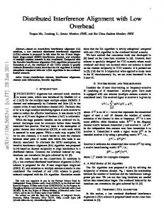
2. EIV-Based System Model In this paper, we consider 𝐾-user IA scheme over MIMO interference channels. As shown in Figure 1, each transmitter and receiver is equipped with 𝑁𝑡 and 𝑁𝑟 antennas, respectively. The channel output at receiver 𝑘 is defined as follows: 𝐾
𝐾
𝑙=1
𝑙=𝑘 ̸
y𝑘 = ∑H𝑘𝑙 x𝑙 + z𝑘 = H𝑘𝑘 V𝑘 s𝑘 + ∑H𝑘𝑙 V𝑙 s𝑙 + z𝑘 ,
(1)
where y𝑘 ∈ C𝑁𝑟 ×1 represents the received signal vector at receiver 𝑘 and x𝑙 ∈ C𝑁𝑡 ×1 is the 𝑁𝑡 × 1 transmitted signal vector at transmitter 𝑙. H𝑘𝑙 ∈ C𝑁𝑟 ×𝑁𝑡 represents the channel fade coefficients from transmitter 𝑙 to receiver 𝑘 for 𝑙, 𝑘 = 1, . . . , 𝐾, where each element is assumed to obey an independent and identically distributed (i.i.d.) complex Gaussian random process with zero mean and unit variance CN(0, 1). z𝑘 ∈ C𝑁𝑟 ×1 is noise vector at receiver 𝑘, which is complex-valued additive white gaussian noise (AWGN) with elements normal distributed as CN(0, 𝜎2 I). V𝑘 ∈ C𝑁𝑡 ×𝑑𝑘 is the TPC matrix with unit-norm and linearly independent columns at transmitter 𝑘, where 𝑑𝑘 is the DoF to meet feasibility of IA scheme at transmitter 𝑘. s𝑘 represents the data streams from transmitter 𝑘, where the transmitted streams are i.i.d. such that 𝐸{s𝑘 s𝐻 𝑘 } = I. Furthermore, the data streams received at receiver 𝑘 can be described as 𝐾
𝐻 𝐻 ̂s𝑘 = U𝐻 𝑘 y𝑘 = U𝑘 ∑H𝑘𝑙 V𝑙 s𝑙 + U𝑘 z𝑘 ,
(2)
𝑙=1
where U𝑘 ∈ C𝑁𝑟 ×𝑑𝑘 is receiving filter matrix with unit-norm and linearly independent columns at receiver 𝑘. In most IA schemes, perfect CSI is assumed. However, CSI is far from being perfect in realistic practical system. We assume that only imperfect estimation of global CSI is
Mathematical Problems in Engineering
3
available at each terminal. The feedback channels are assumed to be error-free. The imperfect CSI model can be quantized according to ̂ 𝑘𝑙 + H ̃ 𝑘𝑙 , H𝑘𝑙 = H
∀𝑙, 𝑘 ∈ {1, 2, . . . , 𝐾} ,
(3)
̂ 𝑘𝑙 is the estimated channel matrix from transmitter 𝑙 where H ̃ 𝑘𝑙 is the CSI error matrix between the true to receiver 𝑘 and H and available information. This error matrix is assumed to be i.i.d. zero-mean complex Gaussian, and ̃ 𝑘𝑘 H ̃ 𝐻 } = 𝜎2 I, 𝐸 {H 𝑘𝑘 ℎ,I
∀𝑘 ∈ {1, 2, . . . , 𝐾} ,
(4)
̃ 𝑘𝑙 H ̃ 𝐻} = 𝜎2 I, 𝐸 {H 𝑘𝑙 ℎ,II
∀𝑙 ≠ 𝑘 ∈ {1, 2, . . . , 𝐾} ,
(5)
̃ 𝑘𝑙 H ̃ 𝐻} = 0, 𝐸 {H 𝑖𝑗
∀𝑘 ≠ 𝑖, 𝑙 ≠ 𝑗,
(6)
2 2 and 𝜎ℎ,II indicate the variance where the parameters 𝜎ℎ,I of error for direct link estimation and interference links estimations [10], respectively. From (3) to (6), we know ̃ 𝑘𝑙 ∼ CN(0, I − 𝜎2 I). If ̃ 𝑘𝑘 ∼ CN(0, I − 𝜎2 I) and H H ℎ,I
ℎ,II
2 2 , 𝜎ℎ,II → 0, then the imperfect CSI model reduces to the 𝜎ℎ,I 2 , case that perfect CSI is available at terminals, and when 𝜎ℎ,I 2 𝜎ℎ,II → 1, it represents that no CSI is available terminals. The 2 2 and 𝜎ℎ,II can potentially have different values parameters 𝜎ℎ,I corresponding to different accuracy of channel estimation of the direct links and that of the interference links. Due to imperfect CSI, then (2) can be written as 𝐾
𝐻 ̂ ̂s𝑘 = U𝐻 𝑘 ∑H𝑘𝑖 V𝑖 s𝑖 + U𝑘 z𝑘
Briefly, the above EIV-based system model can be described by a corrected system of equations [18, 19] Y+ΔY = (H + ΔH)X, where Y ≈ HX and X is the parameter to be estimated, while ΔY and ΔH are the perturbations of Y and H, respectively. As a result, the transmitted signal estimation problem for the IA with imperfect CSI can be defined as a constrained optimization problem: an appropriate cost function depending on the data is minimized over the estimated parameters. The classical method, so-called generalized total least squares (TLS) [18, 20–22], is proposed as a parameter estimation technique for the EIV model when all elements in channel matrices are perturbed by i.i.d. Particularly, the WTLS [19, 23–25] became popular in the mathematics field during this decade since its estimator has a better statistical accuracy under more general noise assumptions. So in the next section we will focus our attention on the WTLS in a realistic CSI error-based interference channel.
3. WTLS-Based Interference Alignment Scheme with Imperfect CSI In this section, the proposed WTLS-based IA scheme will be investigated to solve the IA-based constrained optimization under the condition of imperfect CSI. While minimizing analytically over the correction matrix, the constrained optimization problem can be changed into an equivalently unconstrained optimization problem. And an effective way to set the weights will also be considered. At the end of this section, an iterative algorithm will be presented for the sake of solving the WTLS-based optimization.
𝑖=1
𝐾
𝐻 𝐻 ̂ ̂ = U𝐻 𝑘 H𝑘𝑘 V𝑘 s𝑘 + U𝑘 ∑H𝑘𝑙 V𝑙 s𝑙 + U𝑘 z𝑘 𝑙=𝑘 ̸
(7)
̃ = U𝐻 𝑘 (H𝑘𝑘 − H𝑘𝑘 ) V𝑘 s𝑘 𝐾 + U𝐻 𝑘 (∑H𝑘𝑙 V𝑙 s𝑙 𝑙=𝑘 ̸
𝐾
𝐻̂ ̂ ̂ ̂ ̂s𝑘 + U𝐻 𝑘 (−∑H𝑘𝑙 V𝑙 s𝑙 − z𝑘 ) = U𝑘 H𝑘𝑘 V𝑘 s𝑘 ,
𝐾
̃ 𝑘𝑙 V𝑙 s𝑙 ) + U𝐻z𝑘 . − ∑H 𝑘 𝑙=𝑘 ̸
𝐾
𝐾
𝑙=𝑘 ̸
𝑙=𝑘 ̸
=
(U𝐻 𝑘 H𝑘𝑘
(9)
𝑙=𝑘 ̸
From (7), we hardly find that the IA scheme with CSI error is relative with EIV model. However, when the last two terms on the right-hand part of (7) are moved to the left-hand part, it will be clear that 𝐻 ̃ ̂s𝑘 + [−U𝐻 𝑘 (∑H𝑘𝑙 V𝑙 s𝑙 − ∑H𝑘𝑙 V𝑙 s𝑙 ) − U𝑘 z𝑘 ]
3.1. IA-Based Constrained Optimization with CSI Uncertainties. Looking back on (8), we assume that perfect IA is available and V𝑘 s𝑘 is the true value of its approximation ̂𝑘 s𝑘 (𝑘 ∈ {1, 2, . . . , 𝐾}) such that estimation V
̂ ̂s𝑘 ≈ U𝐻 𝑘 H𝑘𝑘 V𝑘 s𝑘 , where we start with arbitrary TPC matrix and receiving filter matrix. Here we define a measurement data matrix D with CSI errors at 𝑘th receiver 𝐾
̂ s𝑘 − U𝐻 (∑H ̂ 𝑘𝑙 V ̂𝑙 s𝑙 + z𝑘 )] D ≜ [U𝐻 𝑘 H𝑘𝑘 ̂ 𝑘
(8)
𝑙=𝑘 ̸
̃ − U𝐻 𝑘 H𝑘𝑘 ) V𝑘 s𝑘 .
Obviously, from above (8), the terms of interference and 𝐾 𝐾 ̃ 𝐻 noise −U𝐻 ̸ H𝑘𝑙 − ∑𝑙=𝑘 ̸ H𝑘𝑙 )V𝑙 s𝑙 − U𝑘 z𝑘 are considered as 𝑘 (∑𝑙=𝑘 the measurement errors of the interested parameter ̂s𝑘 , while ̃ the CSI error term U𝐻 𝑘 H𝑘𝑘 is considered as the measurement error of the interested parameter U𝐻 𝑘 H𝑘𝑘 . Definitely, this IA system model with imperfect CSI in (8) satisfies the EIV model [18, 19].
=
̂ [U𝐻 𝑘 H𝑘𝑘
̂ ̂ U𝐻 𝑘 H𝑘𝑘 V𝑘 s𝑘 ]
(10)
= [A B] ,
𝐻̂ ̂ ̂ where A ≜ U𝐻 𝑘 H𝑘𝑘 and B ≜ U𝑘 H𝑘𝑘 V𝑘 s𝑘 . According to (3), the measurement data matrix D can be given by
D 𝐾
𝐻̃ ̂ ̂ s𝑘 − U𝐻 = [U𝐻 𝑘 H𝑘𝑘 − U𝑘 H𝑘𝑘 ̂ 𝑘 (∑H𝑘𝑙 V𝑙 s𝑙 + z𝑘 )] 𝑙=𝑘 ̸
4
Mathematical Problems in Engineering ̃ s𝑘 − U𝐻H ̂ 𝑘𝑘 V ̂ 𝑘 s𝑘 ] = [U𝐻 s𝑘 ] − [U𝐻 𝑘 H𝑘𝑘 ̂ 𝑘 H𝑘𝑘 ̂ 𝑘
The first step of WTLS optimization is to minimize the cost function. The minimization with respect to the correction can be carried out as follows:
̃ ̃ B] ̃ = Dtru − D, = Dtru − [A (11) ̃ ≜ U𝐻 H ̃ ≜ ̂s𝑘 − ̃ 𝑘𝑘 , B where Dtru ≜ [U𝐻 s𝑘 ], A 𝑘 𝑘 H𝑘𝑘 ̂ 𝐻̂ ̂ ̃ ≜ [A ̃ B]. ̃ Dtru is the true value of U𝑘 H𝑘𝑘 V𝑘 s𝑘 , and D ̃, 𝑖 ∈ ̃ data matrix D, and D is measurement error. And d 𝑖 𝐻 ̃ ; it is with {1, 2, . . . , 𝑑𝑘 }, is 𝑖th independent column of D covariance matrices (covariance information of measurement error) ̃ ), W𝑖 ≜ cov (d 𝑖
𝑖 ∈ {1, 2, . . . , 𝑑𝑘 } .
(12)
We define an extended matrix of the approximate estimâ 𝑘 s𝑘 tion V ̂ s X V ̂ ≜ [ 𝑘 𝑘] ≜ [ ] , X −I −I
∀𝑘 ∈ {1, 2, . . . , 𝐾} .
(13)
𝑓 (X) =
(14)
Dtru Xtru ≈ 0, with Xtru
∀𝑘 ∈ {1, 2, . . . , 𝐾}
(15)
provided that the initial data matrix D is available and the 𝑑𝑘 error weights information is {W𝑖 }𝑖=1 , corresponding to each row of data matrix D, which totally depends on the quality of CSI. When the data matrix D is confirmed, we set out to seek for a minimal correction ΔD to compensate for the ̃ so that the WTLS optimization [23] measurement errors D, in the presence of a mixture of perfect CSI and CSI error can be defined as min
2 −1 ∑ (√W𝑖 ) Δd𝑖 , 2 𝑖=1
s.t.
(D + ΔD) [
̂ 𝑘 s𝑘 V −I
.. .
] ] ] = 0. ]
(17)
𝐻̂ [Δd𝑑𝑘 X]
̂ is fixed and ̂𝑘 s𝑘 , (𝑘 ∈ {1, 2, . . . , 𝐾}), X For a certain V the constraint of (17) can be treated as linear equations to 𝑑𝑘 optimize variables {Δd𝑖 }𝑖=1 . The set of linear equations in 𝑑𝑘 {Δd𝑖 }𝑖=1 can be expressed as [ ̂+[ DX [ [
̂ Δd𝐻 1 X .. .
] ] ]=0 ]
𝐻̂ [Δd𝑑𝑘 X]
(18) 𝐻
̂ ] , ̂𝐻Δd𝑖 = − [(DX) ⇐⇒ X 𝑖,: ̂ The 𝑖th Let us define residual matrix 𝑄(X) ≜ DX. 𝐻 row of the 𝑄(X) is denoted by 𝑞𝑖 (X); that is, 𝑄𝐻(X) = [𝑞1 (X), 𝑞2 (X), . . . , 𝑞𝑑𝑘 (X)]. As a result, the constraint of (17) can be treated the same way as ̂𝐻Δd𝑖 = − 𝑞𝑖 (X) , X
𝑖 = 1, 2, . . . , 𝑑𝑘 ,
(19)
and thus the constrained optimization problem 𝑓(X) can be separated according to different Δd𝑖 . In this way, the constrained minimization problem (17) is transformed to 𝑑𝑘 independent optimization problems 𝑑𝑘
𝑓 (X) = ∑𝑓𝑖 (X) , 𝑖=1
𝑓𝑖 (X) = min Δd𝑖
2 −1 √ ( W𝑖 ) Δd𝑖 , 2
s.t.
̂𝐻Δd𝑖 = − 𝑞𝑖 (X) , X
𝑑𝑘
̂𝑘 s𝑘 ,ΔD V
̂ Δd𝐻 1 X
𝑖 = 1, 2, . . . , 𝑑𝑘 .
̂ = 0, DX
X0 ] ≜ [ ], ≜[ −I −I
Δd1 ,Δd2 ,...,Δd𝑑𝑘
[ ̂+[ s.t. DX [ [
An alternative expression for the EIV-based system model (8) is
V𝑘 s𝑘
𝑑𝑘 2 −1 ∑ (√W𝑖 ) Δd𝑖 , 2 𝑖=1
min
(20)
𝑖 = 1, 2, . . . , 𝑑𝑘 , (16)
] = 0,
where ΔD𝐻 = [Δd1 , Δd2 , . . . , Δd𝑑𝑘 ]. The optimization ̂𝑘,opt s𝑘 , ΔDopt ) be an optivariables are V𝑘 s𝑘 and ΔD. Let (V mal point of the WTLS optimization problem. Thereupon, ̂𝑘,opt s𝑘 is an optimal WTLS estimation of the true value V𝑘 s𝑘 V and D+ΔDopt is an optimal WTLS estimation of the true data Dtru .
and the optimal correction is −1
̂ (X ̂𝐻W𝑖 X) ̂ 𝑞𝑖 (X) , Δd𝑖,opt = − W𝑖 X
𝑖 = 1, 2, . . . , 𝑑𝑘 . (21)
Employing (21) and the solution of Δd𝑖 can be written as
ΔDopt
[ [ =[ [ [
̂ −1 X ̂ 𝐻 W1 ̂𝐻W1 X) 𝑞1𝐻 (X) (X .. .
] ] ]. ] ]
𝐻 ̂𝐻 ̂ −1 ̂𝐻 [𝑞𝑑𝑘 (X) (X W𝑑𝑘 X) X W𝑑𝑘 ]
(22)
Mathematical Problems in Engineering
5
Hence, the solution of (17) becomes the well-known function [18, 26] as follows: 𝑓 (X) =
=
represent the value of the 𝑙 + 1th iterative result. Thus, we define the approximation function of (24) as follows: 𝑑𝑘
𝑑𝑘
̂ −1 ̂𝐻W𝑖 X) ∑𝑞𝑖𝐻 (X) (X 𝑖=1 𝑑𝑘
∑𝑞𝑖𝐻 (X) 𝑅𝑖−1 𝑖=1
𝐺 (X(𝑙+1) , X(𝑙) ) = ∑ {𝑅𝑖−1 (X(𝑙) ) 𝑞𝑖∗ (X(𝑙) ) 𝑞𝑖 (X(𝑙) )
𝑞𝑖 (X)
𝑖=1
(23)
𝑇
⋅ 𝑅𝑖−1 (X(𝑙) ) [w̃𝑏∗ ̃a∗ − (X(𝑙+1) ) w̃a∗𝑖 ] + 𝑅𝑖−1 (X(𝑙) ) 𝑖
(X) 𝑞𝑖 (X) ,
⋅ 𝑞𝑖∗ (X(𝑙+1) ) a𝑇𝑖 } .
̂𝐻W𝑖 X. ̂ where 𝑅𝑖 (X) ≜ X As a result, the WTLS constrained optimization problem (17) is changed into an equivalently unconstrained optimization problem as follows: min𝑓 (X) . X
(28)
𝑖
(24)
Substituting the expression of 𝑞𝑖 (X) (the expression of 𝑞𝑖 (X) is detailed in the appendix) into (28), thus (28) can be rewritten as 𝑑𝑘
𝑇
𝐺 (X(𝑙+1) , X(𝑙) ) = ∑ {𝑅𝑖−1 (X(𝑙) ) [(X(𝑙+1) ) a∗𝑖 − 𝑏𝑖∗ ] 𝑖=1
𝑇
3.2. Unconstrained Optimization. The second step of the WTLS optimization is to solve the unconstrained optimization problem (24). However, generally, the analytic solution is unavailable [18, 23]. Thus, we propose a numerical method to solve the unconstrained optimization problem. From the unconstrained optimization problem (24), we have the necessary condition for (23) ∇x∗ 𝑓 (X) = 0,
(25)
where ∇x∗ 𝑓(X) is conjugate gradient [27] for the unconstrained optimization problem (24). According to the matrix theory [27, 28], the conjugate gradient which is presented in the appendix is 𝑑𝑘
(26)
𝑇
⋅ [w̃𝑏∗ ̃a∗ − (X(𝑙+1) ) w̃a∗𝑖 ]} . 𝑖
𝑖
Hence, the approximation X(𝑙+1) is defined as the solution of the following equation: 𝐺 (X(𝑙+1) , X(𝑙) ) = 0.
(30)
Substituting (29) into (30), we obtain a system of linear equations with respect to X(𝑙+1) , 𝑑𝑘
𝑇
𝐻
∑ {𝑅𝑖−1 (X(𝑙) ) [(X(𝑙) ) a∗𝑖 − 𝑏𝑖∗ ] [(X(𝑙) ) a𝑖 − 𝑏𝑖 ] ⋅ 𝑅𝑖−1 (X(𝑙) ) (X(𝑙+1) ) w̃a∗𝑖 − 𝑅𝑖−1 (X(𝑙) ) (X(𝑙+1) ) 𝑑𝑘
𝑇
𝑇
(𝑙) 𝐻
⋅ [(X ) a𝑖 − 𝑏𝑖 ] 𝑅𝑖−1 (X(𝑙) ) w̃𝑏∗ ̃a∗ − 𝑅𝑖−1 (X(𝑙) ) 𝑖
𝑖
⋅ 𝑏𝑖 a𝑇𝑖 } 𝑑𝑘
𝑇
∗
⇒ ∑ {𝑅𝑖−1 (X(𝑙) ) [(X(𝑙) ) a∗𝑖 − 𝑏𝑖∗ ] [a𝑇𝑖 (X(𝑙) ) − 𝑏𝑖 ] 𝑖=1
cov (̃a𝑖 )
≜[ ], w̃𝑏𝑖 ̃a𝑖 w̃𝑏𝑖
(X )
𝑖=1
where a𝑖 , ̃a𝑖 , 𝑏𝑖 , and ̃𝑏𝑖 are, respectively, the 𝑖th column of A𝐻, ̃ 𝐻. Note that, in the EIV-based IA system, s𝑘 ̃𝐻, B𝐻, and B A ̂ and X are vectors; thus the solution of X is univariate case. In this case, 𝑅𝑖 (X) is a single component matrix, while 𝑞𝑖 (X), 𝑏𝑖 , and ̃𝑏𝑖 are all single component vectors. The data weights are
w̃a𝑖 w̃a𝑖̃𝑏𝑖
(29)
(𝑙)
⋅ a∗𝑖 a𝑇𝑖 } = ∑ {𝑅𝑖−1 (X(𝑙) ) [(X(𝑙) ) a∗𝑖 − 𝑏𝑖∗ ]
(X) cov (̃𝑏𝑖∗ , ̃a∗𝑖 )]} ,
cov (̃a𝑖 , ̃𝑏𝑖 ) ̃)=[ ] W𝑖 = cov (d 𝑖 cov (̃𝑏𝑖 , ̃a𝑖 ) cov (̃𝑏𝑖 ) ] [
⋅ [(X )
a𝑖 − 𝑏𝑖 ] 𝑅𝑖−1
𝑇
𝑖=1
+ 𝑞𝑖 (X) 𝑅𝑖−1
(𝑙) 𝐻
𝑖=1
∇x∗ 𝑓 (X) = ∑ {𝑅𝑖−1 (X) 𝑞𝑖∗ (X) [a𝑇𝑖 − 𝑞𝑖 (X) 𝑅𝑖−1 (X) X𝑇 cov (̃a∗𝑖 )
⋅ a𝑇𝑖 + 𝑅𝑖−1 (X(𝑙) ) [(X(𝑙) ) a∗𝑖 − 𝑏𝑖∗ ]
𝑇
⋅ 𝑅𝑖−1 (X(𝑙) ) (X(𝑙+1) ) w̃a∗𝑖 − 𝑅𝑖−1 (X(𝑙) ) (X(𝑙+1) ) (27)
𝑖 = 1, 2, . . . , 𝑑𝑘 .
Since there is no closed-form solution for (25), we use an iterative algorithm to solve the problem. Let X(𝑙) represent the approximate value of the 𝑙th iterative result and let X(𝑙+1)
𝑇
𝑑𝑘
𝑇
𝑇
⋅ a∗𝑖 a𝑇𝑖 } = ∑ {𝑅𝑖−1 (X(𝑙) ) [(X(𝑙) ) a∗𝑖 − 𝑏𝑖∗ ] 𝑖=1
∗
⋅ [a𝑇𝑖 (X(𝑙) ) − 𝑏𝑖 ] 𝑅𝑖−1 (X(𝑙) ) w̃𝑏∗ ̃a∗ − 𝑅𝑖−1 (X(𝑙) ) 𝑖
⋅ 𝑏𝑖 a𝑇𝑖 }
𝑇
𝑖
6
Mathematical Problems in Engineering 𝑑
𝑘 2 (𝑙) −1 (𝑙) ⇒ ∑ {𝑅𝑖−2 (X(𝑙) ) a𝐻 𝑖 X − 𝑏𝑖 w̃a𝑖 − 𝑅𝑖 (X )
(7) Define the iterative approximation function as 𝐺(X(𝑙+1) , X(𝑙) ) = 0 and work out X(𝑙+1) .
𝑖=1
(𝑙+1) ⋅ a𝑖 a 𝐻 𝑖 }X
=
𝑑𝑘
∑ {𝑅𝑖−2 𝑖=1
(8) Increase the iteration counter 𝑙 = 𝑙 + 1.
2 (𝑙) (X ) a𝐻 𝑖 X − 𝑏𝑖 w̃a𝑖̃𝑏𝑖 (𝑙)
(9) Repeat steps 5 through X(𝑙) ‖𝐹 /‖X(𝑙+1) ‖𝐹 < 𝛿0 .
until
‖X(𝑙+1)
−
(10) The solution of optimal WTLS estimation is Xopt = X(𝑙) .
− 𝑅𝑖−1 (X(𝑙) ) 𝑏𝑖 a𝑖 } , (31) which is equivalent to a standard system of linear equations 𝐹(X(𝑙) )X(𝑙+1) = 𝑇(X(𝑙) ) where 𝐻 (𝑙) 2 𝐻 a𝑖 X − 𝑏𝑖 (𝑙) − a𝑖 a𝑖 ] , [ 𝐹 (X ) ≜ ∑ w̃a𝑖 𝑅𝑖2 (X(𝑙) ) 𝑅𝑖 (X(𝑙) ) 𝑖=1 [ ] 2 (𝑙) 𝑑𝑘 a𝐻 𝑏𝑖 a𝑖 ] 𝑖 X − 𝑏𝑖 𝑇 (X(𝑙) ) ≜ ∑ [w̃a𝑖̃𝑏𝑖 2 (𝑙) − . 𝑅𝑖 (X ) 𝑅𝑖 (X(𝑙) ) 𝑖=1 [ ] 𝑑𝑘
(32)
On the basis of (29)–(32), we repeat the iterative process and obtain a series of values X(𝑙) and X(𝑙+1) to approximate to accurate value. The iteration continues until ‖X(𝑙+1) − X(𝑙) ‖𝐹 /‖X(𝑙+1) ‖𝐹 < 𝛿0 , and 𝛿0 is a given tolerance. After the iterative process above, we have the final X(𝑙) , approximate to accurate value. Assume that ̂(𝑙) s𝑘 , Xopt = X(𝑙) = V 𝑘
8
𝑘 ∈ {1, 2, . . . , 𝐾} .
(33)
̂𝑘,opt = V ̂(𝑙) (𝑘 ∈ Finally, the estimated TPC matrix V 𝑘 {1, 2, . . . , 𝐾}) can be readily obtained. Hence, the series of ̂𝑘,opt (𝑘 ∈ {1, 2, . . . , 𝐾}) are optimized to estimated values V the true value of the TPC matrix V𝑘 (𝑘 ∈ {1, 2, . . . , 𝐾}) by using WTLS-based IA optimization method. The procedures of the above iteration are outlined in the following algorithm which is presented to solve (24). Algorithm 1 (WTLS-cased IA optimization algorithm). (1) Start with arbitrary TPC matrix V𝑘 and receiving filter matrix U𝑘 . (2) Set the data matrix with CSI error D ≜ [A B] = 𝐻̂ ̂ ̃ ̂ [U𝐻 𝑘 H𝑘𝑘 U𝑘 H𝑘𝑘 V𝑘 s𝑘 ], the measurement error D = 𝐻̃ 𝐻̂ ̂ [U𝑘 H𝑘𝑘 ̂s𝑘 − U𝑘 H𝑘𝑘 V𝑘 s𝑘 ], and the extended matrix ̂ ≜ ̂ 𝑘 s𝑘 : X of the approximate estimation V ̂ 𝑘 s𝑘 V [ −I ] , 𝑘 ∈ {1, 2, . . . , 𝐾}. Caculate the error weights
(11) Finally, according to (13) and constraint of TPC matrix [5], obtain the TPC matrix V𝑘 . Let V𝑘 = ̂𝑘,opt , 𝑘 ∈ {1, 2, . . . , 𝐾}. V (12) Calculate U𝑘 from U𝑘 ∑𝑙=𝑘̸ H𝑘𝑙 V𝑙 = 0 or MMSE method [5]. In this WTLS-based IA optimization scheme, the sum rate result for stream 𝑠 of user 𝑘 is given by (34) where the ̃ 𝑘𝑘 )V𝑘,𝑠 V𝐻 (H𝑘𝑘 − H ̃ 𝑘𝑘 )𝐻 in (34) is the desired signal, (H𝑘𝑘 − H 𝑘,𝑠 and the first, second, third, and fourth terms in (35) represent the interference purely by channel uncertainty, interstream interference, other user interferences, and AWGN, respectively: (𝑠) = log2 det (I 𝑅𝑘,sum
̂ −1 (H𝑘𝑘 − H ̃ 𝑘𝑘 ) V𝑘,𝑠 V𝐻 (H𝑘𝑘 − H ̃ 𝑘𝑘 )𝐻) , +Z 𝑘,𝑠 𝑘,𝑠 where 𝑑𝑘
𝐻 𝐻 ̂ 𝑘,𝑠 = H ̃ 𝑘𝑘 V𝑘,𝑠 V𝐻 H ̃𝐻 Z 𝑘,𝑠 𝑘𝑘 + ∑H𝑘𝑘 V𝑘,𝑡 V𝑘,𝑡 H𝑘𝑘 𝑡=1 𝑡=𝑠̸
𝐾 𝑑𝑙
(3) According to (13), obtain an initial value X(1) of WTLS estimation. (4) Begin iteration, and set the iteration counter 𝑙 = 1. ̂(𝑙) )𝐻W𝑖 X ̂(𝑙) , for 𝑖 = 1, 2, . . . , 𝑑𝑘 . (5) Let 𝑅𝑖 (X(𝑙) ) = (X (6) Compute the residual matrix 𝑄(X(𝑙) ) = AX(𝑙) − B.
(35)
𝐻 + ∑ ∑H𝑘𝑙 V𝑙,𝑡 V𝐻 𝑙,𝑡 H𝑘𝑙 + 𝑃𝑘,noise I. 𝑙=1 𝑡=1 𝑙=𝑘 ̸
V𝑘,𝑠 is the TPC for stream 𝑠 of user 𝑘 and 𝑃𝑘,noise is the power of noise at user 𝑘. The numerator of (34) is the desired signal ̂ 𝑘,𝑠 of (34) is interferences power, while the denominator Z plus noise [11]. And the first, second, third, and fourth terms ̂ 𝑘,𝑠 of the right-hand side of (35) represent the internal in Z perturbation purely by CSI error, interstream interference, other user interferences, and AWGN, respectively. Hence, all sum rate of 𝐾-user IA scheme can be derived easily as follows: 𝐾 𝑑𝑘
(𝑠) . 𝑅sum = ∑ ∑𝑅𝑘,sum
(36)
𝑘=1 𝑠=1
𝑑𝑘 . {W𝑖 }𝑖=1
According to (4) and (5), give information the variances of CSI error, while a convergence tolerance 𝛿0 of WTLS estimation algorithm should also be given.
(34)
3.3. Convergence Issue. In this part, we present the convergence issue of the above iterative algorithm for the WTLS optimization in the previous part. The convergence issue ̂ which equals WTLS estimation X which converges to X0 or X converges to Xtru in probability [23, 29, 30]. Define the variance of each element of measurement error ̃ matrix D 2 2 𝜎𝑖,𝑗 ≜ 𝐸 {𝑑̃𝑖,𝑗 },
𝑖 = 1, 2, . . . , 𝑑𝑘 , 𝑗 = 1, 2, . . . , 𝑁𝑡 + 1. (37)
Mathematical Problems in Engineering
7
We allow some of 𝜎𝑖,𝑗 to be equal to 0. The following assumptions (I) to (VI) are satisfied:
25 100 iterations
(I) For a fixed 𝐽 ⊂ {1, 2, . . . , 𝑁𝑡 + 1}, every 𝑗 ∉ 𝐽 and every 𝑖 = 1, 2, . . . , 𝑑𝑘 satisfy 𝜎𝑖,𝑗 = 0.
(IV) There exists 𝛼 ≥ 2 with 𝛼 ≥ |𝐽| − 1 such that sup(𝑖≥1,𝑗∈𝐽) 𝐸{|𝑑̃𝑖,𝑗 |2𝛼 } < ∞. 𝐻 2 𝐻 𝑟 (V) ∑𝑁 𝑑𝑘 =𝑑0 [𝜆 max (A A)/𝜆 min (A A)] < ∞, 𝑑0 ≥ 1, and 𝑁 is infinite. 𝐻 𝑟 (VI) ∑𝑁 𝑑𝑘 =𝑑0 [√𝑑𝑘 /𝜆 min (A A)] < ∞, 𝑑0 ≥ 1, and 𝑁 is infinite.
Then the WTLS optimization estimation X converges to X0 almost surely (a.s.), as 𝑑𝑘 is large enough. The details of the proofs of convergence and consistency can be found in [23]. And the convergence, availability, and consistency of WTLS optimization estimation are well investigated [18, 23, 29, 30]. From above statements, we find that if 𝑑𝑘 is large enough, estimation X converges to X0 with probability tending to 1. That means the number of rows of the data matrix D must be so large that estimation X converges to X0 with 100% probability. Mathematically, it seems feasible. However, realistically, it is unfeasible in interference management of multiuser MIMO communication system. Since the DoF cannot be infinite. A compromise is reached by the extending the row spacef of the data matrix D 𝐻̂ ̂ U𝐻 𝑘1 H𝑘𝑘 U𝑘1 H𝑘𝑘 V𝑘1 s𝑘
] [ 𝐻 𝐻̂ ] [U H ̂ [ 𝑘2 𝑘𝑘 U𝑘2 H𝑘𝑘 V𝑘2 s𝑘 ] ] [ ] [ .. .. ], [ D≜[ . . ] ] [ 𝐻 [U H ̂ 𝑘𝑘 U𝐻 H ̂ 𝑘𝑘 V𝑘𝑛 s𝑘 ] 𝑘𝑛 ] [ 𝑘𝑛 ] [ .. .. . ] [ .
(38)
where D ∈ C𝑁×(𝑁𝑡 +1) and V𝑘𝑛 and U𝑘𝑛 (𝑛 = 1, 2, . . .) are the arbitrary initialized TPC matrix and receiving filter matrix, respectively. The relevant evaluation of 𝑛 will be discussed in the next section.
4. Numerical Results In this section, simulations are conducted to evaluate the performance of our WTLS-based IA scheme presented in Section 3 for multiuser MIMO interference system with imperfect CSI. Without loss of generality, the CSI errors are assumed to be i.i.d. zero-mean complex Gaussian, and Gaussian input is considered. size of data matrix D is fixed in Figures 2 to 5; that is, the value of 𝑛 in (38) is fixed (here we set 𝑛 = 64), while the WTLS estimation convergence tolerance 𝛿0 = 10−5 . The parameters 𝛼 and 𝛽 indicate the variance of CSI errors for direct link and interference links, respectively. For given
Sum rate (b/s/Hz)
(II) There exists 𝜀 > 0 such that, for every 𝑖 = 1, 2, . . . , 𝑑𝑘 , 𝜆 min (W𝑖 ) ≥ 𝜀2 . ̂ are nonzero vector. (III) The elements of X
20
15
10 100 iterations
5
0
0
5
10
15
20 25 SNR (dB)
WTLS-based IA, 𝛼 = 𝛽 = 0.01 Max SINR, 𝛼 = 𝛽 = 0.01 MMSE, 𝛼 = 𝛽 = 0.01 Iterative IA, 𝛼 = 𝛽 = 0.01
30
35
40
WTLS-based IA, 𝛼 = 𝛽 = 0.1 Max SINR, 𝛼 = 𝛽 = 0.1 MMSE, 𝛼 = 𝛽 = 0.1 Iterative IA, 𝛼 = 𝛽 = 0.1
Figure 2: The sum rate performance of different IA schemes with imperfect CSI for 𝐾 = 3 and 𝑁𝑡 = 𝑁𝑟 = 3 and for the cases 𝛼 = 𝛽 = 0.1 and 𝛼 = 𝛽 = 0.01.
̃ 𝑘𝑘 and H ̃ 𝑘𝑙 randomly according to 𝛼 and 𝛽, we first generate H a zero-mean complex Gaussian distribution from (4) and (5). ̃ 𝑘𝑙 are generated as such, we generate H ̂ 𝑘𝑘 and ̃ 𝑘𝑘 and H After H ̂ H𝑘𝑙 according to (3) to (6), and the true channel is determined by (3). In each plot presented in this section, the sum rate performance is computed via Monte Carlo simulations using 1000 independent channel realizations. Figure 2 shows the sum rate performance of different IA schemes with imperfect CSI for the cases 𝛼 = 𝛽 = 0.1 and 𝛼 = 𝛽 = 0.01, respectively, where we have 𝐾 = 3 users and 𝑁𝑡 = 𝑁𝑟 = 3 antennas at each node. The theoretical maximum DoF which is 4 can be achieved, which means one of the transmitters can obtain 2 DoF and the other two are with 1 DoF. That is to say, this system is unsymmetrical MIMO interference network. It can be observed that the sum rates of all schemes increase as the variance of CSI error decreases. However, the sum rates of all schemes have the error-floor effect because of the internal perturbation purely by CSI error and the interstream interference. From Figure 2, it is seen that the proposed WTLS-based IA scheme outperforms the Max SINR [5], MMSE [13, 14], and Iterative IA [5] (i.e., CJ08 algorithm) schemes for all SNR under different variances of CSI error scenarios. The Max SINR and MMSE schemes show good performance almost comparable to our proposed WTLS-based IA scheme at low SNR. However, as the SNR increases, the sum rates of Max SINR and MMSE schemes increase at slower rate than that of the WTLS-based IA scheme. Particularly, the sum rate of Max SINR scheme degrades to that of MMSE scheme as the SNR increases (these two schemes themselves converge as SNR increases), while both of them still outperform Iterative IA scheme.
8
Mathematical Problems in Engineering 25
3.5 100 iterations
3 Rate per stream (b/s/Hz)
Sum rate (b/s/Hz)
20
15
10 100 iterations
2.5 2 1.5 1
5 0.5 0
0
5
10
15
20
25
30
35
40
0
0
5
10
SNR (dB) WTLS-based IA, 𝛼 = 𝛽 = 0.01 Max SINR, 𝛼 = 𝛽 = 0.01 MMSE, 𝛼 = 𝛽 = 0.01 Iterative IA, 𝛼 = 𝛽 = 0.01
WTLS-based IA, 𝛼 = 𝛽 = 0.1 Max SINR, 𝛼 = 𝛽 = 0.1 MMSE, 𝛼 = 𝛽 = 0.1 Iterative IA, 𝛼 = 𝛽 = 0.1
Figure 3: The sum rate performance of different IA schemes with imperfect CSI for 𝐾 = 3 and 𝑁𝑡 = 𝑁𝑟 = 4 and for the cases 𝛼 = 𝛽 = 0.1 and 𝛼 = 𝛽 = 0.01.
25
Sum rate (b/s/Hz)
20
15
10
5
0
0
5
10
15
20 25 SNR (dB)
Perfect CSI WTLS-based IA, 𝛼 = WTLS-based IA, 𝛼 = WTLS-based IA, 𝛼 = WTLS-based IA, 𝛼 = WTLS-based IA, 𝛼 = WTLS-based IA, 𝛼 = WTLS-based IA, 𝛼 = WTLS-based IA, 𝛼 = WTLS-based IA, 𝛼 = WTLS-based IA, 𝛼 =
30
35
40
𝛽 = 0.01 𝛽 = 0.02 𝛽 = 0.05 𝛽 = 0.1 𝛽 = 0.2 𝛽 = 0.5 0.2, 𝛽 = 0.3 0.2, 𝛽 = 0.5 0.3, 𝛽 = 0.2 0.5, 𝛽 = 0.2
Figure 4: The sum rate of the proposed WTLS-based IA scheme for 𝐾 = 3 users and 𝑁𝑡 = 𝑁𝑟 = 3 with different CSI uncertainties.
K = 3, Nt = 2 K = 3, Nt = 3 K = 3, Nt = 4
15 SNR (dB)
20
25
30
K = 4, Nt = 2 K = 4, Nt = 3 K = 4, Nt = 4
Figure 5: The achievable per-stream rate of the proposed WTLSbased IA scheme for the case 𝛼 = 𝛽 = 0.1.
Generally, Figure 2 shows that there is a considerable gain by using our WTLS-based IA scheme especially under a serious CSI error scenario. Meanwhile, the number of iterations in WTLS-based IA scheme is not more than 10 [19]. It is much less than 100 iterations in both Max SINR and Iterative IA schemes and still less than 16 iterations [13, 14] in MMSE scheme (this MMSE scheme is slightly more complicated as Lagrange multipliers need to be computed to design the transmit beamformers [31]). Figure 3 portrays the sum rate performance of different IA schemes with imperfect CSI for the cases 𝛼 = 𝛽 = 0.1 and 𝛼 = 𝛽 = 0.01, respectively, where we have 𝐾 = 3 users and 𝑁𝑡 = 𝑁𝑟 = 4 antennas at each node. The theoretical maximum DoF is 6 which can be achieved, which means each transmitter is with 2 DoF. That is to say, this system is symmetrical MIMO interference network. Comparing to Figure 2, although the sum rates of all schemes increase as the variance of CSI error decreases, the increasement of the sum rates of all schemes is limited due to the more inter-stream interference with imperfect CSI. It can be observed that the proposed WTLS-based IA scheme still outperforms the other schemes for all SNR under different variances of CSI error scenarios. Our proposed WTLS-based IA scheme can achieve a better performance than the other schemes even at low SNR. Generally, the proposed WTLS-based IA scheme is proven to have good performance under the scenario of symmetrical multiple interstream interference. Figure 4 illustrates the achievable sum rate of the proposed WTLS-based IA scheme for different variances of CSI error, where we have 𝐾 = 3 users and 𝑁𝑡 = 𝑁𝑟 = 3 antennas at each node. It is seen that the achievable sum rate decreases as the variance of CSI error increases. When the variance of
Mathematical Problems in Engineering
9
15
25
10
Sum rate (b/s/Hz)
Sum rate (b/s/Hz)
20
5
0
The variance of CSI error 𝛼 = 𝛽 = 0.1
0
5
10
15
20
25
30
15
10 The variance of CSI error 𝛼 = 𝛽 = 0.01
5
35
40
0
0
5
10
SNR (dB) n=8 n = 16 n = 32
n = 64 n = 128 n = 256
(a) Sum rate versus SNR for 𝛼 = 𝛽 = 0.1
n=8 n = 16 n = 32
15
20 25 SNR (dB)
30
35
40
n = 64 n = 128 n = 256
(b) Sum rate versus SNR for 𝛼 = 𝛽 = 0.01
Figure 6: The sum rate performance of the proposed WTLS-based IA scheme with different sizes of data matrix D for 𝐾 = 3, 𝑁𝑡 = 𝑁𝑟 = 3.
CSI error becomes sufficiently small, the achievable sum rate surely approaches the one with perfect CSI. The starlike and dotted lines represent the achievable sum rate of the proposed WTLS-based IA scheme with different variances of CSI error for direct link 𝛼 and interference links 𝛽, respectively. It can be observed that the sum rate decays as the variance of CSI error only for direct link or interference links increases. The increasement of the variance of CSI error for direct link 𝛼 has a much worse effect on the achievable sum rate than that of the variance of CSI error for interference links 𝛽. This leads to a conclusion that transmitter can achieve a desired transmission rate by allocating minimum required resources according to CSI. Figure 5 describes achievable per-stream rate of the proposed WTLS-based IA scheme versus SNR in 𝐾-user interference channels, where we have 𝛼 = 𝛽 = 0.1. As shown in Figure 5, the achievable per-stream rate monotonically increases, and it saturates in the high SNR regime. However, because of the negative effect of interuser interference, the achievable per-stream rate monotonically decreases as the number of the users increases. It can be also observed that the per-stream rate performance of single stream case for each user is much better than the case of the multiple streams case for each user. The reason is that interstream interference has a negative effect on the rate performance under the CSI error scenario. Generally, under a CSI error scenario (especially a serious CSI error scenario), the more users or antennas the communication system has, the worse the rate performance will be. Figures 6(a) and 6(b) show the sum rate performance of the proposed WTLS-based IA scheme with different sizes of
data matrix D for 𝛼 = 𝛽 = 0.1 and 𝛼 = 𝛽 = 0.01, respectively, where we have 𝐾 = 3 users and 𝑁𝑡 = 𝑁𝑟 = 3 antennas at each node. It can be observed that the sum rate increases as the size of data matrix D magnifies. In other words, when the value of 𝑛 in (38) increases, the sum rate performance of the proposed WTLS-based IA scheme increases. From both Figures 6(a) and 6(b), it can be found that the sum rate performance increases more slowly when the value of 𝑛 is larger than 64. The sum rate begins to converge as 𝑛 = 128. These observations confirm that if the number of rows of the data matrix D is large enough, estimation X converges to X0 with probability tending to 1.
5. Conclusions In this paper, we have considered the sum rate performance of different IA schemes under the condition of CSI uncertainties. We have established an EIV-based system model of IA with imperfect CSI and presented an IA scheme based on WTLS error analysis algorithm for turning the imperfect CSI-based IA optimization (i.e., constrained optimization problem) into an equivalently unconstrained optimization problem in the transmitted signal estimation. Meanwhile, the convergence of the proposed WTLS-based IA scheme is presented as well. Numerical results have shown that the proposed WTLS-based IA scheme can effectively improve the sum rate performance of the MIMO interference channel system compared with several existing IA schemes under different scenarios of CSI error. Numerical results have also shown that the larger the number of rows of the data matrix D is, the higher the accuracy of estimation X is.
10
Mathematical Problems in Engineering
Appendix
Then (A.4) can be rewritten as follows:
Conjugate Gradient of 𝑓(X) 𝑞𝑖𝐻(X), 𝑞𝑖 (X), and 𝑅𝑖 (X) are all the functions of argument X. For the sake of convenience, they can be expressed by X as follows: X ̂ = ([A B] [ ]) = (AX − B)𝑖,: 𝑞𝑖𝐻 (X) = (DX) 𝑖,: −I 𝑖,:
𝑞𝑖 (X) =
= X𝐻a𝑖 − b𝑖 ,
(A.1)
(A.2)
X ̃ )[ ] ̂ 𝐻 W𝑖 X ̂ = [X𝐻 −I] cov (d 𝑅𝑖 (X) = X 𝑖 −I (A.3)
𝐻 −1 𝑑𝑘 𝜕𝑓 (𝑞𝑖 , 𝑅𝑖 ) 𝑑𝑘 𝜕𝑞𝑖𝑇 (X) 𝜕 (𝑞𝑖 𝑅𝑖 𝑞𝑖 ) 𝜕𝑓 (X) = = [ ∑ ∑ 𝜕X∗ 𝜕X∗ 𝜕X∗ 𝜕𝑞𝑖 𝑖=1 𝑖=1 𝐻 −1 𝜕𝑅𝑖𝑇 (X) 𝜕 (𝑞𝑖 𝑅𝑖 𝑞𝑖 ) ], 𝜕X∗ 𝜕𝑅𝑖
𝜕𝑞𝑖𝑇 (X) 𝜕𝑅𝑖𝑇 (X) −1 𝑅 + 𝑞 ]} . (X) (X) 𝑖 𝑖 𝜕X∗ 𝜕X∗
We can derive (A.7) by deducing the terms of 𝜕𝑞𝑖 (X)/𝑑X∗ and 𝜕𝑅𝑖 (X)/𝜕X∗ . Firstly, the derivative term of 𝜕𝑞𝑖 (X)/𝜕X∗ can be derived from (A.2) 𝑑 (X𝐻a𝑖 − 𝑏𝑖 ) 𝜕𝑞𝑖𝑇 (X) 𝜕𝑞𝑖 (X) 𝑇 = [ ] = [ ] = a𝑇𝑖 . 𝜕X∗ 𝜕X∗ 𝑑X∗
𝜕 ([X 𝜕𝑅𝑖𝑇 (X) =[ 𝜕X∗ ={
(A.4)
(A.8)
𝐻
𝜕X∗
𝜕 ([X𝐻 −I]) 𝜕X∗
X ]) −I] W𝑖 [ −I
𝑇
]
𝑇
X
W𝑖 [ ]} −I 𝑇
cov (̃a𝑖 ) cov (̃a𝑖 , ̃𝑏𝑖 ) X } { ][ ] = {[I 0] [ −I } cov (̃𝑏𝑖 , ̃a𝑖 ) cov (̃𝑏𝑖 ) ] } { [
(A.9)
𝑇
where 𝑞𝑖 (X) is a vector, while 𝑅𝑖 (X) is matrix. Note that, ̂ are vectors; thus in the EIV-based IA system, s𝑘 and X the solution of X is univariate case. In this case, 𝑅𝑖 (X) is ̃ are all a single component matrix, while 𝑞𝑖 (X), b𝑖 , and b 𝑖 single component vectors. According to the derivative rules of function with vector argument [27, 28], the 𝜕(𝑞𝑖𝐻𝑅𝑖−1 𝑞𝑖 )/𝜕𝑞𝑖 in the first term of (A.4) can be rewritten as
𝜕𝑞𝑖
⋅ 𝑞𝑖∗ (X) [
Secondly, derivative term of 𝜕𝑅𝑖 (X)/𝜕X can be derived from (A.3)
Obviously, 𝑓(X) is a scalar function. We can treat 𝑓(X) as function with respect to 𝑞𝑖 (X) and 𝑅𝑖 (X). According to the conjugate gradient method for unconstraint optimization and the chain rule of matrix derivative [27, 28], we have
𝜕 (𝑞𝑖𝐻𝑅𝑖−1 𝑞𝑖 )
(A.7)
𝑇
̃) cov (̃a𝑖 ) cov (̃a𝑖 , b X 𝑖 ][ ]. = [X𝐻 −I] [ ̃ , ̃a ) cov (b ̃) cov (b 𝑖 𝑖 𝑖 ] −I [
+
𝑑𝑘
⋅ 𝑅𝑖−1 (X) 𝑞𝑖∗ (X) 𝑞𝑖𝑇 (X) 𝑅𝑖−1 (X)} = ∑ {𝑅𝑖−1 (X) 𝑖=1
𝐻 = (A𝑖,: X − B𝑖,: ) = a𝐻 𝑖 X − b𝑖 , 𝐻 𝐻 (a𝐻 𝑖 X − b𝑖 )
𝑑𝑘 𝜕𝑞𝑖𝑇 (X) −1 𝜕𝑅𝑖𝑇 (X) 𝜕𝑓 (X) ∗ = { 𝑅 𝑞 − ∑ (X) (X) 𝑖 𝜕X∗ 𝜕X∗ 𝑖 𝜕X∗ 𝑖=1
= [cov (̃a𝑖 ) X − cov (̃a𝑖 , ̃𝑏𝑖 )]
= X𝑇 cov (̃a∗𝑖 ) − cov (̃𝑏𝑖∗ , ̃a∗𝑖 ) . Finally, substituting (A.8) and (A.9) into (A.7), we obtain the conjugate gradient of 𝑓(X) 𝑑
𝑘 𝜕𝑓 (X) = ∑ {𝑅𝑖−1 (X) 𝑞𝑖∗ (X) [a𝑇𝑖 ∗ 𝜕X 𝑖=1
𝑇
= [𝑅𝑖−1 (X)] 𝑞𝑖∗ (X) = 𝑅𝑖−1 (X) 𝑞𝑖∗ (X) . (A.5)
According to the derivative rules of function with matrix argument relevant to matrix inverse [28], 𝜕(𝑞𝑖𝐻𝑅𝑖−1 𝑞𝑖 )/𝜕𝑞𝑖𝐻 in the second term of (A.4) can be written as
− 𝑞𝑖 (X) 𝑅𝑖−1 (X) X𝑇 cov (̃a∗𝑖 )
(A.10)
+ 𝑞𝑖 (X) 𝑅𝑖−1 (X) cov (̃𝑏𝑖∗ , ̃a∗𝑖 )]} .
Disclosure Zhengmin Kong and Shixin Peng should be considered cofirst authors.
𝜕 (𝑞𝑖𝐻𝑅𝑖−1 𝑞𝑖 ) 𝜕𝑅𝑖 𝑇
𝑇
= − [𝑅𝑖−1 (X)] 𝑞𝑖∗ (X) 𝑞𝑖𝑇 (X) [𝑅𝑖−1 (X)] = − 𝑅𝑖−1 (X) 𝑞𝑖∗ (X) 𝑞𝑖 (X) 𝑅𝑖−1 (X) .
(A.6)
Conflict of Interests The authors declare that there is no conflict of interests regarding the publication of this paper.
Mathematical Problems in Engineering
Authors’ Contribution Zhengmin Kong and Shixin Peng contributed equally to this work.
Acknowledgment This work was supported in part by the National Natural Science Foundations of China under Grant 61201168.
References [1] S. A. Jafar and S. Shamai, “Degrees of freedom region of the MIMO𝑋 channel,” IEEE Transactions on Information Theory, vol. 54, no. 1, pp. 151–170, 2008. [2] V. R. Cadambe and S. A. Jafar, “Interference alignment and degrees of freedom of the K-user interference channel,” IEEE Transactions on Information Theory, vol. 54, no. 8, pp. 3425– 3441, 2008. [3] T. Gou and S. A. Jafar, “Degrees of freedom of the 𝐾 user 𝑀 × 𝑁 MIMO interference channel,” IEEE Transactions on Information Theory, vol. 56, no. 12, pp. 6040–6057, 2010. [4] H. Yu and Y. Sung, “Least squares approach to joint beam design for interference alignment in multiuser multi-input multioutput interference channels,” IEEE Transactions on Signal Processing, vol. 58, no. 9, pp. 4960–4966, 2010. [5] K. Gomadam, V. R. Cadambe, and S. A. Jafar, “A distributed numerical approach to interference alignment and applications to wireless interference networks,” IEEE Transactions on Information Theory, vol. 57, no. 6, pp. 3309–3322, 2011. [6] L. Zhang, L. Song, M. Ma, Z. Zhang, M. Lei, and B. Jiao, “Interference alignment with differential feedback,” IEEE Transactions on Vehicular Technology, vol. 61, no. 6, pp. 2878–2883, 2012. [7] D. A. Schmidt, C. Shi, R. A. Berry, M. L. Honig, and W. Utschick, “Comparison of distributed beamforming algorithms for MIMO interference networks,” IEEE Transactions on Signal Processing, vol. 61, no. 13, pp. 3476–3489, 2013. [8] Z. Kong, S. Yang, F. Wu, L. Zhong, S. Peng, and L. Hanzo, “An iteratively distributed total-utility mse approach for secure communications in mimo interference channel,” IEEE Transactions on Vehicular Technology. Submitted. [9] S. W. Peters and R. W. Heath Jr., “Cooperative algorithms for MIMO interference channels,” IEEE Transactions on Vehicular Technology, vol. 60, no. 1, pp. 206–218, 2011. [10] H. Farhadi, M. N. Khormuji, C. Wang, and M. Skoglund, “Ergodic interference alignment with noisy channel state information,” in Proceedings of the IEEE International Symposium on Information Theory (ISIT ’13), pp. 584–588, July 2013. [11] J. Park, Y. Sung, D. Kim, and H. V. Poor, “Outage probability and outage-based robust beamforming for MIMO interference channels with imperfect channel state information,” IEEE Transactions on Wireless Communications, vol. 11, no. 10, pp. 3561–3573, 2012. [12] H. Shen, B. Li, Y. Luo, and F. Liu, “A robust interference alignment scheme for the MIMO X channel,” in Proceedings of the 15th Asia-Pacific Conference on Communications (APCC ’09), pp. 241–244, October 2009. [13] H. Shen, B. Li, M. Tao, and Y. Luo, “The new interference alignment scheme for the MIMO interference channel,” in Proceedings of the IEEE Wireless Communications and Networking Conference (WCNC ’10), pp. 1–6, April 2010.
11 [14] H. Shen, B. Li, M. Tao, and X. Wang, “MSE-based transceiver designs for the MIMO interference channel,” IEEE Transactions on Wireless Communications, vol. 9, no. 11, pp. 3480–3489, 2010. [15] H. Huang, V. K. N. Lau, Y. Du, and S. Liu, “Robust lattice alignment for K-user MIMO interference channels with imperfect channel knowledge,” IEEE Transactions on Signal Processing, vol. 59, no. 7, pp. 3315–3325, 2011. [16] B. Xie, Y. Li, H. Minn, and A. Nosratinia, “Adaptive interference alignment with CSI uncertainty,” IEEE Transactions on Communications, vol. 61, no. 2, pp. 792–801, 2013. [17] S. M. Razavi and T. Ratnarajah, “Performance analysis of interference alignment under CSI mismatch,” IEEE Transactions on Vehicular Technology, vol. 63, no. 9, pp. 4740–4748, 2014. [18] I. Markovsky, M. L. Rastello, A. Premoli, A. Kukush, and S. Van Huffel, “The element-wise weighted total least-squares problem,” Computational Statistics & Data Analysis, vol. 50, no. 1, pp. 181–209, 2006. [19] B. Schaffrin and A. Wieser, “On weighted total least-squares adjustment for linear regression,” Journal of Geodesy, vol. 82, no. 7, pp. 415–421, 2008. [20] I. Hnˇetynkov´a, M. Pleˇsinger, D. M. Sima, Z. Strakoˇs, and S. van Huffel, “The total least squares problem in 𝐴𝑋 ≈ 𝐵: a new classification with the relationship to the classical works,” SIAM Journal on Matrix Analysis and Applications, vol. 32, no. 3, pp. 748–770, 2011. [21] X. Fang, “Weighted total least-squares with constraints: a universal formula for geodetic symmetrical transformations,” Journal of Geodesy, vol. 89, no. 5, pp. 459–469, 2015. [22] G. Pan, Y. Zhou, H. Sun, and W. Guo, “Linear observation based total least squares,” Survey Review, vol. 47, no. 340, pp. 18–27, 2015. [23] A. Kukush and S. V. Huffel, “Consistency of elementwiseweighted total least squares estimator in a multivariate errorsin-variables model AX=B,” Metrika, vol. 59, no. 1, pp. 75–97, 2004. [24] A. Amiri-Simkooei and S. Jazaeri, “Weighted total least squares formulated by standard least squares theory,” Journal of Geodetic Science, vol. 2, pp. 113–124, 2012. [25] V. Mahboub and M. A. Sharifi, “On weighted total least-squares with linear and quadratic constraints,” Journal of Geodesy, vol. 87, no. 3, pp. 279–286, 2013. [26] P. Sprent, “A generalized least-squares approach to linear functional relationships,” Journal of the Royal Statistical Society Series B: Methodological, vol. 28, no. 2, pp. 278–297, 1966. [27] X. Zhang, Matrix Analysis and Applications, Tsinghua University Press, Beijing, China, 2004. [28] H. L¨utkepohl, Handbook of Matrices, John Wiley & Sons, Chichester, UK, 1996. [29] A. Kukush, I. Markovsky, and S. V. Huffel, “About the convergence of the computational algorithm for the EW-TLS estimator,” Tech. Rep., Department of Eletrial Engineering, Katholieke Universiteit Leuven, Leuven, Belgium, 2002. [30] S. V. Shklyar, “Conditions for the consistency of the total least squares estimator in an errors-in-variables linear regression model,” Theory of Probability and Mathematical Statistics, vol. 83, pp. 175–190, 2011. [31] C. Wilson and V. Veeravalli, “A convergent version of the Max SINR algorithm for the MIMO interference channel,” IEEE Transactions on Wireless Communications, vol. 12, no. 6, pp. 2952–2961, 2013.
Advances in
Operations Research Hindawi Publishing Corporation http://www.hindawi.com
Volume 2014
Advances in
Decision Sciences Hindawi Publishing Corporation http://www.hindawi.com
Volume 2014
Journal of
Applied Mathematics
Algebra
Hindawi Publishing Corporation http://www.hindawi.com
Hindawi Publishing Corporation http://www.hindawi.com
Volume 2014
Journal of
Probability and Statistics Volume 2014
The Scientific World Journal Hindawi Publishing Corporation http://www.hindawi.com
Hindawi Publishing Corporation http://www.hindawi.com
Volume 2014
International Journal of
Differential Equations Hindawi Publishing Corporation http://www.hindawi.com
Volume 2014
Volume 2014
Submit your manuscripts at http://www.hindawi.com International Journal of
Advances in
Combinatorics Hindawi Publishing Corporation http://www.hindawi.com
Mathematical Physics Hindawi Publishing Corporation http://www.hindawi.com
Volume 2014
Journal of
Complex Analysis Hindawi Publishing Corporation http://www.hindawi.com
Volume 2014
International Journal of Mathematics and Mathematical Sciences
Mathematical Problems in Engineering
Journal of
Mathematics Hindawi Publishing Corporation http://www.hindawi.com
Volume 2014
Hindawi Publishing Corporation http://www.hindawi.com
Volume 2014
Volume 2014
Hindawi Publishing Corporation http://www.hindawi.com
Volume 2014
Discrete Mathematics
Journal of
Volume 2014
Hindawi Publishing Corporation http://www.hindawi.com
Discrete Dynamics in Nature and Society
Journal of
Function Spaces Hindawi Publishing Corporation http://www.hindawi.com
Abstract and Applied Analysis
Volume 2014
Hindawi Publishing Corporation http://www.hindawi.com
Volume 2014
Hindawi Publishing Corporation http://www.hindawi.com
Volume 2014
International Journal of
Journal of
Stochastic Analysis
Optimization
Hindawi Publishing Corporation http://www.hindawi.com
Hindawi Publishing Corporation http://www.hindawi.com
Volume 2014
Volume 2014