EL5206: Computational Intelligence & Robotics. Laboratory – Course Manual. 1
Introduction. Applications which involve the use of mobile, autonomous robots ...
EL5206: Computational Intelligence & Robotics Laboratory – Course Manual 1
Introduction
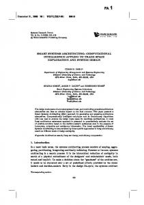
Applications which involve the use of mobile, autonomous robots are countless, varying from surveillance vehicles which carry cameras for internal building security; internal post distribution; under water oil rig maintenance and hazardous environment inspection. All such applications rely on a vehicle being able to automatically sense its surroundings, make intelligent decisions concerning its path towards its goal and then control its wheels/actuators to reach that goal. Extensive research in this field is currently underway in the world today, including here at the Universidad de Chile. The overall EL5206 course is designed to give a practical introduction to computational intelligence and autonomous robotics. The purpose of this part of the course is to give a ‘flavour’ of mobile robotics issues including: • Robot motion and position sensing, • Sensing the environment, • Robot path planning. Hence, various aspects in the understanding and programming of an autonomous mobile robot and its sensors will be addressed in this part of the course. The type of mobile robot to be used is known as a differential drive vehicle, which is capable of linear translation, curved motion, and rotation on the spot. An example of such a mobile robot platform, is shown in the photograph of Figure 1. In this course, the robot will be in simulation form, but has the same kinematic configuration as that of Figure 1. This part of the course will be split into the three sections named above, namely Robot Motion and Position Sensing, Sensing the Environment and Robot Path Planning.
2
Robot Motion and Position Sensing
The aim of this section is to introduce the principles and steps in moving and steering the differential drive type mobile robot. Further, the concept of robot kinematics and inverse kinematics will be introduced, again applied specifically to this type of platform, so that a desired trajectory can be converted into individual wheel/motor commands. A complete understanding of how to influence robot motion can be split into the following two sections.
2.1
Inferring Robot Motion from Wheel Motion - Forward Kinematics
Consider the control of automobile speed by a human operator. The driver decides on an appropriate speed. He observes the actual speed by looking at the speedometer. If he is travelling too slowly, he depresses the accelerator and the car speeds up. If the actual speed is too high, he releases the pressure on the accelerator and the car slows down. It is easy to see here that the
EL5206 - 1
Figure 1: A photograph showing an actual, differential drive mobile robot platform. controlled variable is the car speed; the process plant is the car; the accelerator is the controlling device; the sensor is the speedometer and, of course, the controller is the driver. In contrast, a differential drive robot has the output shaft positions of the motors (which are connected to the wheels) as the controlled variables. This aspect of driving the robot platform differs somewhat from the driver - car example given above. In the driver - car example, the driver sees the overall forward speed of the vehicle, and adjusts it according to the measurement (from the speedometer) of the overall vehicle. He does not need to know or worry about what the individual wheels of the car are doing. For the robot platform, two motor’s are controlled, which rotate the wheels of the platform. These motors/wheels are rigidly connected together by the platform itself, so that individual rotations of each motor’s wheel will end up producing a corresponding motion of the centre point (CP) of the platform. If we want the CP of the platform to move from one position to another (as in the driver - car case), then since we can only control the individual motors, we need to know the exact mathematical relationship between angular wheel rotations (the controlled process) and the movement of the CP of the platform. This relationship is called the kinematics of the vehicle. In particular, given the wheel rotations, we need to calculate the forward kinematics to then calculate the corresponding platform CP motion which would result. 2.1.1
Position Measurement - Wheel Encoders
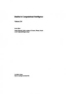
A useful and simple way of monitoring the rotational angle of a wheel, with a computer, is to use wheel encoders. An example of a simple wheel encoder (corresponding to the robot platform in Figure 1) is shown in Figure 2. The reflective disc (rigidly fixed to the inside of each wheel) has non reflective (black) tape spaced evenly over its reflective area. The black plastic sensor, contains an L.E.D. and receiver photo-diode, which receives light reflected back from the L.E.D. EL5206 - 2
Figure 2: A photo of a wheel encoder. The reflective disc (rigidly fixed to the inside of each wheel) has non reflective (black) tape spaced evenly over its reflective area. The black plastic sensor, contains an L.E.D. and receiver photo-diode, which receives light reflected back from the L.E.D. When a reflective segment of the disc is in front of the sensor, the photo-diode output is high, but when black tape is present, the output will be low. When a reflective segment of the disc is in front of the sensor, the photo-diode output is high, but when black tape is present, the output will be low. Hence, the output will be a digital square wave, the frequency of which will increase with increasing wheel speed. In the case of this encoder, every time the computer counts 8 pulses (or 16 pulse edges), one wheel revolution has occurred. Normally such encoders are housed within the motor, and produce thousands of pulses per wheel revolution. The software that you will use allows you to simulate a wheel encoder, attached to each wheel. On a real robot, the controller software monitors these pulses for each wheel, counts them, and turns them into corresponding wheel angles. With knowledge of each wheel’s radius, the displacement of each wheel ∆SL and ∆SR can be found. This is mathematically shown below. 2.1.2
Robot Platform Forward Kinematics
If your vehicle is commanded to move, and you want to keep track of its position, it is first necessary to understand the forward kinematics of the vehicle. This is explained in this section. If the computer is able to record nL/R encoder pulses/edges per wheel revolution from the left and right wheels respectively, then the measurable distance moved through by each wheel after counting these pulses will be ∆SL and ∆SR where: ∆SL = 2πr
nL N
∆SR = 2πr
EL5206 - 3
nR N
(1)
where nL is the number of pulses counted from the left wheel, nR the number from the right wheel, r = radius of the wheels and N = number of encoder pulses/edges per wheel revolution. Referring to Figure 3, to simplify the kinematics, we consider a small manoeuvre, in which the Y w
Differential drive wheels
B R
Instantaneous centre of rotation
O
Initial direction of motion ∆α
∆S
ψ
β
θA
R
A CP X
Figure 3: Mobile platform kinematics (top view of robot). The CP follows an arc ∆S (from A to B) and turns through an angle ∆α for given wheel motions ∆SL and ∆SR . radius of curvature of the turn R of the vehicle is assumed constant. Consider the motion of the centre point (CP) of the robot, which lies half way between the wheels. The distance travelled by this point will be: ∆SL + ∆SR (2) ∆S = 2 and the angle turned through by this point will be ∆α: ∆α =
∆SL − ∆SR w
(3)
where w is the wheelbase length of the vehicle (measured between the points of contact of each wheel with the floor). Figure 3 shows the path followed by the CP of the robot as it turns through an angle ∆α from A to B. We will now determine the changes in x, y and θ during this manoeuvre. In triangle OAB (Figure 3): (AB)2 = R2 + R2 − 2R2 cos ∆α so that:
q
AB = R 2(1 − cos ∆α) EL5206 - 4
(4) (5)
also:
∆S ∆α which can be substituted into equation 5 to give R=
(6)
p
(7)
π π ) + ψ = − θA + ψ 2 2
(8)
∆S 2(1 − cos ∆α) AB = ∆α The angle β in Figure 3 is β = π − (θA + Applying the sine rule in triangle OAB sin ψ sin ∆α R sin ∆α = −→ ψ = sin−1 R AB AB �
Therefore
R sin ∆α π − θA + sin−1 2 AB Substituting equations 6 and 7 into equation 10 gives �
β=
π β = − θA + sin−1 2 Hence p
∆S 2(1 − cos ∆α) sin θA − sin−1 ∆x = −(AB) cos β = − ∆α ∆S 2(1 − cos ∆α) ∆y = (AB) sin β = cos θA − sin−1 ∆α ∆θ = ∆α
(9)
�
sin ∆α p 2(1 − cos ∆α)
p
�
(10)
!
sin ∆α p 2(1 − cos ∆α)
sin ∆α p 2(1 − cos ∆α)
(11)
!!
(12)
!!
(13) (14)
where θA is the initial orientation of the robot platform relative to the x axis. Between them, equations 12, 13, and 14 (together with equations 2 and 3) define the forward kinematics of the vehicle since they relate the measured wheel motions ∆SL and ∆SR to the relative motion of the centre of the vehicle CP in the Cartesian x, y and heading angle θ. This is summarised in Figure 4. The only way in which you can command the simulated robot (and in fact any real robot) is by inputting the left and right wheel rotations ∆SL and ∆SR . The robot will then respond according to Figure 4 and equations 12, 13 and 14. • ASSIGNMENT 1: Determine the necessary parameters from the KiKS software so that you can apply the forward kinematic equations to determine the expected changes in x, y, θ coordinates of the robot, when you enter left and right wheel motion values. • ASSIGNMENT 2: Command the robot wheels to execute several different rotation values in the same time, and calculate the changes in x, y, θ. Verify these changes with the simulation program.
EL5206 - 5
∆SL
∆ SR
∆X Forward Kinematic Model
∆Y
(Eqns. 12, 13 & 14)
∆θ
Figure 4: Forward kinematics. Given the set of wheel rotations (∆SL , ∆SR ) the corresponding relative displacement of a mobile robot (∆x, ∆y, ∆θ) can be calculated.
2.2
Converting the Desired Robot Trajectory into Wheel Motion – Inverse Kinematics
Continuing the above discussion, conversely, if we want to move the CP of the platform from one defined position to another, we need the inverse kinematics to calculate the corresponding wheel rotations necessary to implement that manoeuvre. This inverse kinematic problem is, in general, a very difficult problem to solve. To introduce the concepts to you, the specific kinematics and simplified inverse kinematics of our robot platform only will be addressed. The reason for the difficulty is that given the desired new pose (x, y, θ) of the platform, there are many possible solutions for the necessary left and right wheel rotations to implement it. This is demonstrated in Figure 5. The figure shows that in order to reach B (from A) the robot has several options. It could first rotate on the spot at A to face B and then travel in a straight line towards it (graph 2). Also it could traverse the paths shown in graphs 3 and 4. Although many correct solutions exist, one must be chosen. In robotics research, paths are sought based on some kind of optimality such as minimum fuel (battery power) expenditure, or maximum smoothness. This is beyond the scope of this course, but in general a solution must be chosen as summarised in Figure 6. Calculate the the wheel angles ∆SL and ∆SR which must be input to the wheel controllers to produce the following trajectories: • ASSIGNMENT 3: The platform should move from A to B in Figure 5, by first rotating on the spot at A to face the target B, and then moving in a straight line to it, as in graph 2. • ASSIGNMENT 4: The platform follows a curved smooth trajectory of your choice to reach the target B, in a similar fashion to that shown in graph 3 (more difficult!). Once you have made these calculations, you should implement your algorithm in software.
• ASSIGNMENT 5: Extend the controller program, so that instead of entering the desired wheel angles, the user can now enter the new desired x, y coordinates of the platform, and the platform responds correctly. EL5206 - 6
Y
Y B
B
A
A X
X
Graph 1
Graph 2 Y
Y
B
B
A
A
X
X Graph 4
Graph 3
Figure 5: Many possible inverse kinematic solutions exist for ∆SL and ∆SR for the platform to reach the new coordinates at B. The solid arrow head shows the initial direction of the robot.
Your extension to the program should then correctly implement the block diagram shown in Figure 6 - i.e. the new program automatically calculates the wheel angles ∆SL and ∆SR , based on your inputs x, y and the type of chosen trajectory according to 1 or 2 above. These wheel angles should now be fed directly to the two wheel controllers (which is actually modelled by Figure 4). You will need to use this software to rotate the robot to face certain goal points, and then move towards them, in Part 4 of this course.
3
Sensing the Environment
In reality, a robot becomes useful when it can interact with its environment. For this purpose, exteroceptive sensors are required – sensors which interact with the environment, and make measurements outside of the robot platform. In the KiKS software, the robot is equipped with only very basic sensors, which can detect light levels. The purpose of this section is to understand and calibrate these sensors, so that the robot can estimate the distance to objects around it. In real robotics, these sensors can be cameras, laser range sensors, sonars or radars, or combinations of them and more. EL5206 - 7
∆X
∆ SL Inverse
∆Y ∆θ
Kinematic Model
∆ SR
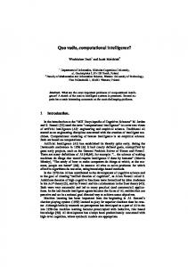
Figure 6: Inverse kinematics. Given the necessary relative displacement for a mobile robot (∆x, ∆y, ∆θ), a corresponding set of wheel rotations must be found (∆SL , ∆SR ). For simplicity, we will use light sources to simulate obstacles, since the sensors can detect these. These light sources can be placed at arbitrary locations around the robot. Figure 7 shows a calibration curve obtained by using the KiKS software to position a light source at a fixed location, and then recording the sensor’s output value, when the robot was at different distances from the light source. Clearly the curve is non-linear, and in order to estimate the range to a
Figure 7: The sensor readings produced by a simulated ambient light sensor, as a function of the horizontal distance between the robot’s centre and a light source. light source (obstacle), it will be necessary to calibrate the sensor output. In order to model the robot’s sensor, it is necessary to perform some simple experiments as follows.
• ASSIGNMENT 6: Using the KiKS software, position a light source at a distance of 180mm along the centre line joining one of its sensors, and the robot’s centre, as shown in figure 8. Then vary the distance r between the centre of the robot and the light source in increments of 20mm towards and away from it. At each location, record the sensor’s output signal. Use the data to plot the output signal versus true range (from the centre of the robot to the light
EL5206 - 8
source) and see if your results match those of figure 7. • ASSIGNMENT 7: Using your results from Assignment 6, determine an approximate mathematical relationship to give the range to the light source as a function of the sensor’s output value.
Another important factor in the modelling of a sensor, is to determine its angular resolution. Again referring to figure 8:
θ r
180mm
Light Source Figure 8: Simple modelling of the robot’s ambient light detection sensor. The diagram shows how variations in the output signal can be determined for different distances r between the centre of the robot and the light source, and different angles of incidence θ.
• ASSIGNMENT 8: With the light source at a distance of 180mm along the centre line joining the sensor, and the robot’s centre, rotate the robot through an angle θ in increments of 1o both clockwise and anticlockwise. Record the sensor’s output signal in each case. Use the data to plot the output signal versus angular offset (from the centre of the robot to the light source). Does the sensor have a narrow or wide beam width? Comment on how useful the sensor is at determining the range and bearing of a point light source.
EL5206 - 9
4
Robot Path Planning - A Simple Artificial Potential Field
A simple path planning method which can be implemented on a mobile platform with sensors which can estimate range, is based on Artificial Potential Fields. An artificial potential field algorithm mimics a real potential field which exists in nature, between, for example, charged particles. Other potential fields which exist in nature are electric potential (voltage), gravitational and magnetic.
4.1
Attraction Towards the Goal
Consider the mobile robot to be a negatively charged particle (e.g. an electron) which can move in the 2D x, y plane. Further, consider a positive charge (e.g. a proton) to be positioned at a predefined goal location x = XG , y = YG . Clearly, as a result of the fixed positive goal charge, a force of attraction will be exerted on the mobile robot (negative charge), thus attracting it towards the goal. This is demonstrated in Figure 9, where the positively charged, fixed goal attractor, produces the resolved forces Xatt and Yatt in the x and y directions respectively. X rob
XG S
F Yrob
x
X att θ rob
Goal
γ
iγ
YG
+
Yatt
Mobile centre line d1 di
−ve Environment
−ve
y
Figure 9: The artificial forces acting on a mobile vehicle. Yatt and Xatt are the components of the attractive force pulling the mobile robot to its goal. F and S are the components of the repulsive force against the mobile robot’s motion, resolved both parallel and perpendicular to its centre line. One way to mathematically model the force of attraction, is to consider the goal and the robot to be connected with an imaginary spring, with spring constant Katt . The force in a spring is proportional to its displacement beyond its equilibrium length. Hence, the force of attraction Patt acting on the robot, which has location coordinates Xrob , Yrob is q
Patt = Katt R = Katt (XG − Xrob )2 + (YG − Yrob )2
(15)
where R is the Euclidean distance between the robot and the goal. This force can be used in terms of its x and y components: Xatt = XG − Xrob
Yatt = YG − Yrob
EL5206 - 10
(16)
4.1.1
Limiting the Attractive Force
It can be seen from equation 15 that if the robot is far from the goal, R and hence Patt become very large. This would mean that the attractive force would make any repulsive forces insignificant, which may result in the robot moving in a straight line towards the goal, and colliding with obstacles. Therefore, this force should be limited, and one way to do this is to impose a limit on R say Rmax , such that if R > Rmax the attractive force saturates to a constant. Hence, equation 15 should be replaced with: R =
q
(XG − Xrob )2 + (YG − Yrob )2
if
R ≤ Rmax :
else if R > Rmax :
Patt = Katt R Patt = Katt Rmax
(17)
Rmax can be set as a distance from the target at which the robot should start to decelerate towards the goal (e.g. 50cm). In the case of R > Rmax , the attractive force components in the x and y directions become: Xatt = Katt
Rmax (XG − Xrob ) R
Yatt = Katt
Rmax (YG − Yrob ) R
(18)
else they are given by Equations 16.
4.2
Repulsion Away from Obstacles
Now consider the range samples, estimated by the robot’s environmental sensors (as in Part 3). By modelling each range sample as fixed negative charges, at their estimated locations, forces of repulsion will result, which tend to push the robot away from them. Figure 9 shows the sum of the repulsive forces F and S resolved along, and perpendicular to, the mobile robot’s centre line respectively. To determine the repulsive forces F and S in Figure 9 we consider each sensor range sample (negative charge, shown as small red crosses in Figure 9) at a radial distance di from the centre of the mobile robot. Hence the force of repulsion between the ith data sample and the mobile robot can be modelled as 1/d2i . This is known as inverse square repulsion and models the way in which real charged particles repel one another. Each of these repulsive forces is resolved parallel and perpendicular to the mobile robot’s centre line and then summed to produce F and S in Figure 9. Hence F and S are given by: (2π/γ)
F =
X i=1
(2π/γ)
S=
X i=1
1 cos(iγ) d2i
(19)
1 sin(iγ) d2i
(20)
where γ = the angle between sensors i and i + 1 around the circumference of the robot platform, di the ith range estimate and i is an integer. Forces F and S can then also be resolved along the x and y axes to give the resolved forces of repulsion Xrep and Yrep : Xrep = Krep F cos θrob
Yrep = Krep S cos θrob
where Krep is a repulsive force constant. EL5206 - 11
(21)
4.3
Path Planning
Based on the overall imaginary force acting on the robot, a path can now be planned. The overall imaginary forces in the x and y directions are given by Px and Py respectively, where: Px = Xatt − Xrep
Py = Yatt − Yrep
(22)
and the magnitude of the overall resultant force P acting on the robot is given by P = and its direction ζP relative to the x axis is:
q
Px2 + Py2
(23)
Py Px
(24)
ζP = tan−1
�
�
The resultant force magnitude and angle can now be used to guide the robot. A simple way to do this is to command the robot to turn on the spot so that it faces the direction of the resultant force ζP , and then command it to move forward in a straight line at a speed proportional to the resultant force P . The robot should then move at this speed for a very short time, until it is ready to sense the environment again, from a new position. Clearly the shorter this time is, the better the calculations will be, at the expense of computational expense. Hence, this requires us to provide signals to the robot’s wheels, based on the inverse kinematics of Graphs 1 and 2 in Figure 5.
• ASSIGNMENT 9: Write a software program, in which you can choose a start and goal coordinate for the robot. In your program, you should also be able to locate obstacles for the robot to avoid. You could use the light sources for this, since the robot’s sensors can detect the signal from these. • ASSIGNMENT 10: Extend the program, so that at a given robot location, it calculates the attractive force Patt . Also, based on your sensed range calibrations of Section 3 detected from the obstacle light sources, extend the program so that it calculates the repulsive forces Xrep and Yrep . • ASSIGNMENT 11: Use the calculated attractive and repulsive forces to turn the robot in the direction of the resultant force acting on it. Then command the robot to move at a speed proportional to P in the direction of the resultant force, for a short time. • ASSIGNMENT 12: After this manoeuvre, repeat Assignment 11 until the robot converges to a new position, and P reaches zero. • ASSIGNMENT 13: Adjust the values of Katt , Krep and Rmax and note their affect on the algorithm.
EL5206 - 12
4.4
The Effect of Katt and Krep
The constant Krep has been introduced in order to show the effect of the repulsive force field. As an example, the left hand diagram in Figure 10 shows the vehicle tracking a target with Krep set to unity. In each figure, each triangle represents a location of the robot in which the
Figure 10: Plan view of the paths taken by the mobile robot (represented as a triangle) when Krep is set to unity (left hand figure) and when Krep is set to 7.0 (right hand figure). In each case the same start (upper right triangle) and target coordinates were used, the target being shown by a cross (+) in both figures. algorithm was executed. The solid lines represent a plan view of the simple environment (walls and a pillar). The scan results taken from the mobile robot’s final position are shown in each cased. Each small cross corresponds to a range sample, recorded from the robot’s final pose. The mobile robot follows a slightly curved path as depth readings from the on board sensor are allowed to influence the vehicle’s controller to the maximum effect, without causing any false minima within the workspace. In the right hand figure, Krep is set to 7 and the surroundings are therefore allowed more influence upon the path of the mobile. Note the effect upon the path, particularly near the target where the effect of the sensor data, forces the mobile robot away from the target. Figure 11 shows the same start and end coordinates with Krep set to 1000 so that the repulsive forces dominate the controller’s input. The ‘over cautious’ nature of the mobile robot’s path EL5206 - 13
Figure 11: Krep is set to a large value (1000) thus making the environmental repulsive forces dominate the path of the vehicle. The mobile robot attempts to follow the Voronoi path keeping itself equidistant from sensed obstacles. A false minima has been generated as the overall force on the vehicle reaches zero at the end of the path shown. The cross (+) shows the target. can clearly be seen. The mobile robot attempts to reach the ‘safety optimal’ Voronoi Path, as it tries to position itself at equal distances from all obstacles. Convergence of the robot to its goal is no longer guaranteed as the repulsive forces now balance the attractive forces. The theory presented here can be used to complement other navigation strategies. If the targets are placed in safe and reachable positions the potential field algorithm is more likely to produce paths which converge to the goal, whilst steering away from obstacles. We cannot rely solely upon the repulsive force field for navigation, but it can be used to influence a path planner in order to produce smooth paths for the vehicle.
• ASSIGNMENT 14: Write a brief report on your software and the results, showing your answers to the above assignments including methods, software, results and conclusions. The report should include figures showing results from the KiKS software. It should be no longer than a total of 10 pages.
EL5206 - 14