Electrode Boundary Conditions and Experimental ... - Semantic Scholar

1180

IEEE TRANSACTIONS ON MEDICAL IMAGING, VOL. 25, NO. 9, SEPTEMBER 2006

Electrode Boundary Conditions and Experimental Validation for BEM-Based EIT Forward and Inverse Solutions Saeed Babaeizadeh, Student Member, IEEE, Dana H. Brooks*, Senior Member, IEEE, David Isaacson, Member, IEEE, and Jonathan C. Newell, Member, IEEE

Abstract—In this paper, we present theoretical developments and experimental results for the problem of estimating the conductivity map inside a volume using electrical impedance tomography (EIT) when the boundary locations of any internal inhomogeneities are known. We describe boundary element method (BEM) implementations of advanced electrode models for the forward problem of EIT. We then use them in the inverse problem with known internal boundaries and derive the associated Jacobians. We report on the results of two EIT phantom studies, one using a homogeneous cubical tank, and one using a cylindrical tank with agar conductivity inhomogeneities. We test both the accuracy of our BEM forward model, including the electrode models, as well as our inverse solution, against the measured data. Results show good agreement between measured values and both forward-computed tank voltages and inverse-computed conductivities; for instance, in a phantom experiment, we reconstructed the conductivities of three agar objects inside a cylindrical tank with an error less than 2% of their true value. Index Terms—Boundary element method, electrical impedance tomography, electrode models, experimental validation, inverse problem.

I. INTRODUCTION

E

STIMATING the conductivity map inside a volume from electrical measurements on its surface an imaging modality known as electrical impedance tomography (EIT), has been a subject of much recent interest (for a recent review, see [1]). Possible biomedical applications include monitoring cardiac and pulmonary function [2], detection and characterization of tumors [3], monitoring cancer ablation procedures [4], and Manuscript received March 6, 2006; revised May 15, 2006. The work of S. Babaeizadeh and D. H. Brooks was supported in part by the by the Center for Integrative Biomedical Computing, NIH NCRR Project 2-P41-RR12553-07 and in part by the Center for Subsurface Sensing and Imaging Systems (CenSSIS), under the Engineering Research Centers Program of the National Science Foundation under Award EEC-9986821. The work of D. Isaacson and J. C. Newell was supported by in part by CenSSIS and in part by the National Institute of Biomedical Imaging and Bioengineering under Grant R01-EB000456. Asterisk indicates corresponding author. S. Babaeizadeh is with the Advanced Algorithm Research Center (AARC), Philips Medical, Thousand Oaks, CA 91320 USA (e-mail: saeed.babaeizadeh@ philips.com). *D. H. Brooks is with the Department of Electrical and Computer Engineering, Northeastern University, Boston, MA 02115 USA (e-mail: brooks@ ece.neu.edu). D. Isaacson is with the Department of Mathematical Sciences, Rensselaer Polytechnic Institute, Troy, NY 12180 USA (e-mail: [email protected]). J. C. Newell is with the Department of Biomedical Engineering, Rensselaer Polytechnic Institute, Troy, NY 12180 USA (e-mail: [email protected]). Digital Object Identifier 10.1109/TMI.2006.879957

building forward models for bioelectric field inverse problems such as electroencephalography/magnetoencephalography (EEG/MEG) [5] and electrocardiography/magnetocardiography (ECG/MCG). A variety of nonclinical applications of EIT are also possible, including imaging multiphase fluid flow [6]. EIT is an ill-posed inverse problem, meaning that large changes in impedance at the interior of the object may result in only small changes to the electrical measurements on its surface, and thus the inverse problem is not stable to data perturbation or model errors [1]. To detect small size impedance variations within the object, effectively providing good spatial resolution, we need to estimate a large number of conductivity parameters in the inverse problem, which further reduces the stability of the solution algorithm. Therefore, there is a tradeoff, in the general case, between spatial resolution and stability. The fact that the conductivities depend nonlinearly on the measured quantities makes this trade-off even more difficult. The ill-posedness of the problem makes it unlikely that EIT images, even with many electrodes, can achieve resolution comparable to that of computed tomography (CT) or magnetic resonance imaging (MRI) images. However, EIT is low-cost, noninvasive, and provides information about the electrical parameters of the body, information that cannot be obtained easily, if at all, by these other methods [7]. In a particular class of EIT applications, one can partially address the ill-posedness by modeling the volume as being composed of a relatively small number of piecewise-constant regions and assuming that one can obtain the geometry of these regions ahead of time (e.g., through application of some anatomical imaging method such as CT or MRI). In that case, the unknowns are reduced to one parameter value per region. As an example, this approach could be used for the bioelectric field inverse problems mentioned above. These problems require one to construct a forward model of the volume conductor; this model in turn depends on the distribution of conductivity in the volume. One can simply use typical conductivity values from the literature; however, different studies have reported different conductivity values for various types of human tissue [8]. When accurate conductivity values are important, and anatomical imaging modalities are available, then one could in principle use EIT to find the conductivities based on a geometric model of internal inhomogeneity (e.g., organ) boundaries obtained from an anatomical image. The forward problem of EIT involves constructing a forward model to calculate the potentials (or currents) produced on the

0278-0062/$20.00 © 2006 IEEE

BABAEIZADEH et al.: ELECTRODE BOUNDARY CONDITIONS AND EXPERIMENTAL VALIDATION FOR BEM-BASED EIT FORWARD AND INVERSE SOLUTIONS 1181

boundary when currents are injected (or voltages are applied) on the same boundary. There are a number of variations of EIT that depend on whether one injects current (and measures voltage) or applies voltage (and measures current), and whether one uses the same or different electrodes for these two purposes. In the approach we use here, called adaptive current tomography (ACT) [9], we apply a set of current patterns to an array of electrodes located on the object surface and record the resulting voltage with those same electrodes. This model is typically obtained by assuming the geometry and conductivities are known and solving Laplace’s equation for the potential in the interior of the volume with appropriate boundary conditions. Since an analytical solution of Laplace’s equation is only possible for simple regular geometries, in general we need to solve it numerically. One numerical method which has been widely studied for the EIT problem is the finite-element method (FEM) [10], [11]. Another numerical method which has been used for solving Laplace’s equation in the interior of the volume with appropriate boundary conditions is the boundary element method (BEM) (also known as the boundary integral method) [12]. The BEM requires calculating only boundary values, rather than values throughout the computational volume. One advantage of BEM is that only the surfaces of the objects need to be discretized, in contrast to the need to discretize the whole volume for FEM. Thus, with BEM, we can avoid the need to construct a complete volume mesh, which respects irregular internal boundaries for complicated three-dimensional (3-D) objects, which can be a time-consuming exercise. There has been much previous work on BEM methods for torso and head internal source bioelectric field problems [13], [14]. One difference between EIT and those problems is that for EIT the known boundary condition and the measurement boundary condition are on the same surface, while in internal source problems the first of these boundary conditions is on either the heart or cortical surface, and the second on the external surface. Another difference is that the known boundary condition is Neumann (representing the current sources) not Dirichlet (known potentials). Two approaches based on BEM to solve the EIT problem were reported in [15], [16]. In [17]–[19], we described and compared BEM and FEM approaches to solve the known-geometry 3-D EIT inverse problem. In that work, it was assumed that the electrodes were very small (point electrodes), so that one could assume the gradient of the potential was nonzero only at isolated points on the outer surface under those point electrodes. Obviously in practical situations this is not a valid assumption; no matter how small the electrodes are, they cover a part of the surface. Moreover, it has been shown in [20] that the resolution of an EIT system improves if one uses electrodes that fill as much as of the outermost surface as possible. The use of such large electrodes changes the boundary conditions to be imposed on the EIT problem. A sequence of such advanced electrode models was first introduced by Cheng et al. in [21]. These models, in order of increasing fidelity (and complexity), are generally known as the continuum, gap, ave-gap, shunt, and complete models. The continuum model assumes the current density on the entire outer surface is known; in effect, each point has its own “differential electrode.” The gap electrode

model is a refinement of the continuum model which accounts for the discreteness of the electrodes. However, metal electrodes provide a low-resistance path for the current, so that all the nodes under each electrode have (almost) the same potential. One can approximate this effect by adding a postprocessing step to the gap model that replaces the nonuniform voltages over the electrodes by an average value, called the ave-gap model. Enforcing this constraint more accurately requires reformulating the problem, and the result is called the shunt model. Modeling in addition the contact impedance between the electrode and the body results in the complete model. These boundary conditions require particular treatment in any numerical method; for instance, an FEM implementation can be found in [22]. In this paper, we present a method to impose these advanced electrode boundary conditions in a 3-D BEM model. We then present results of validation experiments recently carried out at the Electrical Impedance Imaging Laboratory, Rensselaer Polytechnic Institute, Troy, NY, using two different phantom tanks. The first set of experiments we present was performed by Choi et al. [23] using a rectangular box with electrode arrays on the top and the bottom planes, as a simplified model of a mammography geometry, to validate an analytical forward model for the corresponding geometry with a homogeneous conductivity distribution. These investigators generously allowed us to use both their analytical solution and their experimental data to validate our numerical forward solution. In addition, to simulate a geometry more similar to a torso and to test the effect of conductivity inhomogeneities, we carried out another set of experiments using a cylindrical phantom tank and agar “internal organs.” We report here on the results for both homogeneous and inhomogeneous conductivity distributions. We have previously presented a part of this work at the 2005 BEM/NFSI Conference [24]. II. INCORPORATING THE ADVANCED ELECTRODE MODELS INTO BEM-EIT In the forward problem, we assume the geometry and conductivities are known and model the relation between the current injected by electrodes placed on the outermost surface and the potential distribution on the same surface. Using the BEM-based method, this relationship is represented as (1) where , usually known as the Dirichlet to Neumann map, is a dense matrix that relates , the potential distribution at the nodes on the outermost surface, to , the current distribution of those same nodes. is a function of the geometry and conductivities of the entire volume, as well as of the boundary conditions. For the gap electrode model in BEM, is known, and thus we can directly use (1) to find . A. Shunt Model In this model, the number of unknown voltages decreases because we now only have one unknown voltage per electrode. However, the number of unknown currents increases because, in

1182


contrast to the gap model, we no longer know the current density applied at each boundary node. If we denote the number of electrodes by , the total number of mesh nodes on the outermost surface by , and the total number of mesh nodes on the outermost surface which are under the electrodes by , by reordering the system of BEM (1) so that nodes under electrodes are grouped together, and likewise with those nodes not under electrodes, we get (2) Here, is a vector of the current densities at the surface nodes not under the electrodes, and, therefore, is equal to the zero is the vector of current densities at the nodes vector, while under the electrodes and is unknown. Thus (3) We can augment this system with equations that each relates the value of the current density at the nodes under one electrode to the known input current on that electrode. The total cur, is equal to the integral of the current going into electrode , where rent density over that electrode, i.e., is the surface area of electrode . We can write a discretized approximation to this equation using an appropriate set of basis functions as

(4)

where is the number of nodes under electrode , and is an element of a weighting vector which relates the current density of the nodes under electrode to the current applied to that electrode. ’s in this equation, we numerically compute To find the the integral on the surfaces of triangles under the electrode in a manner consistent with our numerical solution to the BEM integrals. In particular, we use a linear interpolating polynomial basis expansion function, first developed by Cruse [25], so that at any point on the triangle we can approximate the current , i.e., the normal vector of the potendensity tial gradient multiplied by the conductivity at that point, as a weighted sum of the values at the three vertices. Using this general approximation, we can write for the current density at any point

(5)

is the value of the current density at vertex m of the triwhere can be evaluated using angle. The interpolating polynomial the method presented in [25].

With

so defined, it is possible to write for electrode

(6)

is the number of triangles under electrode which where share the common vertex , and is the vertex number of each triangle. We can evaluate the integral on the right side of (6) using either analytically integrated elements [26] or a method of numerical quadrature such as Radon’s seven-point formula [27]. We note that the form of (6) is the same as that of (4). Although separation of geometrical coefficients from current density values is achieved, it is impossible to write an analytical expression for the weighting coefficients since the relationship between and is a function of how the surface has been triangulated. However, one can keep track of all the coefficients applied to the potential at each node in a running sum, to produce a weighting vector. By inserting zeros in the positions of this vector corresponding to the mesh nodes under the other which electrodes, we can construct a weighting vector relates the current density of the nodes under all the electrodes to the current applied to electrode . Performing similar computations for all electrodes, we construct a matrix which relates the current density value at all the nodes under the electrodes to the current applied to those electrodes

(7) In the shunt model, as mentioned, all the nodes under one electrode have the same potential. To apply this boundary condition, we can equate the potential at one node on a given electrode to the potential at every other node on the same electrode by simply setting the difference of the potential at each such pair of nodes to zero. Noting that equating the potentials at all vertices of all the triangles under each electrode makes the potential everywhere under that electrode equal under our approximation, this imposes the correct boundary condition. The difference coand that constrain the voltages under an elecefficients trode are stored in matrix

(8) Equations (3), (7), and (8), together, make the following square system of equations:

(9)

We can rearrange terms to solve directly for for instance via Gaussian elimination. If we are only interested in the electrode voltages, we can further speed up the process by only solving for the corresponding elements of . To solve the inverse problem using the BEM, it is useful to obtain the Jacobian matrix [17], [18]. To do so, we differentiate


(3), (7), and (8) with respect to (the constant conductivity of any of the distinct regions), and then rearrange to get

(10) Solving this system gives (11) where

is found by solving the system of (9).

B. Ave-Gap Model As mentioned in Section 1, the ave-gap model is an intermediate approximation to the shunt model. To apply this model to our boundary element solution, we can compute the voltages on electrodes as

(12) is the same as that of matrix in (7) but where each row of divided by the number of nodes on the corresponding electrode, and is the potential computed using the gap model. C. Complete Model Since the complete model takes into account the contact impedance, the potentials of the nodes under an electrode do not have to be the same. Instead the following equation is valid for each point under the given electrode: (13) where is the effective contact impedance, and is the voltage of the electrode. To include this effect, we replace the lower left corzero matrix in (10) with a matrix , where each row of responds to one electrode and has the correct value of the coror ) for the nodes responding contact impedance (times under that electrode, and 0’s elsewhere. Again the coefficients and in are used to set to zero the difference of in (13) at each pair of nodes which are on the same electrode, and can speed up the and again we can solve this system for computations when only the electrode voltages are of interest. To compute the Jacobian, we follow the method described above, but with the modified system of equations, to get and then from (13) we have (14) III. EXPERIMENTAL VERIFICATION A. Analytical Solution and Experimental Data for a Homogeneous Cube In [23], Choi et al. presented an analytical solution for a homogeneous cube based on the ave-gap electrode model and

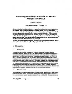
Fig. 1. Cubical test tank and its triangular surface mesh. (a) Test tank used in the experiments; two 4 4 electrode arrays are located on left and right side walls. For each planar electrode array, the electrodes are numbered consecutively from left to right and top to bottom, as indicated on Fig. 1(b). (b) Surface mesh made for the test tank. It has 1016 nodes and 2028 triangles with each electrode covering nine nodes and eight triangles.

2

compared their analytical solution with experimental results. We used both their analytical solution and their experimental data to validate our numerical forward solution. The Plexiglas test tank used in this experiment is shown in Fig. 1(a). It is filled with a 367 mS/m saline. It has inner dimensions of 50 mm on a side. The effective height is determined by the level of saline solution. Planar electrode arrays are located on the left and right array of copper side walls. Each electrode plane consists of electrodes fabricated on a printed circuit board (PCB). The total number of electrodes is 32; each is 10 mm 10 mm and the gap between them is 2 mm. For each planar electrode array, the electrodes are numbered consecutively from left to right and top to bottom, as indicated in Fig. 1(b). The ACT3 system [28] was used in this experiment to apply the current and measure the voltage. To use the BEM-based solution, we constructed a triangular mesh for the test tank, shown in Fig. 1(b). Shaded regions represent the electrodes. The mesh has 1016 nodes and 2028 triangles with each electrode covering nine nodes and eight triangles. To compare the different forward solutions, in addition to visual inspection of the results, we computed the signal-to-noise ratio (SNR), defined as

(15) Note that when we are comparing either the BEM or analytical solution with the measurement data, denotes the potential at electrode predicted either by the BEM model or the analytical solution, the experimentally measured potential at electrode on the test tank, and the number of electrodes. When we compare the analytical solution with the BEM forward solution, denote the potential at electrode predicted by the we let BEM forward model, and the result of the analytical solution. On the plots, we also report the value of this error in terms of %norm error, where

% (16)

1184

Fig. 2. Measured voltages and results of the analytical and BEM solutions with the ave-gap electrode model for two different current patterns applied to the homogeneous cubical tank shown in Fig. 1.

We used the same current patterns in the BEM model as those Choi et al. used for their experiments [23]: the eigenfunctions of the current-to-voltage map for a homogeneous medium. Fig. 2 shows the measured potentials and results of both analytical and BEM ave-gap solutions for two of the applied current patterns. It is seen that the %norm error between the BEM solution and analytical solution varies for different current patterns; for example, it is 8.95% for the lower frequency current pattern 1 and 2.16% for the higher frequency current pattern 2. Nevertheless, we observe that both solutions result in a comparable match with the measured potentials. Using the BEM shunt model results in a noticeable improvement, as seen in Fig. 3. Since the analytical solution with the shunt model was not available, we display the analytical solution with the ave-gap model instead to illustrate the improvement. We observe that now the BEM solution with the shunt electrode model results in a better match to the measured potentials than the analytical solution with the ave-gap electrode model. To use the complete model, we need to know the contact impedance of the electrodes. Since actual values were not available to us, we assumed it to be constant and experimented with different values. We observed that different values of contact impedance improved the results for some current patterns while making the results worse for other current patterns. One way to choose a constant contact impedance for all the electrodes is to use the value of contact impedance which minimizes the mean square value of the difference between the measurement and BEM solution across all the current patterns. Results using


Fig. 3. Measured voltages and results of the BEM solution with the shunt model, and analytical solution with the ave-gap model, for two different current patterns applied to the homogeneous cubical tank shown in Fig. 1.

this value for the complete model were only slightly different from using the shunt model for this experiment. B. Experiments With a Cylindrical Tank We also validated our BEM-based forward models by comparing the electrode voltages predicted by the model to the experimental results obtained using a cylindrical phantom tank. Fig. 4 shows the cylindrical test tank, agar “lungs” and “heart,” and the ACT3 system used to apply the current and measure the voltage. This tank is also made of plexiglas and has an inner diameter of 290 mm. 256 stainless-steel electrodes, each 25.4 mm 25.4 mm in size, are arranged in eight rows, with the bottom layer having its lower edge 240 mm above the tank bottom. The electrodes occupy 225 mm of vertical extent (eight rows of electrodes and the seven intervening gaps). The interelectrode gaps are the same size horizontally and vertically. For our experiments, we used 32 of the 256 electrodes configured as four rows of eight equally spaced electrodes. The unused electrodes were covered with plastic tape to prevent them from changing the boundary conditions. The electrodes are numbered at top, as consecutively around each row starting from the indicated on Fig. 4(c). The voltages generated on the electrodes depend on the current pattern applied. Since the measured voltages are to be used in the inverse solution, it is desirable to apply currents that result in the largest possible voltages. Previous studies have shown that the current patterns which maximize this voltage correspond to the eigenfunctions of the current-to-voltage map. For unknown conductivity distributions, these patterns can be obtained iteratively by an adaptive process [20]. However, in this work, we


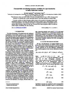
Fig. 4. Experimental apparatus at RPI, geometry and surface mesh of the cylindrical test tank. (a) ACT3 and the cylindrical tank. (b) Agar “lungs” and “heart” in the tank. (c) Triangular mesh made for the test tank: 1622 nodes and 3240 triangles, each electrode covering 6 nodes and 4 triangles. The electrodes are numbered consecutively around each row starting from the x at top, as indicated on figure. (d) Cylindrical tank and the internal agar “lungs” and “heart” (dimensions are in millimeters); left: top view, right: side view.

+

used a set of simpler canonical current patterns which are optimal for circular shapes [1]. In our first experiment, we filled the tank to a height of 540 mm with a homogeneous saline solution with conductivity of 410 mS/m. For the BEM-based forward model, we discretized the tank with a triangular boundary mesh with 1622 nodes and 3240 triangles. Each electrode covered six nodes and four triangles of this surface mesh [see Fig. 4(c)]. For each current pattern, we used the forward model to predict the electrode voltages. The same current pattern was applied to the experimental tank using ACT3, and the resulting voltage data were measured. Two exemplary sets of results corresponding to two of the 31 canonical current patterns are presented in the top row of Fig. 5 using the shunt and complete electrode models. The differences, or errors, between the model prediction and measured voltages are presented in the lower row, both shown as a function of electrode number. For the effective contact impedance for the complete electrode model, similar to the experiment with the cubical tank, we chose the value which minimizes the mean square value of the difference between the measurement and BEM solution for all the current patterns. The predicted electrode voltages agree well with the experimentally measured data. On the plots we show as error metrics the SNR and percent norm error as defined in (15) and (16), respectively. In a second experiment, to study the effects of internal conductivity inhomogeneities, we put two cylindrical agar “lungs” with a conductivity of 110 mS/m and one cylindrical agar “heart” with a conductivity of 680 mS/m inside the tank. Fig. 4(d) shows the dimensions and placement of these objects. We modeled the lungs with 572 nodes and 1136 triangles, and the heart with 190 nodes and 376 triangles. To experimentally find the conductivity of the saline and agar objects, we put some

Fig. 5. Comparison of the experimentally measured voltages with the BEMbased model predictions, using the shunt and complete electrode models, for two of 31 independent canonical current patterns applied to the homogeneous cylindrical tank shown in Fig. 4.

of the saline or the agar mix inside a cubical cell with known dimensions and then used two channels of ACT3 to apply current to the test cell and measure the resulting voltage. Fig. 6 shows the results of applying the same current patterns, as shown in the homogeneous case in Fig. 5, using the shunt and complete models. The norm error and SNR are again reported on the plots. We observe that even though the agreement between the predicted and the measured electrode voltages using the shunt model was good, using the complete model made a notable improvement. We then used the experimental data to test the inverse solution method presented in [17] and [18] when the geometry is known and the only unknowns are the conductivities of internal regions. We treat the inverse problem as a nonlinear optimization problem which we solve by a large-scale iterative algorithm based on the interior-reflective Newton method [29] to estimate a limited number of conductivity parameters. We assumed the background conductivity (here that of the saline used to fill the tank) and the contact impedance of the electrodes were known. The percent error in retrieved conductivities achieved using the measured voltages corresponding to applying current patterns 1, 8, 28, and 31 are reported in Table I, along with the result of using all the data collected by applying the 31 canonical current patterns (theoretically the maximum information we can get using 32 electrodes). On average, we got better results using all the available information; accuracy for the heart conductivity varied widely over the current patterns. It is seen that using the complete electrode model resulted in better accuracy compared

1186


Fig. 6. Comparison of the experimentally measured voltages with the BEMbased model predictions, using the shunt and complete electrode models, for two of 31 independent canonical current patterns applied to the inhomogeneous cylindrical tank containing two “lungs” and one “heart” shown in Fig. 4.

TABLE I PERCENT ERROR IN RETRIEVED CONDUCTIVITIES FOR THE INHOMOGENEOUS CYLINDRICAL TANK SHOWN IN FIG. 4(D) WITH KNOWN INTERNAL BOUNDARIES AS A FUNCTION OF DIFFERENT CURRENT PATTERNS AND DIFFERENT ELECTRODE MODELS

to the shunt model, presumably because it generated a more accurate forward model (see Fig. 6). IV. DISCUSSION AND CONCLUSION The results of this experimental study indicate that to solve the inverse problem of 3-D EIT for a volume which can be modeled as a combination of isotropic piecewise-constant regions with a known geometry, the BEM-based approach is accurate and robust in a practical environment. For the inhomogeneous cylindrical tank, using 32 electrodes and all 31 canonical current patterns, we could retrieve the conductivities of internal objects with good accuracy even with real sources of noise. In particular, there was geometrical error in both making the agar objects and putting them inside the tank, measurement noise, and the fact that agar conductivity changed over time during the experiment due both to the temperature change and that the agar

gradually dissolves in the saline solution during the data collection. In our phantom experiments, since the electrodes were fixed on the cylindrical tank, we could accurately model their position; in practical situations, errors in our knowledge of the electrode locations would be an additional important source of noise. In fact, the knowledge of electrode position is coming to be recognized as a critical element in obtaining good EIT reconstructions [30]. We are currently working to develop a method to use the statistical characteristics of the measurements to identify any possible electrode misregistration, as well as to reduce the sensitivity of the reconstruction algorithm to this error. We point out that to solve the inverse problem using the complete electrode model, we assumed the contact impedances of the electrodes were known. In Section III-A we mentioned that for some current patterns, a particular value of a constant contact impedance for all the electrodes improved the results, while making the results worse for other current patterns. One reason for this could be the assumption of constant contact impedance across electrodes, since in practice it may vary. Moreover, since for different current patterns the amount of current passing through each electrode differs, the best single approximation to the contact impedance for all the electrodes depends on the current pattern. As described before, we chose a constant value for the contact impedance of all the electrodes which minimized the mean square error of the difference between the measurement and BEM forward solution for all the current patterns, using the true conductivity values in making the forward model. In practice, when this knowledge is not going to be available, one could try to estimate the best mean square error for the contact impedance at each iteration of the inverse solution, in other words solving the inverse problem to find both the conductivity values and the contact impedances. The quality of the results shown in Table I with the shunt model, in which no such prior knowledge was assumed (in effect, the impedances were set to zero), is an indication that we can expect good results even with estimated contact impedances. In Section III-A, we noted that while results with the cubical tank showed only slight improvement in accuracy of the forward model using the complete model (which includes contact impedance) over using the shunt model, with the inhomogeneous cylindrical tank the improvement with the complete model compared to the shunt model was much larger. Although we have neither theoretical nor experimental results explaining this difference, we speculate that it is primarily experimental in nature. One possibly relevant factor is that the cylindrical tank is considerably older than the cubical tank, and thus it would not be surprising if there was some oxidation on its electrodes leading to increased contact resistance. In addition, the cylindrical tank electrodes were thicker than those of the cubical tank, protruding into the tank interior, and this thickness was not included in our electrode model. Moreover, in the cubical tank, the interior gaps between electrodes were filled with nonconductive tape, in effect bringing the effective interior tank surface in to be flush with the electrodes. Indeed, in [23] it was reported that the “side effect” of electrode thickness can have a significant effect on the measured voltages. Thus, our results suggest that the shunting effect of the electrodes is extremely important and should be modeled if at all possible, while the importance of


TABLE II CPU TIME NEEDED TO MAKE THE PRIMARY FORWARD MODEL T , APPLY THE SHUNT AND COMPLETE ELECTRODE MODELS, AND SOLVE THE INVERSE PROBLEM, FOR THE GEOMETRY SHOWN IN FIG. 4(D). THERE ARE 1622 NODES ON THE TRIANGULAR MESH OF THE OUTER SURFACE, 192 OF WHICH LAY UNDER THE 32 ELECTRODES (L = 32; N = 1622, AND E = 192)

bical tank, and Dr. F. Kao for assistance in acquiring data with the cylindrical tank. The authors also thank the Instrumentation Facility of the National Institutes of Health for the construction of the cylindrical tank REFERENCES

modeling the contact impedance may be experiment dependent; on the other hand, if reasonable estimates of this impedance are available, then using it can further improve the accuracy of the forward model. From Table I, we observe that using some of the current patterns, especially those with high spatial frequency, the algorithm could not retrieve the conductivity value of the heart. We believe that this is because those patterns do not probe the tank center and thus have weak distinguishability there [20]. Note that the heart was much smaller than the lungs and was placed at the tank center. On average, we got better results using all the current patterns. Since, after setting up the instrument and electrodes, applying different current patterns is easy and can be done rapidly, it is practical to apply a full set of patterns. To give the reader a sense of the computational burden, we report on our runtime results. We note that the actual runtime depends on the particular software implementation as well as hardware platform; even though we tried to do efficient programming, we did not specifically focus on optimizing the speed. We implemented our BEM forward model using SCIRun/BioPSE [31] (a scientific programming environment) with a dynamic interface to MATLAB for some of the computations, and used the large-scale algorithm implemented in the MATLAB Optimization Toolbox for the inverse solution. We ran the algorithms on a PC with Intel(R) Pentium(R) 4 CPU 2.60 GHz, 1 GB RAM, and Red Hat Linux 3.2.2–5 as the operating system. In Table II, we report the CPU time needed to make the primary forward model , apply the shunt and complete electrode models, and solve the inverse problem, for the geometry shown in Fig. 4(d). We observe that applying the different electrode models to the BEM forward transfer matrix, , takes much less time compared to constructing the primary forward model. The inverse algorithm, for this set of data, achieved a reasonable convergence after five iterations. Using 31 data sets instead of one added a negligible additional computational burden. In this work, we assumed the geometry was known a priori. However it is possible to parameterize the surfaces of the 3-D inhomogeneities using some basis shape functions, use a BEM approach to solve the forward problem, and then solve the inverse problem of EIT to find both the shape parameters and conductivities. We are exploring the methods to do so, one based on modeling the surfaces using -splines [32] and another based on using spherical harmonics [33]. ACKNOWLEDGMENT The authors would like to thank Dr. M. H. Choi for allowing us to use his measured data and analytical solution for the cu-

[1] G. J. Saulnier, R. S. Blue, J. C. Newell, D. Isaacson, and P. M. Edic, “Electrical impedance tomography,” IEEE Signal Process. Mag., vol. 18, no. 6, pp. 31–43, Dec. 2001. [2] J. C. Newell, D. Isaacson, G. J. Saulnier, M. Cheney, and D. G. Gisser, “Acute pulmonary edema assessed by electrical impedance tomography,” in Proc. Annu. Int. Conf. IEEE Eng. Med. Biol. Soc., 1993, pp. 92–93. [3] B. Blad and B. Baldetorp, “Impedance spectra of tumour tissue in comparison with normal tissue: A possible clinical application for electrical impedance tomography,,” Physiol. Meas., vol. 17, pp. A105–A115, 1996. [4] D. M. Otten, G. Onik, and B. Rubinsky, “Distributed network imaging and electrical impedance tomography of minimally invasive surgery,” Technol. Cancer Res. Treatment, vol. 3, no. 2, pp. 125–134, Apr. 2004. [5] S. Gonçalves, J. C. de Munck, J. P. A. Verbunt, F. Bijma, R. M. Heethaar, and F. L. Da Silva, “In vivo measurement of the brain and skull resistivities using an EIT-based method and realistic models for the head,” IEEE Trans. Biomed. Eng., vol. 50, no. 6, pp. 754–767, Jun. 2003. [6] R. A. Williams and M. S. Beck, Process Tomography–Principles, Techniques and Applications. Oxford, U.K.: Butterworth-Heinemann, 1995. [7] M. Cheney, D. Isaacson, and J. C. Newell, “Electrical impedance tomography,” SIAM Rev., vol. 41, no. 1, pp. 85–101, 1999. [8] T. J. C. Faes, H. A. van der Meij, J. C. de Munck, and R. M. Heethaar, “The electric resistivity of human tissues (100 Hz–10 MHz): A metaanalysis of review studies,” Physiol. Meas., vol. 20, no. 4, pp. R1–R10, 1999. [9] D. G. Gisser, D. Isaacson, and J. C. Newell, “Theory and performance of an adaptive current tomography system,” Clin. Phys. Physiol. Meas., vol. 9, pp. 35–41, 1988. [10] H. Jain, D. Isaacson, P. M. Edic, and J. C. Newell, “Electrical impedance tomography of complex conductivity distributions with noncircular boundary,” IEEE Trans. Biomed. Eng., vol. 44, no. 11, pp. 1051–1060, Nov. 1997. [11] N. Polydorides and W. R. B. Lionheart, “A MATLAB toolkit for three-dimensional electrical impedance tomography: A contribution to the electrical impedance and diffuse optical reconstruction software project,” Meas. Sci. Technol., vol. 13, no. 1, pp. 1871–1883, 2002. [12] D. J. Cartwright, Underlying Principles of the Boundary Element Method. Billerica, MA: Computational Mechanics, 2001. [13] P. C. Stanley, T. C. Pilkington, and M. N. Morrow, “The effects of thoracic inhomogeneities on the relationship between epicardial and torso potentials,” IEEE Trans. Biomed. Eng., vol. BME-33, pp. 273–284, 1986. [14] A. J. Pullan, L. K. Cheng, M. P. Nash, C. P. Bradley, and D. J. Paterson, “Noninvasive electrical imaging of the heart: Theory and model development,” Ann. Biomed. Eng., vol. 29, pp. 817–836, 2001. [15] R. Duraiswami, K. Sarkar, and G. L. Chahine, “Efficient 2D and 3D electrical impedance tomography using dual reciprocity boundary element techniques,” Eng. Anal. Boundary Elements, vol. 22, no. 1, pp. 13–31, 1998. [16] J. C. De Munck, T. J. C. Faes, and R. M. Heethaar, “The boundary element method in the forward and inverse problem of electrical impedance tomography,” IEEE Trans. Biomed. Eng., vol. 47, no. 6, pp. 792–800, Jun. 2000. [17] S. Babaeizadeh, D. H. Brooks, and D. Isaacson, “3-D electrical impedance tomography for piecewise constant domains with known internal boundaries,” IEEE Trans. Biomed. Eng., to be published. [18] ——, “Electrical impedance tomography using a 3-D boundary element inverse solution,” in Proc. 38th Asilomar Conf. Signals Syst. Comput., Pacific Grove, CA, Nov. 2004, pp. 1595–1599. [19] ——, “A 3-D boundary element solution to the forward problem of electrical impedance tomography,” in Proc. 26th Annu. Int. Conf. IEEE EMBS, San Francisco, CA, Sep. 2004, pp. 960–963. [20] D. G. Gisser, D. Isaacson, and J. C. Newell, “Electric current computed tomography and eigenvalues,” SIAM J. Appl. Math., vol. 50, no. 6, pp. 1623–1634, Dec. 1990.

1188

[21] K.-S. Cheng, D. Isaacson, J. C. Newell, and D. G. Gisser, “Electrode models for electric current computed tomography,” IEEE Trans. Biomed. Eng., vol. 36, no. 9, pp. 918–924, Sep. 1989. [22] E. Somersalo, M. Cheney, and D. Isaacson, “Existence and uniqueness for electrode models for electric current computed tomography,” Inverse Probl., vol. 52, no. 4, 1992. [23] M. H. Choi, T.-J. Kao, D. Isaacson, G. J. Saulnier, and J. C. Newell, “A simplified model of mammography geometry for breast cancer imaging with electrical impedance tomography,” in Proc. 26th Annu. Int. Conf. IEEE EMBS, San Francisco, CA, Sep. 2004, pp. 960–963. [24] S. Babaeizadeh, D. H. Brooks, D. Isaacson, and J. C. Newell, “Experimental validation of forward and inverse solutions for electrical impedance tomography using the boundary element method,” Int. J. Bioelectromagn., vol. 7, no. 1, pp. 348–351, 2005. [25] T. Cruse, “An improved boundary-integral equation method for three dimensional elastic stress analysis,” Comput. Structures, vol. 44, pp. 741–754, 1974. [26] J. C. De Munck, “Linear discretization of the volume conductor boundary integral equation using analytically integrated elements,” IEEE Trans. Biomed. Eng., vol. 39, no. 9, pp. 986–990, Sep. 1992. [27] A. H. Stroud, Approximate Calculation of Multiple Integrals. Englewood Cliffs, NJ: Prentice-Hall, 1971.


[28] R. D. Cook, G. J. Saulnier, D. G. Gisser, J. C. Goble, J. C. Newell, and D. Isaacson, “ACT3: A high speed high precision electrical impedance tomograph,” IEEE Trans. Biomed. Eng., vol. 41, no. 8, pp. 713–722, Aug. 1994. [29] T. F. Coleman and Y. Li, “An interior, trust region approach for nonlinear minimization subject to bounds,” SIAM J. Optim., vol. 6, pp. 418–445, 1996. [30] R. P. Patterson, J. Zhang, L. I. Mason, and M. J. Herold, “Variability in the cardiac EIT image as a function of electrode position, lung volume and body position,” Physiol. Meas., vol. 22, no. 1, pp. 159–166, Feb. 2001. [31] R. S. MacLeod, D. M. Weinstein, J. D. de St. Germain, D. H. Brooks, C. R. Johnson, and S. G. Parker, “SCIRun/BioPSE: Integrated problem solving environment,” in Proc. IEEE Int. Symp. Biomedical Imaging, Arlington, VA, 2004, vol. 1, pp. 640–643. [32] S. Babaeizadeh, D. H. Brooks, and D. Isaacson, “A deformable-radius B-spline method for shape-based inverse problems, as applied to electrical impedance tomography,” in Proc. IEEE ICASSP, Philadelphia, PA, Mar. 2005, pp. 485–488. [33] S. Babaeizadeh and D. H. Brooks, “Spherical harmonics for shapebased inverse problems, as applied to electrical impedance tomography,” Proc. SPIE, vol. 6065, Feb. 2006.