Electron density, exchange-correlation density, and

THE JOURNAL OF CHEMICAL PHYSICS 122, 214103 共2005兲

Electron density, exchange-correlation density, and bond characterization from the perspective of the valence-bond theory. I. Two simple analytical cases Luis Rincón Departamento de Química, Facultad de Ciencias, Universidad de los Andes, Mérida-5101, Venezuela

J. E. Alvarellos Departamento de Física Fundamental, Universidad Nacional de Educación a Distancia, Apartado 60141, E-28080 Madrid, Spain

Rafael Almeida Departamento de Química, Facultad de Ciencias, Universidad de los Andes, Mérida-5101, Venezuela and Departamento de Física Fundamental, Universidad Nacional de Educación a Distancia, Apartado 60141, E-28080 Madrid, Spain

共Received 9 August 2004; accepted 14 March 2005; published online 1 June 2005兲 In this work, using a valence-bond wave function we obtain analytical expressions for the first- and second-order reduced density matrices of two simple, but quite representative, cases of diatomic molecular systems, namely, H2 and LiH. A detailed study of their exchange-correlation density is performed for both equilibrium and nonequilibrium internuclear distances, discriminating the parallel- and antiparallel-spin contributions. The results show that the behavior of the exchange-correlation density clearly changes with the character of the bond, making it possible to obtain a good deal of information regarding the type of the bond interaction. © 2005 American Institute of Physics. 关DOI: 10.1063/1.1901563兴 I. INTRODUCTION

All the information about a chemical system can be obtained from the many electron wave function, ⌿共␶1 , ␶2 , … , ␶N兲, which depends on the spatial and spin coordinates ␶ j of its N electrons. However, in most of the cases, the amount of information rendered by the wave function is more than one usually needs for a particular study of the system. Moreover, since ⌿ is an N-variable function, it is frequently difficult to calculate or interpret. Thanks to the Hohenberg and Kohn theorem,1 and the Kohn–Sham methodology,2 as an alternative many of the system properties can be described through the three-dimensional electronic density ␳共rជ兲, which, in addition, represents a physical observable. Thus, it is not surprising that a number of tools,3–12 based on the one-electron density matrix, have been developed to extract information from systems of chemical interest. Nevertheless, despite the fact that ever since the pioneering works on the nature of chemical bond13,14 this has been viewed as a consequence of an electron-pair interaction, much more scarce have been the applications of interpretative methods based on the twoelectron reduced density matrix. If we recall15–17 that the spin-free two-electron reduced density matrix ⌫共rជ1 , rជ2兲 constitutes a powerful mean to analyze the interactions of electrons within chemical species and to study the related electron-correlation effects, this fact is, somehow, surprising. The quantity ⌫共rជ1 , rជ2兲drជ1 drជ2 is interpreted as the joint probability of finding an electron at position rជ1 in the volume element drជ1 and, simultaneously, another one in volume element drជ2 at rជ2. Thus, it can be considered as the product of 0021-9606/2005/122共21兲/214103/11/$22.50

the probability of finding an electron at rជ1 , ␳共rជ1兲, by the conditional probability, n共rជ2 , rជ1兲, of finding another electron at rជ2, given that there is one at rជ1:15–19 ⌫共rជ1,rជ2兲 = ␳共rជ1兲n共rជ1,rជ2兲/2.

共1兲

The conditional probability may be written as n共rជ1,rជ2兲 = ␳共rជ2兲 + nXC共rជ1,rជ2兲,

共2兲

where nXC共r2 , r1兲 is usually known as the exchangecorrelation 共XC兲 hole or density. Therefore, ⌫共rជ1,rជ2兲 = 21 关␳共rជ1兲␳共rជ2兲 + ␳共rជ1兲nXC共rជ1,rជ2兲兴,

共3兲

has an uncorrelated component, given by the product ␳共rជ1兲␳共rជ2兲, and a correlated one. This XC term, in general, is a negative quantity that measures the extension to which density is excluded at rជ2 due to the presence of an electron at rជ1. The fact that ␳共rជ1兲 and ⌫共rជ1 , rជ2兲 normalize to the number of electrons and the number of nondistinct electron pairs, respectively, leads to

冕

drជ2nXC共rជ1,rជ2兲 = − 1,

共4兲

for any fixed rជ1 position. This equation reads that if an electron is located at rជ1, its associated XC density is removed from the rest of the system. For a fully spin-polarized system all other electrons are completely excluded from the position of a given electron,19 meaning that

122, 214103-1

© 2005 American Institute of Physics

Downloaded 04 Nov 2008 to 129.6.178.163. Redistribution subject to AIP license or copyright; see http://jcp.aip.org/jcp/copyright.jsp

214103-2

J. Chem. Phys. 122, 214103 共2005兲

Rincon, Alvarellos, and Almeida

nXC共rជ1,rជ2 = rជ1兲 = − ␳共rជ1兲.

共5兲

If the exclusion remains as a set of points rជ2 about rជ1, then the hole describes a volume inside which all others electrons are excluded. This indicates that in that region of space the electronic density corresponding to the reference electron is well localized about rជ1. Let us point out that there are three contributions to nXC共rជ1 , rជ2兲: the correction to the unphysical electron selfinteraction, whenever this is introduced by the approximation employed to describe the system, the pure interelectronic exchange due to the Pauli exclusion principle, and the Coulomb repulsion. The first two contributions account for the exchange 共or Pauli correlation兲 part, while the third one represents the correlation contribution. Also, the secondorder density matrix is partitioned into its spin contributions ␣ and ␤ as17 ⌫共rជ1,rជ2兲 = 关⌫␣,␣共rជ1,rជ2兲 + ⌫␤,␤共rជ1,rជ2兲兴 + 关⌫␣,␤共rជ1,rជ2兲 + ⌫␤,␣共rជ1,rជ2兲兴,

共6兲

where ⌫␯,␮共rជ1 , rជ2兲 is the two-electron reduced density matrix corresponding to an electron with spin ␯ and another one with spin ␮. The hole attained from the terms within the second square bracket in Eq. 共6兲 are associated to the Coulomb correlation; while those within the first one are related to both exchange and Coulomb correlations. Nevertheless, for the case of the same spin density term, the Pauli correlation is the dominant one.20 Information regarding electronic interactions within molecules can be also obtained from Bader’s theory of Atoms in Molecules 共AIM兲,4,5 which mainly relies on the analysis of the electronic charge density. There, the threedimensional position space is partitioned in atomic basins, defined as the regions in real space bounded by zero-flux surfaces in ␳共rជ兲 or by infinity. In most cases, an atomic nucleus is contained within each of the basins, which is assigned to that atom in the molecule. Thus, if the basin corresponding to an atom A is denoted as ⍀A, by double integrating both sides of Eq. 共3兲 through ⍀A one obtains that the average number of electron pairs within atom A , D2共A , A兲, is given by D2共A,A兲 =

冕冕

1 drជ1 drជ2⌫共rជ1,rជ2兲 = 关N共A兲2 − ␭共A兲兴. 2 ⍀A

⍀A

共7兲 Here, following Bader, we have employed the definition of the average electronic population of an atom A , N共A兲,4 N共A兲 =

冕

⍀A

drជ␳共rជ兲,

共8兲 21–24

and the atomic localization index ␭共A兲, ␭共A兲 = −

冕冕 ⍀A

⍀A

drជ1 drជ2␳共rជ1兲nXC共rជ1,rជ2兲.

共9兲

This last quantity gives the average number of electrons that are localized in atom A due to their interelectronic interactions, associated to the XC hole. ␭共A兲 attains its limiting

value of N共A兲 if the XC hole is fully localized in basin A.21–24 By integrating ⌫共rជ1 , rជ2兲 over rជ1 through ⍀A and over rជ2 through ⍀B, one obtains the average number of electron pairs formed between atoms A and B , D2共A , B兲, D2共A,B兲 = =

冕冕 ⍀A

冋

⍀B

drជ1 drជ2⌫共rជ1,rជ2兲

册

1 1 N共A兲N共B兲 − ␦共A,B兲 . 2 2

共10兲

Here the delocalization index ␦共A , B兲, defined as 4␦共A,B兲 = − 2

冕冕 ⍀A

⍀B

drជ1 drជ2␳共rជ1兲nXC共rជ1,rជ2兲,

共11兲

corresponds to the average number of electrons delocalized, or “shared,” between basins A and B due to the electronic interactions. All those indices ␭ , ␦, and N are related by the sum rule21–24 ␭共A兲 +

1 ␦共A,B兲 = N共A兲. 2 B⫽A

兺

共12兲

The definitions given above indicate that the value of ␦共A , B兲 is a measure of the probability of two electrons sharing the volumes ⍀A and ⍀B; i.e., of the two electrons being delocalized over both volumes. Thus, it may lead one to think that the value of ␦共A , B兲 can be regarded as a signature of the bond character. Therefore, one may consider that values of ␦共A , B兲 close to 1 or larger represent situations where electrons are evenly distributed between the ⍀A and ⍀B basins, i.e., corresponding to interactions predominantly covalent; but if ␦共A , B兲 is much smaller than 1 that could be related to situations where the probability of having two electrons sharing both of the volumes is low, which corresponds to the presence of ionic interactions. Accordingly, systems with various degrees of polarity would be represented by intermediate values of ␦共A , B兲. This is one of the issues that will be addressed in this work. At this point, let us notice that the language used here resembles that employed within the frame of the valencebond 共VB兲 theory,14,25–28 where the wave function is expressed in terms of nonorthogonal hybrid atomic orbitals, pairing in singlets to form chemical bonds. In this theory, the wave function representing a diatomic single bond molecule, A–B, is given by25–28 ⌿VB共A–B兲 = NAB兵⌽共A:B兲 + Cion,1⌽共A+B−兲 + Cion,2⌽共A−B+兲其,

共13兲

where the wave function ⌽共A : B兲 represents the covalent structure and the two ionic structures are described by ⌽共A+B−兲 and ⌽共A−B+兲. The type of bond is accounted by the degree of the relative contribution of the ionic-covalent resonance structures to the total wave function. The values of Cion,j, allows to classify a bond anywhere in the range between “pure covalent” and “pure ionic,” establishing, in this manner, a link between the description of the electron-pair distribution and the electron charge density.


214103-3

J. Chem. Phys. 122, 214103 共2005兲

Characterization from the perspective of valence bond

We are interested in exploring how these two ways of describing the bond character 共AIM and VB兲 may be related. We will focus on the properties of nXC共rជ1 , rជ2兲 and their dependence on the values of the parameters involved in the wave function given by the ansatz of Eq. 共13兲. In order to shed light on the nature of the bond, we will also examine how they depend on the internuclear distance. To this end, in this first paper of this series, we study the characteristics of the XC density for two representative cases of diatomic molecules. The first one represents a covalent molecule with its electronic density uniformly distributed throughout it. For the second one, a highly polar heteronuclear molecule is considered; there, one of its possible ionic resonance structures has predominance over the other one. For each of these extreme cases we will explore the behavior and characteristics of the XC density, studying its distribution about the position of a reference electron, analyzing its localization properties, and its distribution through the molecule. In addition to this, we will also examine how the results change with the kind of molecule studied; for each case we will consider how they are affected by the values of some of the parameters, as the ionicity, appearing in the wave function, and of others that are characteristic of the system, as the internuclear distance. Let us mention that these objectives are possible because we have chosen two simple diatomic molecules, namely, H2 and LiH, which have a number of electrons small enough to render, within a VB theory, relatively simple analytical expressions for the first- and second-order reduced density matrix and, therefore, for the XC density. Thus, our goal in this paper is to study the trends in the behaviors of these two limiting cases, which can be taken as interpretative tools for those results obtained in more complicated systems. In the following paper of this series, at the equilibrium bond distance, we will present the results of both generalized valence bond 共GVB兲 and configuration interaction calculations with single and double excitations for a number of diatomic molecules, covering a wide range of covalent and ionic ratios. This will allow us to study how the values of some parameters, which depend on the properties of the charge density and of the XC hole, change with the bonding properties. There, we will also analyze in detail, at a VB and a complete active space self-consistent field levels, the dependence with the internuclear distance of the considered diatomic bonds and of the associated electron density properties.

II. THE XC DENSITY FOR THE H–H AND Li–H BONDS A. The model

In this section we perform an analytical analysis of the XC hole for two limiting cases: H2 and LiH molecules. For the H–H interaction, we have used the symmetric ansatz,28 in which the two ionic contributions have the same weight. This represents the simplest possible example of a homonuclear diatomic molecule, with two equivalent ionic resonance structures. The VB wave function corresponding to this case is

⌿VB共H–H兲 = NH2兵⌽共H:H兲 + Cion关⌽共H+H−兲 + ⌽共H−H+兲兴其, 共14兲 where NH2 is the normalization constant. For the LiH interaction we have chosen the totally asymmetric ansatz, which is appropriated for ionic or quite polar diatomic molecules, where one of the ionic resonance structures is much more likely than the other. For this case, the VB wave function is described by ⌿VB共Li–H兲 = NLiH兵⌽共Li:H兲 + Cion⌽共Li+H−兲其,

共15兲

where NLiH is the normalization constant and Cion is the mixing coefficient. In general, each of the normalized resonant structure wave functions ⌽ are constructed from the product of two normalized hybrid orbitals between two atomic or molecular fragment centers, denoted by a and b, and a product of double occupied orthogonal core orbitals, designated by ␹. For the H2 case, ⌽共H:H兲 =

1

2 2冑1 + Sab

¯ 共2兲 − ¯a共1兲b共2兲 + b共1兲a ¯ 共2兲兵a共1兲b

− ¯b共1兲a共2兲其, 1

共16兲

⌽共H+H−兲 =

冑2 兵a共1兲a共2兲 − a共1兲a共2兲其,

⌽共H−H+兲 =

冑2 兵b共1兲b共2兲 − b共1兲b共2兲其.

1

¯

¯

¯

¯

Here, Sab is the overlap integral between a and b and a bar over the letter denoting the hybrid orbital indicates spin orbitals with spin down. For simplicity, the a and b orbitals were taken as 1s–Slater-type orbitals with the same exponent ␨. For the total wave function, ⌿VB 共H–H兲, the normalization constant is

冉

2 + NH2 = 1 + 2Cion

8CionSab

2 2冑1 + Sab

2 2 + 2Cion Sab

冊

−1/2

,

共17兲

and the overlap integral is given by29 Sab = 关1 + ␨R + 共␨R兲2兴exp共− ␨R兲,

共18兲

where R is the internuclear distance in atomic units. For LiH, the wave function contributions also include the double occupied orthogonal core orbitals ␹, and they are given by ⌽共Li:H兲 =

1

2 2冑1 + Sab

¯ 共4兲兩兵det兩␹共1兲¯␹共2兲a共3兲b

¯ 共4兲兩其, + det兩␹共1兲¯␹共2兲b共3兲a

共19兲

¯ 共4兲兩. ⌽共Li+H−兲 = det兩␹共1兲¯␹共2兲b共3兲b Here “det” denotes a normalized Slater determinant. The a orbital is taken as a 2s–Slater-type orbital of the Li, and b as a 1s–Slater-type orbital of the H. As mentioned before, ␹ represents the Li-core orbital, which is taken to be orthogonal with respect to both a and b 共strong orthogonalization


214103-4

J. Chem. Phys. 122, 214103 共2005兲


condition兲. Here, in order to satisfy this requirement, it is considered as having the form ␹ = N␹共1sLi + cLia + cHb兲, where N␹ is the core function normalization constant, and cLi and cH are calculated such that 具␹ 兩 a典 = 具␹ 兩 b典 = 0. Let us mention that, since N␹ , cLi, and cH depend on the internuclear distance, so does the core function. For the LiH case, the total wave function normalization constant is

冉

2 NLiH = 1 + Cion +

4CionSab

2 冑2共1 + Sab 兲

冊

−1/2

共20兲

,

while the overlap integral Sab is29 sab = 共8兲−1共3兲−1/2 p4共1 + t兲5/2A3共p兲B0共pt兲 − A2共p兲B1共pt兲 − A1共p兲B2共pt兲

共21兲

+ A0共p兲B3共pt兲.

共22兲

We have used the parameters p and t, p=

t=

R 共␨H共1s兲 + ␨Li共2s兲兲, 2a0

共23兲

␨H共1s兲 − ␨Li共2s兲

共24兲

␨H共1s兲 + ␨Li共2s兲

together with the auxiliary integrals, Ak共p兲 and Bk共pt兲, given by Ak共p兲 =

冕

⬁

␮=1

1

Bk共pt兲 =

冕

k+1

␩ke−p␩d␩ = e−p 兺

k! , p 共k − ␮ + 1兲! ␮

k+1

1

k −pt␩

␩e

−1 k+1

− e pt

兺

␮=1

d␩ = − e

−pt

共25兲

k!

兺 ␮ ␮=1 共pt兲共k − ␮ + 1兲!

共− 1兲k−␮k! . 共pt兲␮共k − ␮ + 1兲!

共26兲

B. Evaluation of nXC

Once the wave function is obtained, one can evaluate ⌫共1 , 2兲 ⬅ ⌫共rជ1 , rជ2兲. Thus, for the H2 case, ⌫共1 , 2兲 is identical while for LiH, ⌫共1 , 2兲 to 兩⌿VB共H–H兲兩2, = 兰d␴1 d␴2 d␶3 d␶4兩⌿VB共Li–H兲兩2, which is integrated over spin and spatial coordinates. In this integral ␴ j indicates the spin coordinates of electron j and ␶k the spin-orbital coordinates of electron k. For both cases, H2 and LiH, the attained density matrices can be split up into three terms, 2 ⌫共1,2兲 = ⌫cov共1,2兲 + Cion ⌫ion共1,2兲 + 2Cion⌫res共1,2兲, 2 ␳共1兲 = ␳cov共1兲 + Cion ␳ion共1兲 + 2Cion␳res共1兲,

共27兲

where ⌫cov and ␳cov arise from the covalent contribution to the wave function only, ⌫ion and ␳ion come from the ionic wave function only, and ⌫res and ␳res are due to the resonance between covalent and ionic structures28 共see the Appendix for the corresponding expressions for H2 and LiH兲. Observe that since each of these contributions does not depend on the

ionic mixing coefficients 共as can be seen from the expressions given in the Appendix兲, the relative weight of each one of them varies with Cion as shown in Eq. 共27兲 Once the one- and two-electron reduced density matrices are obtained, the exchange-correlation hole is calculated through Eq. 共3兲. For all cases considered here, we have verified that the integral of nXC共rជ1 , rជ2兲 through any of the electron coordinates yields −1. Before continuing, let us point out that nXC共rជ1 , rជ2兲 depends parametrically on the internuclear distance, the Slater-orbital exponent, and the ionicity coefficients. C. Numerical details

For the H2 case, the Slater exponent ␨ and the ionic coefficient Cion were calculated variationally for each R using the VB ansatz of Eq. 共14兲. For the LiH case we have chosen a different approach, among those presented in the literature to optimize the values of the exponents of the Slater functions and the ionic coefficients. In particular, Penotti30 had proposed a procedure, within the spin-coupled formalism and in the spirit of the VB approach of the present work, to determine the wave function parameters, including the exponents. The method calculates the first- and secondorder derivative of the energy with respect to the optimization parameters and was applied to the Boron atom.30 For the case of molecules, this methodology involves the successive calculations of two-electron and two-center integrals of Slater-type functions and their derivatives. In spite of the important progress in the calculation of the molecular integral using Slater-type orbitals, nowadays their calculation is rather involved for the cases studied here. Thus, instead, we have chosen to expand each Slater-type function in a Gaussian basis set 共we have employed a 6-311G basis31兲. First, we have carried a GVB calculation32 with the GAUSSIAN program.33 We projected this GVB wave function over the VB wave function 15; in this way we get the Gaussian expansion coefficients and Cion. Next, the expansion corresponding to each orbital is adjusted to a Slater function using a nonlinear minimization technique.34 This renders the values of the several ␨’s for each internuclear distance. The above procedure allows us to employ the analytical method for the calculation of the XC hole presented before. III. RESULTS AND DISCUSSION A. The H2 case

1. Equilibrium internuclear distance results

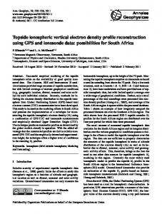
For the equilibrium internuclear distance 共Req = 1.423 a . u . , ␨ = 1.2, and Cion = 0.155兲, Fig. 1 displays, for several positions of the reference electron 1, the shape of the negative of nXC共rជ1 , rជ2兲 as a function of the position rជ2 when both rជ1 and rជ2 are located along the internuclear axis. Here, the origin is placed at the bond critical point 共BCP兲, which in this case is at the midpoint of the H–H bond. For rជ1 fixed at the BCP, the XC density spreads throughout the whole molecule, in similar fashion than the electronic density does. As the reference electron 1 moves into one of the basins, nXC tends, as expected, to be more localized within that basin,



J. Chem. Phys. 122, 214103 共2005兲

FIG. 1. Profile of −nXC for the H2 along its internuclear axis for three positions of the reference electron: at each of the hydrogen nuclei 共dashed and dotted lines兲 and at the BCP 共thin solid line兲. The origin is placed at the BCP, Req = 0.74 Å , ␨ = 1.2, and Cion = 0.155. Also, for comparison, the total density profile is displayed 共thick solid line兲.

A FIG. 2. Results of the function nXC along the H2 internuclear axis when the reference electron is placed at the BCP 共solid line兲 and at each of the hydrogen nuclei positions 共dashed and dotted lines兲. The positions along the internuclear axis are scaled with respect to the equilibrium internuclear distance 共Req = 0.74 Å兲.

i.e., increasing the exclusion of the other electron density from the volumes where it was initially concentrated. Our results also show that when the reference electron goes beyond any of the nuclear positions, the shape of the hole remains essentially constant 共rendering density distributions quite similar to those obtained for r1 = ± Req / 2兲. Additionally, the figure also indicates that, for all the studied cases, the XC density is not completely localized inside one of the basins, with a sizeable amount spreading out of it. In order to study the extent of the localization of the hole inside one of the basins, we have computed the function A ¯ 2nXC共1 , 2兲. Here, ␻ ¯ 2 denotes the nXC 共r1 , r2兲 ⬅ 兰r02dz2 兰⍀¯ Ad␻ coordinates of electron 2 perpendicular to the internuclear axis, r2 is the position of that electron along that axis, and nXC共1 , 2兲 is a short-hand notation for nXC共rជ1 , rជ2兲共which will be kept throughout this work兲. This function quantifies the amount of nXC共1 , 2兲 within the volume defined by the integration limits for a given reference electron position. We have numerically calculated this cylindrical coordinate integral within the A basin for several reference electron positions r1 placed along the internuclear axis. The results are presented in Fig. 2. First we notice that, for all the values of A r1 considered here, the negative of nXC 共r1 , r2兲 initially grows with r2; this is not surprising since more of the XC hole is included inside the A basin as r2 is shifted into it. Also it is observed that, for a fixed r2, when r1 moves into the basin, A 共r1 , r2兲 increases. This too is the negative of the function nXC an expected result, showing that the localization of the hole grows as the reference electron goes into the A basin. Additionally, for all the reference electron positions, it is observed that for r2 ⲏ 2Req the function becomes a plateau, indicating that at this position the whole XC density has been accounted for the integration and, at the same time, providing a measure of the outward extension of this density. The fact that this threshold position does not depend on r1 / Req seems

to indicate that, for this range of r2, the dominant factor in the localization of nXC is the interaction with the nucleus 共that clearly acts as an attractor for the density兲 regardless of the position of the other electron. It is interesting to notice that if the XC density were totally localized inside the basin, the value of the plateau would be −1. Nevertheless, for all the studied cases, values larger than this are obtained, meaning that the second electron is not totally excluded from ⍀A. Therefore, there is always a nonzero probability that both electrons are within the volume ⍀A at the same time, and consequently nXC共1 , 2兲 is shared between both atomic basins. Next, we study how the behavior of the XC density changes with the ionicity of the VB wave function. For several values of Cion, Fig. 3 shows the average of the XC density over the entire basin of one of the hydrogen atoms, A 具nXC 典共r1兲 ⬅ 兰⍀Adrជ2nXC共1 , 2兲, as a function of the position r1 of the reference electron 1, placed along the internuclear axis. Since we are dealing with a homonuclear molecule, the results for negative r1 are symmetrical to those displayed in A this figure and identical to −1 − 具nXC 典共r1兲. For a Cion chosen such that the wave function 共14兲 equals the Hartree–Fock 2 HF 共HF兲 wave function, i.e., Cion = 关2共1 + Sab 兲兴1/2 = 0.5877, it is A found that 具nXC典共r1兲 is constant and equal to 0.5. At this A 典 = 0.5, obtained point, let us recall that the value of 具nXC when the reference electron is at the position of the BCP, reflects the fact that the XC density is equally delocalized over both atomic basins. Therefore, the HF description corresponds to an approximation of the system with maximum HF electron delocalization. For Cion ⬍ Cion , when r1 moves into the A basin the XC density tends to be localized inside this basin 共increasing the localization as Cion decreases兲. Within the studied Cion range, two results deserve to be emphasized. A First, for r1 at or farther than the nuclear position, 具nXC 典 becomes independent of the reference electron position. Second, the XC density is not totally localized within the A

214103-5


214103-6

J. Chem. Phys. 122, 214103 共2005兲


A FIG. 3. Results of the average 具nXC 典 corresponding to the H2 molecule as a function of the reference electron position, when it is placed along the internuclear axis. The following values of the ionic coefficients are considered: 1 共thin solid line兲, 0.8 共dashed-double dotted line兲, 0.6 共dot-dashed line兲, 0.4 共dotted line兲, 0.2 共dashed line兲, 0 共thick solid line兲.

HF A basin 共i.e., 兩具nXC 典兩 ⬍ 1兲. On the other hand, for Cion ⬎ Cion it is A A found that 具nXC典 is an increasing function with 具nXC典 ⬎ −0.5. To understand this seemingly counterintuitive result, let us note that for this set of values of Cion the contribution to the density coming from the ionic species is, at least, comparable to that from the covalent one 关Eq. 共14兲兴. For the ionic contributions, both electrons are localized within one of the basins, while the other one is empty; therefore, when the ionicity grows, so it does the probability of finding both electrons within the same basin, which is reflected by the A 典. growth of the value of 具nXC

2. Variation with the internuclear distance

In order to study the effects of the variation of the internuclear distance on nXC共rជ1 , rជ2兲, we have evaluated the depenA 典 with the reference electron position for sevdence of 具nXC eral values of R. Before continuing, let us point out the well known fact30,35,36 that, at internuclear distances larger than the equilibrium one, the VB wave functions, as the one employed here, properly describe the qualitative behavior of the diatomic molecular systems studied in this work. Furthermore, due to the simplicity of the H2 system, for all these cases, the exponent constant and the ionicity parameters were adjusted variationally for each internuclear distance. The values employed in the calculations are reported in the caption of Fig. 4, which shows our results. Note that the ordinate is scaled with respect to the internuclear distances. First, notice that the behavior discussed regarding Figs. 1 and A 典共r1兲 keeps constant 3 remains valid for all R’s. That is, 具nXC after the reference electron reaches the nuclear position and, since for all these distances the ionization parameters are HF , the XC density is largely localized within smaller than Cion the reference electron basin. Also, as should be expected, the A 典 obtains its limiting nXC localization grows with R, and 具nXC

A FIG. 4. Results of the average 具nXC 典 corresponding to the H2 molecule as a function of the reference electron position, when it is placed along the internuclear axis, for several values of the internuclear distances. The positions along the internuclear axis are scaled with respect to the internuclear distance considered in each case. The values of Cion and ␨ corresponding to each R are, respectively, 0.135 and 1.307 共R = 0.53 Å, thick solid line兲, 0.149 and 1.249 共R = 0.64 Å, dot-dashed line兲, 0.155 and 1.200 共R = 0.74 Å, thin dotted line兲, 0.158 and 1.158 共R = 0.85 Å, dashed-double dotted line兲, 0.152 and 1.123 共R = 0.95 Å, thick dotted line兲, and 0.143 and 1.088 共R = 1.06 Å, thin solid line兲.

value at the dissociation limit. This is clear if we recall that as R increases, the overlap between the a and b orbitals diminishes, and so the electron delocalization throughout the molecule. Let us emphasize that this correct behavior cannot be reproduced within the HF approximation. In addition, within the studied range, it is observed that the saturation A value of 具nXC 典共defined as the constant value obtained after r1 reaches the nuclear position兲 changes linearly with respect to R. In order to understand qualitatively the behavior of the atomic localization index ␭共A兲 we present in Fig. 5 its variation as a function of Cion for three representative internuclear distances. The results show a near linear dependence, with the localization increasing with R in the limit of Cion → 0. For HF , it is obtained that all the Cion approximately equal to Cion ␭共A兲’s have a crossing point at a value close to 0.5. In agreement with the behavior displayed in Figs. 3 and 4, ␭共A兲 decreases with the ionicity. Additionally, the changes in ␭共A兲 are more noticeable as R grows.

B. The LiH case

In a similar fashion as for the H2, in this section we will discuss the properties of nXC共rជ1 , rជ2兲 for the LiH molecule. In Table I we present the values of the parameters ␨Li-1s , ␨Li-2s , ␨H-1s, and Cion for several internuclear distances R, estimated through the method explained in the preceding section.


214103-7

J. Chem. Phys. 122, 214103 共2005兲


FIG. 5. Variation of the atomic localization index of the H2 molecule as a function of the ionic coefficient, for the following internuclear distances: R = 0.53 Å 共dotted line兲, R = 0.75 Å 共dashed line兲, R = 1.06 Å 共solid line兲.

1. Equilibrium internuclear distance results

For several positions of the reference electron 1 along the internuclear axis, Fig. 6共a兲 exhibits the negative of the density of the XC hole as a function of the coordinate of electron 2, also placed along that axis. Note that the origin is fixed at the BCP. Even though the nuclear positions are not symmetrical with respect to the BCP, we may consider, as a guide, that the H nucleus is approximately at r1 / Req ⬇ −0.5, and the Li one at r1 / Req ⬇ 0.5. Again, if r1 is at the BCP, the XC density is spread over both atomic basins, as the electronic density. When the reference electron moves into one of the basins, nXC tends to become localized into it. The extension of this localization is much larger than that observed for the H2 case, and it is already observable for values of r1 as small as ±0.1Req. Moreover, the localization of the electron 1 共exclusion of other electrons兲 seems almost total when r1 is about the nuclear position, although it is more noticeable when r1 is at the Li position. In order to clarify the importance of each of the contributions to nXC, in Fig. 6共b兲 we show the XC density obtained from the parallel-spin component of the two-electron reduced density matrix and the one-electron density calculated from it, ␳␣␣+␤␤, i.e., TABLE I. Optimized values of the parameters ␨Li-1s , ␨Li-2s , ␨H-1s, and Cion, calculated through the method explained in the text, for several internuclear distances R. The values for the free H and Li atoms are also presented. Req = 1.63 Å is the equilibrium internuclear distance. R共Å兲

Cion

␨Li-1s

␨Li-2s

␨H-1s

1.0 1.3 Req 1.7 2.0 Atoms

0.680 0.622 0.597 0.561 0.522 ¯

2.740 2.731 2.711 2.711 2.710 2.700

0.642 0.642 0.642 0.643 0.645 0.650

1.290 1.280 1.279 1.264 1.223 1.000

FIG. 6. For the LiH molecule and in function of the electron coordinate along its internuclear axis 共scaled with respect to the equilibrium LiH inter␣␣+␤␤ nuclear distance兲 we present the following profiles: 共a兲 −nXC, 共b兲 −nXC , ␣␤+␤␣ and 共c兲 −nXC . In all the figures, the reference electron is placed at BCP 共dotted line兲, Li nuclear position 共thick solid line兲, and H nuclear position 共thin solid line兲. The origin is placed at the BCP, Req = 1.63 Å , ␨Li-1s = 2.711, ␨Li-2s = 0.642, ␨H-1s = 1.279, and Cion = 0.597.

␣␣+␤␤ 共1,2兲 = nXC

␣␣ ␣␣ 共1,2兲 + ⌫cov 共1,2兲 ⌫cov − ␳共2兲. ␣␣+␤␤ ␳ 共1兲

共28兲

This density may be largely associated with the exchange contribution to nXC. Let us mention that, for all values of r1 considered here, the integral of this density over the coordinate of electron 2 was found numerically to be −1. Figures 6共a兲 and 6共b兲 roughly show the same qualitative behavior; furthermore, the comparison of the density values for each case leads us to conclude that the exchange is, in fact, re-


214103-8

J. Chem. Phys. 122, 214103 共2005兲


sponsible for most of the exclusion of the other electrons. In particular, it is observed that when r1 is placed at the BCP, this contribution is virtually identical to the total XC hole. Nevertheless, some differences appear for the cases when the reference electron is placed at any of the nuclear positions. The excluded density decreases with respect to the one obtained from the total two-electron density. Thus, for r1 = RH, a small maximum, visible about the Li nuclear position, becomes more noticeable. While, if r1 = RLi, a new maximum appears about the hydrogen position. These results show that, if only the exchange contribution 共i.e., the Fermi hole兲 is considered, a lessening in the reference electron localization inside the corresponding basin is obtained. Therefore, a higher electronic delocalization may be predicted. To complement the discussion done so far, the results for the nXC density obtained from the antiparallel-spin component, ␣␤+␤␣ 共1,2兲 = nXC

␣␤ ␤␣ 共1,2兲 + ⌫cov 共1,2兲 ⌫cov − ␳共2兲, ␣␤+␤␣ ␳ 共1兲 ␣␤+␤␣

共29兲

is calculated from the are given in Fig. 6共c兲. Here, ␳ corresponding two-electron reduced density matrix. For this molecule, we have numerically checked that the integral of ␣␤+␤␣ nXC through the coordinate of electron 2 gives zero. From the figure we first observe that the values involved are ␣␣+␤␤ . When the reference electron is smaller than those of nXC at the BCP position, the values of this density are close to zero. On the other hand, if it is placed at the position of one of the nuclei, the exclusion from its basin reaches a maximum 共which is larger when r1 is at the Li position兲 driving, due to the Coulombic interaction, to an increase of the density of the other electrons inside the other nuclear basin. This behavior is shown as a maximum about the nuclear position where r1 is placed, and at a minimum about the other nuclear position. These minima approximately cancels the maximum of the Fermi hole, explaining the behavior of the total XC density of Fig. 6共a兲. Thus, these results indicate that indeed the contribution arising from the parallel-spin component of the two-electron reduced density matrix is the largest one. However, they also point to the fact that not including the antiparallel-spin component may lead to the missing of important qualitative features of the XC density. Before continuing, we would like to point out that the previous manner of estimating the exchange and correlation contributions to nXC is not the only one possible. The one chosen here satisfies the sum rules expected for the exchange and correlation holes, namely, 兰nX共1 , 2兲drជ2 = −1 and 兰nC共1 , 2兲drជ2 = 0 for any position of electron 1. Nevertheless, ␣␣+␤␤ ␣␤+␤␣ and nXC do not add to the total it is also clear that nXC nXC. We have tested another alternative definition that do satisfy this addition requirement, but do not comply with the previous sum rules, finding that even though the results differ quantitatively, they follow the same qualitative trends than the ones discussed for Fig. 6. Figure 7 shows the variation, in terms of the reference H 典共r1兲 for electron position along the internuclear axis, of 具nXC several values of Cion. The superindex denotes that the integration is performed through the H basin. The values of H 典 reflects that once the reference electron reaches posi具nXC

H FIG. 7. Variation of the average 具nXC 典 for the LiH molecule, for several values of the ionic coefficients, as a function of the reference electron position 共scaled with respect to the equilibrium LiH internuclear distance兲 when it is placed along the internuclear axis. The values of the ionic coefficients are 1 共dot-dashed line兲, 0.75 共thin solid line兲, 0.5 共dotted line兲, 0.25 共dashed line兲, and 0 共thick solid line兲. The origin is placed at the BCP, Req = 1.63 Å , ␨Li-1s = 2.711, ␨Li-2s = 0.642, ␨H-1s = 1.279.

tions r1 ⱗ −0.4Req, a sizeable exclusion of other electrons 共larger than 90%兲 is accomplished; therefore, a near complete localization of the reference electron over the H basin is achieved. This figure also shows how the localization is reduced as the ionic contribution to the total wave function gets larger. This could be understood if we recall that when Cion grows, the probability of having both electrons over the H basin increases, which should be reflected in a reduction of the exclusion of other electrons from this basin. In addition, our results show that for the cases where the reference electron is inside the Li basin, the electronic localization inside it grows rapidly. Note that this localization is practically total for r1 larger than 0.3Req, depending weakly on Cion and rendering slightly larger delocalization for larger Cion. 2. Variation with the internuclear distance

For several values of R, Fig. 8共a兲 exhibits the depenH 典 on r1, which is scaled with respect to the dence of 具nXC internuclear distances. For all cases, when r1 / R ⬍ −0.2 the observed behavior is qualitatively similar to that displayed in Fig. 7. Moreover, as expected, for r1 inside the H basin, the reference electron localization decreases when the internuclear distance shortens 共from ⬇100% for R ⬇ 1.2Req to 95% for R ⬇ 0.6Req, when r1 is nearby the H nuclear position兲. This could be understood by considering that for this distance, the overlap between the a and b orbitals grows, and hence, the electronic delocalization increases. Additionally, for r1 close to the H nuclear position, a very shallow minimum is observed. Since, for r1 = 0, the XC density is delocalized through the entire molecule, one would expect that H 典 would be nearly independent of the internuclear dis具nXC H 典 ⯝ 0.42 for all the tance. Indeed, this is the case, with 具nXC


214103-9


H FIG. 8. 共a兲 Average 具nXC 典 for the LiH molecule as a function of the reference electron position, for several values of the internuclear distance. H 共b兲 Same as 共a兲, but showing the antiparallel-spin average 具nXC,a 典. 共c兲 Same H 典. In all cases, the reference elecas 共a兲, but for the parallel-spin case 具nXC,p tron is placed along the internuclear axis and the values of the internuclear distances are R = 1 Å 共thin solid line兲, R = 1.3 Å 共dot-dashed line兲, R = Req 共dotted line兲, R = 1.7 Å 共dashed line兲, R = 2 Å 共thick solid line兲. The positions along the internuclear axis are given scaled with respect to the internuclear distance considered in each case. The values of the wave function parameters are given in Table I.

studied R, indicating that at this position of the reference electron, the exclusion is a little larger within the Li basin. For r1 / R ⬎ 0.1, the results for all these internuclear distances converge to approximately the same value. Finally, the figure shows that for r1 / R ⬎ 0.3, the results are practically independent of R, indicating that when the reference electron is placed this far inside the Li basin, its XC density is localized

J. Chem. Phys. 122, 214103 共2005兲

within this basin, not affecting the density distribution of the electrons on the H basin. This could be understood if we take into account that for this polarized system, most of the density on the Li basin is associated with core electrons of the Li, which are highly localized. In order to complement and better understand the previous information on the XC-density behavior, we have comH H puted the values of 具nXC 典 obtained from the parallel, 具nXC,p 典, H and antiparallel, 具nXC,a典, contributions to the two-electron and one-electron reduced density matrices 关Eqs. 共28兲 and 共29兲兴. The first gives a measure of the exchange contribution, while the second is associated to the Coulomb correlation contribution to nXC. In Fig. 8共b兲 we present the results for H 典. They indicate that the exclusion is largely due to the 具nXC,p exchange correlation. It is observed that, when the reference electron is placed well inside the H basin 共r1 / R ⬍ −0.4兲, the exclusion of the density of other same spin electrons does not show any large variation and displaying, as in the total density case, a very shallow minimum close to the H nuclear H 典 position. For the studied values of R, the results for 具nXC,p show that the exclusion is larger as R increases. As r1 approaches the BCP, the behavior is similar to the one described before. However, for this case a crossing point of the curves corresponding to different R’s is obtained when r1 ⯝ 0.1R. As the reference electron moves well inside into the Li basin 共r1 ⬎ 0.3R兲 a constant density exclusion on the H basin is obtained, being larger for shorter R. This indicates that at these internuclear distances the exclusion hole between same spin electrons is somewhat more delocalized. H 典 are displayed, it In Fig. 8共c兲, where the results for 具nXC,a H 典 reaches a is observed that, for r1 inside the H basin, 具nXC,a minimum, which is always located close to the H nuclear position. The results show that, for these cases, the Coulombic interaction between the reference electron and the other electrons excludes their density from the H basin. This repulsive interaction increases until the reference electron goes beyond the H nuclear position; past which the screening due to the nucleus becomes noticeable. In agreement to what was found for the parallel-spin contribution, the exclusion increases with R. Nevertheless, the dispersion range of the valH 典 is larger than 共⬃0.1兲, and its variation near the ues of 具nXC,a BCP is not as rapid as that obtained in that case. Additionally, here a well defined crossing point is observed at r1 ⯝ −0.05R, near the geometrical center of the molecule. Moreover, as the reference electron moves into the Li basin, H 典 gets positive values, being larger for larger internu具nXC,a clear distances. This density inclusion is also screened by the Li nucleus for r1 ⬎ 0.4R. This behavior is a consequence of the wave function ansatz, that only considers the contribution arising from the Li+H− resonance structure and privileges the location of two electrons within the H basin. This also points out the existence of a non-negligible Coulombic repulsion interaction between the reference and other electrons that tends to locate their density within the H basin. Thus, the set of results presented in Fig. 8 indicates that, even though most of exclusion is due to the parallel-spin contribution, the detailed behavior displayed by nXC is, in good measure, the consequence of the Coulombic correla-


214103-10

J. Chem. Phys. 122, 214103 共2005兲


eters related to the global behavior of both the charge and two-electron densities, as a measure of the bond character. This will be carried out in the next paper of this series. On the other hand, our results also establish that to obtain a correct qualitative behavior of nXC, it is necessary to go beyond the HF level of calculation. Thus, we have obtained that ionicities corresponding to HF wave functions lead to overestimations of the density delocalizations. We would like to emphasize that our goal in this paper was to study the trends in the behavior of these two limiting cases, which may be taken as references for later discussions of more complicated systems. Let us finish by stating that the results presented so far are intended to be semiqualitative at the best. Here, the valence-bond orbitals are considered as pure atomic Slater-type orbitals, the core orbitals are taken to be orthogonal to the valence ones and, for the LiH case, only one of the ionic contributions have been considered. These approximations should be improved in order to obtain more quantitative results, which will be approached in the next paper of this series. However, we think that the general trends obtained here will not be essentially affected by these improvements.

tion. Also, as expected for this kind of highly polarized systems, represented by the asymmetric ansatz wave function, the probability of having any pair of electrons with opposite spins, delocalized over both basins is small. IV. FINAL REMARKS

After finding analytical expressions for the first- and second-order reduced density matrices, we have obtained the XC density for two simple, but representative cases of molecular interactions. The starting point for this analysis was a valence-bond wave function,29,32–36 which can be considered as a special form of a multiconfigurational self-consistent field wave function,37 and is well suited to perform the kind of analysis presented here because it is capable to properly describe qualitatively the molecule for R ⬎ Req 共inclusion of enough of the nondynamical correlations兲. For several ionicities and internuclear distances, we have studied the behavior of the exchange-correlation hole, particularly its localization properties, as a function of the coordinates of an electron taken as reference. Additionally, in some cases, the results have been compared with those obtained from the HF level. A methodology is also proposed to analyze the exchange and correlation contributions to the total hole, which allows us to ponder their relative importance. The results show that the behavior of nXC clearly changes with the character of the bond, which here is given by the ansatz wave function and the values of its parameters. Therefore, it is indeed possible to obtain, in a practical manner, a good deal of information regarding the character of the bond interaction, which do not rely only on the value of the electronic density at a particular point, but instead consider the properties of the XC density as a whole. Thus, our results lead us to think that it is worthy to explore the use of param-

ACKNOWLEDGMENTS

This work was partially supported by grants of the Spanish Ministerio de Ciencia y Tecnología 共Grant No. BFM2001-1679-C093-03兲 and Ministerio de Educación y Ciencia 共Grant No. FIS-2004-05035-C03–03兲. R.A. is much obliged to the Spanish Ministerio de Educación, Cultura y Deporte for financial support during his sabbatical stay at the Universidad Nacional de Educación a Distancia. The authors acknowledge the continuous interest in this work of Dr. Pablo García-González.

APPENDIX: ANALYTICAL EXPRESSIONS FOR THE FIRST- AND SECOND-ORDER SPIN-FREE REDUCED DENSITY MATRICES OF H2 AND LiH

In what follows we present the expressions corresponding to the first- and second-order spin-free reduced density matrices used in this work. For the H2 molecule, the contributions are ⌫cov共1,2兲 =

␳cov共1兲 =

2 NH

2

2 共1 + Sab 兲 2 NH

2

2 共1 + Sab 兲

兵关a共1兲兴2关b共2兲兴2 + 关b共1兲兴2关a共2兲兴2 + 2a共1兲b共1兲a共2兲b共2兲其,

兵关a共1兲兴2 + 关b共1兲兴2 + 2Saba共1兲b共1兲其,

2 兵关a共1兲兴2关a共2兲兴2 + 关b共1兲兴2关b共2兲兴2 + 2a共1兲b共1兲a共2兲b共2兲其, ⌫ion共1,2兲 = 2NH 2

␳ion共1兲 = 2兵关a共1兲兴2 + 关b共1兲兴2 + 2Saba共1兲b共1兲其, ⌫res共1,2兲 =

␳res共1兲 =

2 4NH

兵关a共1兲兴 a共2兲b共2兲 + a共1兲b共1兲关b共2兲兴 2 冑2共1 + Sab 兲 2 NH

2

2

兵Sab关a共1兲兴 2 冑2共1 + Sab 兲 2

2

2

+ a共1兲b共1兲关a共2兲兴2 + 关b共1兲兴2a共2兲b共2兲其,

+ Sab关b共1兲兴2 + 2a共1兲b共1兲其.

For LiH, the results are Downloaded 04 Nov 2008 to 129.6.178.163. Redistribution subject to AIP license or copyright; see http://jcp.aip.org/jcp/copyright.jsp

214103-11

J. Chem. Phys. 122, 214103 共2005兲


␣␣ ␤␤ ⌫cov 共1,2兲 + ⌫cov 共1,2兲 =

2 NLiH 2 共1 + Sab 兲

„关␹共1兲兴2关a共2兲兴2 + 关␹共1兲兴2关b共2兲兴2 + 关a共1兲兴2关␹共2兲兴2 + 关b共1兲兴2关␹共2兲兴2 − 2关a共1兲␹共1兲a共2兲␹共2兲

+ b共1兲␹共1兲b共2兲␹共2兲兴 − 2Sab关a共1兲␹共1兲b共2兲␹共2兲 + b共1兲␹共1兲a共2兲␹共2兲兴 + 2Sab兵关␹共1兲兴2a共2兲b共2兲 + a共1兲b共1兲关␹共1兲兴2其…, ␣␤ ␤␣ 共1,2兲 + ⌫cov 共1,2兲 = ⌫cov


„2共1 + Sab兲兵关␹共1兲兴2关␹共2兲兴2 + 关␹共1兲兴2关a共2兲兴2 + 关␹共1兲兴2关b共2兲兴2 + 关a共1兲兴2␹共2兲2

+ 关b共1兲兴2关␹共2兲兴2 + 关a共1兲2兴关b共2兲兴2 + 关b共1兲兴2关a共2兲兴2 + 2a共1兲b共1兲a共2兲b共2兲其 + 2Sab兵关␹共1兲兴2a共2兲b共2兲 + a共1兲b共1兲关␹共2兲兴2其…,

␳cov共1兲 =


2 兵2共1 + Sab 兲关␹共1兲兴2 + 关a共1兲兴2 + 关b共1兲兴2 + 2Saba共1兲b共1兲其,

2 ␣␣ ␤␤ 共1,2兲 + ⌫ion 共1,2兲 = 2NLiH 兵关␹共1兲兴2关b共2兲兴2 + 关b共1兲兴2关␹共2兲兴2 − 2b共1兲␹共1兲b共2兲␹共2兲其, ⌫ion 2 ␣␤ ␤␣ ⌫ion 共1,2兲 + ⌫ion 共1,2兲 = 2NLiH 兵关␹共1兲兴2关␹共2兲兴2 + 关␹共1兲兴2关b共2兲兴2 + 关b共1兲兴2关␹共2兲兴2 + 关b共1兲兴2关b共2兲兴2其, 2 ␳ion共1兲 = 2NLiH 兵关␹共1兲兴2 + 关b共1兲兴2其,

␣␣ ␤␤ ⌫res 共1,2兲 + ⌫res 共1,2兲 =

2 2NLiH

„关␹共1兲兴 a共2兲b共2兲 + a共1兲b共1兲关␹共2兲兴 2 冑2共1 + Sab 兲 2

2

− 关a共1兲␹共1兲b共2兲␹共2兲 + b共1兲␹共1兲a共2兲␹共2兲兴

+ Sab兵关␹共1兲兴2关b共2兲兴2 + 关b共1兲兴2关␹共2兲兴2 − 2b共1兲␹共1兲b共2兲␹共2兲其…, ␣␤ ␣␤ 共1,2兲 + ⌫res 共1,2兲 = ⌫res

2 2NLiH

„关␹共1兲兴 a共2兲b共2兲 + a共1兲b共1兲关␹共2兲兴 2 冑2共1 + Sab 兲 2

2

+ 关b共1兲兴2a共2兲b共2兲␹共2兲 + a共1兲b共1兲关b共2兲兴2

+ Sab兵关␹共1兲兴2关b共2兲兴2 + 关b共1兲兴2关␹共2兲兴2 + 2关␹共1兲兴2关␹共2兲兴2其…,

␳res共1兲 =

2 2NLiH

„a共1兲b共1兲 + 2Sab兵关␹共1兲兴 2 冑2共1 + Sab 兲

2

+ 关b共1兲兴2其….

P. Hohenberg and W. Kohn, Phys. Rev. 136, B864 共1964兲. W. Kohn and L. J. Sham, Phys. Rev. 140, A1133 共1965兲. 3 R. S. Mulliken, J. Chem. Phys. 23, 1833 共1955兲. 4 R. F. W. Bader, Atoms in Molecules: A Quantum Theory 共Oxford University Press, Oxford, 1990兲. 5 R. F. W. Bader, Chem. Rev. 共Washington, D.C.兲 91, 893 共1991兲. 6 A. D. Becke and K. E. Edgecombe, J. Chem. Phys. 92, 5397 共1990兲. 7 A. D. Becke, Int. J. Quantum Chem. 23, 1925 共1983兲. 8 B. Silvi and A. Savin, Nature 共London兲 371, 683 共1994兲. 9 A. E. Reed, L. A. Curtis, and F. Weinhold, Chem. Rev. 共Washington, D.C.兲 88, 899 共1988兲. 10 I. Mayer, Int. J. Quantum Chem. 24, 477 共1986兲. 11 I. Mayer, Chem. Phys. Lett. 97, 270 共1983兲. 12 C. G. Zhan, J. Mol. Struct.: THEOCHEM 101, 193 共1993兲. 13 G. N. Lewis, J. Am. Chem. Soc. 38, 762 共1916兲. 14 L. Pauling, The Nature of the Chemical Bond 共Cornell University Press, Ithaca, NY, 1939兲. 15 P.-O. Löwdin, Phys. Rev. 97, 1474 共1955兲; 97, 1490 共1955兲; 97, 1509 共1955兲. 16 R. McWeeny, Rev. Mod. Phys. 32, 335 共1960兲. 17 E. R. Davidson, Reduced Density Matrices in Quantum Chemistry 共Academic, New York, 1976兲. 18 R. G. Parr and W. Yang, Density Functional Theory of Atoms and Molecules 共Oxford University Press, Oxford, 1989兲. 19 J. P. Perdew and S. Kurth, in A Primer in Density Functional Theory, edited by C. Fiolhais, F. Nogueira, and M. Marques 共Springer, Berlin, 2002兲. 20 J. P. Perdew and A. Zunger, Phys. Rev. B 23, 5048 共1981兲. 21 R. F. W. Bader, S. Johnson, T.-H. Tang, and P. L. A. Popelier, J. Phys. Chem. 100, 15398 共1996兲. 1 2

22

R. F. W. Bader, A. Streitweiser, A. Neuhaus, K. E. Laidig, and P. Speers, J. Am. Chem. Soc. 118, 4959 共1996兲. 23 X. Fraderas, M. A. Austen, and R. F. W. Bader, J. Phys. Chem. 103, 304 共1999兲. 24 X. Fraderas, J. Poater, S. Simon, M. Duran, and M. Solà, Theor. Chim. Acta 108, 214 共2002兲. 25 P. C. Hiberty and D. L. Cooper, J. Mol. Struct.: THEOCHEM 169, 437 共1988兲. 26 G. Sini, P. Maitre, P. C. Hiberty, and S. Shaik, J. Mol. Struct.: THEOCHEM 229, 163 共1991兲. 27 S. Shaik, P. Maitre, G. Sini, and P. C. Hiberty, J. Am. Chem. Soc. 114, 7861 共1992兲. 28 L. Rincón and R. Almeida, J. Phys. Chem. A 102, 9244 共1998兲. 29 R. S. Mulliken, C. A. Rieke, D. Orloff, and H. Orloff, J. Chem. Phys. 17, 1248 共1949兲. 30 F. E. Penotti, Int. J. Quantum Chem. 59, 349 共1996兲. 31 A. D. McLean and G. S. Chandler, J. Chem. Phys. 72, 5639 共1980兲. 32 F. W. Bobrowicz and W. A. Goddard, in Method of Electronic Structure Theory, edited by H. F. Schaefer 共Plenum, New York, 1977兲. 33 M. J. Frisch, G. W. Trucks, H. B. Schlegel et al., GAUSSIAN 98, Revision A. 6, Gaussian, Inc., Pittsburgh, PA, 1998. 34 W. H. Press, B. P. Flanery, S. A. Teukolsky, and W. T. Vetterling, Numerical Recipes in Fortran 共Cambridge University Press, Cambridge, 1992兲. 35 D. L. Cooper, J. Gerratt, and M. Raimondi, Adv. Chem. Phys. 69, 319 共1987兲. 36 D. L. Cooper, J. Gerratt, and M. Raimondi, Chem. Rev. 共Washington, D.C.兲 85, 92 共1991兲. 37 A. Szabo and N. S. Ostlund, Modern Quantum Chemistry 共Dover, New York, 1989兲.
