electronic reprint Journal of
Applied Crystallography ISSN 0021-8898
Editor: Anke R. Pyzalla
Irena: tool suite for modeling and analysis of small-angle scattering Jan Ilavsky and Peter R. Jemian
J. Appl. Cryst. (2009). 42, 347–353
c International Union of Crystallography Copyright !
Author(s) of this paper may load this reprint on their own web site or institutional repository provided that this cover page is retained. Republication of this article or its storage in electronic databases other than as specified above is not permitted without prior permission in writing from the IUCr. For further information see http://journals.iucr.org/services/authorrights.html
Many research topics in condensed matter research, materials science and the life sciences make use of crystallographic methods to study crystalline and non-crystalline matter with neutrons, X-rays and electrons. Articles published in the Journal of Applied Crystallography focus on these methods and their use in identifying structural and diffusioncontrolled phase transformations, structure–property relationships, structural changes of defects, interfaces and surfaces, etc. Developments of instrumentation and crystallographic apparatus, theory and interpretation, numerical analysis and other related subjects are also covered. The journal is the primary place where crystallographic computer program information is published.
Crystallography Journals Online is available from journals.iucr.org J. Appl. Cryst. (2009). 42, 347–353
Ilavsky and Jemian · Irena
computer programs Journal of
Applied Crystallography
Irena: tool suite for modeling and analysis of smallangle scattering
ISSN 0021-8898
Jan Ilavsky* and Peter R. Jemian Received 25 September 2008 Accepted 16 January 2009
# 2009 International Union of Crystallography Printed in Singapore – all rights reserved
Advanced Photon Source, Argonne National Laboratory, 9700 S Cass Avenue, Argonne, IL, USA. Correspondence e-mail:
[email protected]
Irena, a tool suite for analysis of both X-ray and neutron small-angle scattering (SAS) data within the commercial Igor Pro application, brings together a comprehensive suite of tools useful for investigations in materials science, physics, chemistry, polymer science and other fields. In addition to Guinier and Porod fits, the suite combines a variety of advanced SAS data evaluation tools for the modeling of size distribution in the dilute limit using maximum entropy and other methods, dilute limit small-angle scattering from multiple noninteracting populations of scatterers, the pair-distance distribution function, a unified fit, the Debye–Bueche model, the reflectivity (X-ray and neutron) using Parratt’s formalism, and small-angle diffraction. There are also a number of support tools, such as a data import/export tool supporting a broad sampling of common data formats, a data modification tool, a presentation-quality graphics tool optimized for small-angle scattering data, and a neutron and X-ray scattering contrast calculator. These tools are brought together into one suite with consistent interfaces and functionality. The suite allows robust automated note recording and saving of parameters during export.
1. Introduction Small-angle scattering (SAS) techniques using neutrons or X-rays are widely used for investigations in materials science, chemistry, polymer physics and other areas of science where nanoscale characterization is necessary. Continuing developments in theory and increasingly complex analytical models are trying to satisfy the needs of advanced materials science, chemistry, biology and a broad range of other scientific disciplines in which SAS investigations are undertaken (Pedersen, 1997). At the same time a variety of factors, such as advances in instrumentation and radiation sources, and improvements in detectors, have led to dramatic increases in data acquisition rates. Software tools for the analysis of collected data must be improved so that they do not become a factor limiting the progress of scientific programs. SAS data processing can be subdivided into two steps – data reduction and data analysis – which, while sometimes intertwined, are often separable. Reduction of SAS data is often closely related to the instrument (hardware) design and setup, as evidenced by the development of a number of instrument-specific data reduction packages: e.g. for the NIST SANS instruments (Kline, 2006), ESRF ID2 SAXS (Boesecke, 2007), APS ChemMatCARS SAXS (Cookson et al., 2006) and APS USAXS (Indra; Ilavsky et al., 2009, 2002). A few data packages such as Fit2D (Hammersley, 1997), Nika (Ilavsky, 2008) and Datasqueeze (Heiney, 2005) attempt to provide generic tools. The analysis and modeling of SAS data are often independent of the particulars of any instrument, assuming that instrumental effects such as (angle or wavelength) smearing can be modeled or corrected during data reduction. A significant community of open source software packages for the analysis of SAS are currently available for the Igor Pro commercial scientific analysis application (Wavemetrics, 2008): the NIST analysis tools (Kline, 2006), Motofit (reflectivity) J. Appl. Cryst. (2009). 42, 347–353
(Nelson, 2006) and the SAS analysis tool suite Irena (this work) to name just a few. The source code for each of these is distributed as text files. The distribution of the source code is significant since it is therefore available for scrutiny.
2. Basic information The Irena SAS suite contains tools for analysis of small-angle scattering applicable to investigations in materials science, chemistry, polymer science and a number of other fields where SAS is used. Its development started around the year 2000 in order to satisfy the needs of users of the Advanced Photon Source ultra-small-angle X-ray scattering (USAXS) facility (Ilavsky et al., 2009, 2002; Long et al., 1991). This USAXS facility supports a wide range of programs in materials science – metals, ceramics, polymers and combinations, as well as solutions, gels and other soft materials. A single flexible analysis tool suite was needed to support such a wide range of problems. The tool suite grew to include contributions that had been developed previously by others and for other facilities. The names of these contributors and references to appropriate publications are included in the description of each tool in the included manual. During 2008, Irena averaged about 30–45 downloads per month, and it currently has a mailing list of about 55 registered users. Users from the US (Allen, 2005; Allen et al., 2007; Braun, Ilavsky, Dunn et al., 2005; Braun, Ilavsky, Seifert & Jemian, 2005; Justice et al., 2007; Kammler et al., 2004; Kulkarni et al., 2006, 2004; Levine et al., 2007; Schaefer et al., 2003; Schaefer & Justice, 2007; Tirumala et al., 2006) and the rest of the world (Woodward et al., 2007; Paskevicius & Buckley, 2006) have used it for publication quality work.
electronic reprint
doi:10.1107/S0021889809002222
347
computer programs 2.1. Documentation
Irena is accompanied by a user manual, synchronously updated with the code. This manual describes the theory underlying each tool, with references where available, and guides the user through an example use of the tool, explaining the function of every switch/input variable. It assumes the reader has a basic proficiency in small-angle scattering. The functionality of selected internal libraries that may be useful to other programmers (data selection tool, form factor library and structure factor library) is described in a separate document as well as in comments within the source code.
Many tools can also generate model SAS data, i.e. without the presence of input data, and can generate arithmetic or geometric progressions of Q values with user-defined parameters. The primary input and output data format is columnar ASCII, one data set per file, or the canSAS1d XML (also known as SASXML) data format (http://www.smallangles.net/wgwiki/index.php/ cansas1d_documentation). Any extra tags or comments can be included in the wavenotes (see x2.3) of imported data as metadata for future use. Data can also come from the USAXS data reduction package Indra (Ilavsky et al., 2002), the area-detector data reduction package Nika (Ilavsky, 2008) and from some other Igor-based data reduction packages (SANS instruments at HFIR, ORNL). 2.3. Record keeping
2.2. Data
Fully reduced and calibrated one-dimensional SAS data sets are the expected input to Irena, where intensity is a function of the ˚ !1). While intensity units on an absolute scale scattering vector Q (A (cm!1) are preferred, this is not a strict requirement. Size dimensions of scatterers are consistently represented in a˚ngstro¨ms. Many of the tools in the suite rely on the presence of uncertainty estimates (also termed ‘errors’) for intensities. These should be given as one standard deviation. All Irena tools assume perfect Q resolution, i.e. no Q-resolution smearing is performed. This perfect Q resolution is a very good approximation for USAXS instruments (where the Q resolution of all ˚ !1 or better) and is often a good approximation data is "1 # 10!4 A for SAXS or SANS data from samples where the scattered intensity changes slowly within the instrument Q resolution. For users of slit-smeared instruments, Irena tools (except for the reflectivity tool) have the capability to optionally slit smear the model data and therefore can be applied directly to slit-smeared data (with finite slit length smearing) without prior desmearing of the data. When needed, a desmearing tool is available, as discussed later in this article.
Each of the analysis tools has a relatively large number of associated parameters that users may wish to record. To assist users with data handling and management, Irena has a built-in automatic record keeping system, comprising a method of storing final results and tools to search through the stored results and generate user-friendly outputs. All tools record important parameters in an internal notebook before and after each fitting or optimization run. These parameters are stored and can be searched later as necessary. Irena stores metadata for each data set using an internal capability of the application known as the wavenote. Analysis parameters are recorded in these wavenotes as a text list of keyword ¼ value; pairs with meaningful keywords. This enables easy identification of the results and associated parameters, especially when using the Irena tool provided. 2.4. Optimization methods
Except for the size distribution and the pair-distance distribution tools (see xx3.2 and 3.7), Irena tools by default use the Levenberg– Marquardt (L–M) least-squares method provided by the application. Occasionally, the L–M method may not converge upon the global minimum of the fitting function and thus may not achieve the best fit possible. The usual way to verify the integrity of the solution is to run an optimization multiple times with slightly different starting conditions. Furthermore, the Modeling I, Modeling II and reflectivity tools take advantage of genetic optimization (Wormington et al., 1999), a Monte Carlo method originally developed for use in the analysis of X-ray reflectivity data. The software for this method has been provided by Nelson (2006), as part of his reflectivity modeling package Motofit. While this method is significantly slower than regular least-squares fitting it sometimes achieves superior results. 2.5. Graphical user interface
For a tool suite of such complexity as Irena, it is most important to help researchers preserve their focus on the science at hand by maintaining consistency in the graphical user interface (GUI). Typical Irena screens are presented in Figs. 1 and 2. The GUI layout is organized in the order of use – the user should start with controls at the top of the panel, continue downward and end with controls at the bottom of the panel. The controls vary depending on the needs of each tool. Online help is provided for each control element through the built-in help system of the application. Figure 1
2.6. Details on code behavior
Typical example (from unified fit) of the GUI and controls used in most Irena tools. The GUI is divided into a top section with input data selection, a middle section with model controls, and a bottom section with fitting and output controls.
All Irena tools have been designed to operate concurrently, allowing scientists to compare analytical approaches from different
348
Ilavsky and Jemian
%
Irena
electronic reprint
J. Appl. Cryst. (2009). 42, 347–353
computer programs tools. Parameters for each tool are initialized from Irena defaults when the tool is first used. User selections are saved as defaults for the next time the tool is used. The user selections are also recorded as metadata in the wavenotes or saved results. When data are loaded for analysis into a tool, its data folder is scanned for saved results from a previous analysis using this tool. If one or more results are found, the user is presented with a dialog with options to recover the parameter values from any of the existing results (using the metadata) or to keep the present default parameter values.
3. Modeling and analysis tools
Table 1 Summary of features of the Modeling I and Modeling II tools. Feature
Modeling I
Modeling II
Number of populations Input data sets Contrast for each population Form factors Structure factor
Up to 5 1 1
Up to 6 Up to 10 Up to 10 – different for each data set Choice of 12‡ Dilute limit or choice of 4‡
Least-squares fitting Genetic optimization Size distribution binning
Choice of 12† Dilute limit or ‘interferences’‡ Yes Yes Automatic
† Some parameters cannot be fitted.
Many different tools comprise the Irena tool suite, each added and enriched in response to the needs of the user community. While a brief explanation of each tool is provided here, the reader is directed to the user manual and literature citations for further explanation. 3.1. Non-interacting dilute systems modeling
Two versions of this tool are currently available. Development of the older, simpler version (Modeling I) has been frozen, but since this is one of the most popular Irena tools, it is being maintained. Modeling II was developed to provide additional capabilities. Both tools share the same philosophy and mathematics. They share a library of form factors, and Modeling II uses also a library of structure factors. Using these libraries enables simple extension of capabilities when needed. Table 1 shows a comparison of the capabilities of Modeling I and Modeling II. 3.1.1. Model. Both Modeling I and Modeling II calculate the intensity of small-angle scattering from particles in multiple populations of scatterers (Guinier & Fournet, 1955; Porod, 1982). While the populations are described in terms of their number distribution, N(D), it has been found that greater numerical stability can be achieved if the formula for intensity is expressed in terms of volume
Yes Yes Automatic, semi-automatic, user-defined
‡ Parameters can be fitted.
fraction distribution of scatterers, f(D). Replacing the integration over a continuous size distribution with a summation over a discrete size histogram, the formula in the code is P P IðQÞ ¼ j!!k j2 Sk ðQÞ jFk ðQ; Dik Þj2 Vk ðDik Þ fk ðDik Þ !Dik ; ð1Þ k
ik
where the subscript i includes all bins in the size distribution and !Di is the width of bin i. Subscript k represents different populations; each population has its own binning index ik. D is the dimension of the particle (e.g. radius for spheres), |!!|2 is the scattering contrast, S(Q) is the structure factor, F(Q, D) is the scattering form factor and V(D) is the particle volume. f(D) is the volume size distribution, which is related to the number size distribution N(D) through ð2Þ
f ðDÞ ¼ VðDÞ NðDÞ ¼ VðDÞ NT "ðDÞ;
where NT is the total number of scattering particles, V(D) is the volume of the particle and "(D) is the probability of occurrence of a scatterer of size D. Four different size distributions are available – Gauss (normal), lognormal, Lifshitz–Slyozov–Wagner (LSW; Lifschitz & Slyozov, 1961; Wagner, 1961) and power law (useful when modeling fractal systems). These size distributions can be used to model either volume distributions f(D) or number distributions N(D). For both tools, all populations must share the type (volume or number) of distribution modeled, but this choice is individual for each tool. 3.1.2. Natural binning. The theoretical ranges of the various size distributions in Irena can vary. For example, the lognormal distribution ranges from 1/1 to 1, while the LSW distribution needs only to extend as high as 1.5 times the normalized particle radius (Lifschitz & Slyozov, 1961; Wagner, 1961). Numerical calculations, however, require limits on the range of dimensions (minimum and maximum dimensions considered). Natural binning for the size distributions used by Irena makes this easy and robust for users. This method results in a nonlinear stepping in dimension and uses two user parameters – number of bins, Nb, and fractional volume to be neglected, 2VN. Figure 2 Fig. 3 indicates graphically how the binning Example of the Modeling II tool GUI. The left panel has controls for both the input data and the model. On the is obtained for an arbitrary distribution: a right, the top graph shows the input data and scattering calculated from the working model size distribution, while the bottom graph shows the working model size distribution. cumulative distribution is created by J. Appl. Cryst. (2009). 42, 347–353
electronic reprint
Ilavsky and Jemian
%
Irena
349
computer programs numerical integration of the given distribution. The center of the first bin (smallest dimension) is found as that value for which the cumulative function equals VN, and the center of the last bin (largest dimension) is the value for which the cumulative function equals (1 ! VN). The intervening bins are found by selecting associated dimensions at regular increments of the cumulative distribution ! ¼ ð1 ! 2VN Þ=ðNb ! 1Þ;
ð3Þ
where Nb is the user-defined number of bins, as described in Fig. 3. These dimensions become centers of the bins. The bin edges are found as midpoints between two neighboring bin centers. The first and last bin widths are made symmetrical around their centers. This guarantees that only a volume less than 2VN is neglected (not modeled) in calculations. This method can result in bins with D values that are too small (or even negative) to be physically meaningful. It is not physically meaningful to interpret scatterer sizes smaller than "0.5 nm from SAS data. Therefore, during intensity calculations, bins with dimension smaller than 0.4 nm are discarded. This may result in artifacts and should be considered by users. 3.1.3. Form factors available. Both modeling tools and the size distribution tool share a common library of form factors. All form factor formulae are explained in the documentation included with Irena, including Igor code, references and graphs. The form factors currently included can be divided into two types: (1) exact analytical formulae (e.g. Shull & Roess, 1947; Roess & Shull, 1947; Kostorz, 1979; Porod, 1982; Pedersen, 2000), which can often be slow to evaluate, and (2) approximate but much faster evaluating functions, such as algebraic formulae (Allen et al., 1993) or formulae based on the unified fit (Beaucage, 1995). Users can provide additional form factors by providing Igor functions that calculate the form factor and the particle volume. 3.1.4. Structure factor library. By default, the modeling is performed in the dilute limit; however, the structure factor can be modeled when necessary. Both Modeling I and the unified fit tools (see later) include a simple model of interparticle interference (from Beaucage et al., 1995), SðQÞ ¼
1 ; 1 þ 3"½sinðQ#Þ ! Q# cosðQ#Þ*=ðQ#Þ3
ð4Þ
which approximates a hard sphere model but with different definitions for the parameters " (packing factor) and # (correlation distance). No further corrections (Hayter & Penfold, 1983; Kotlarchyk & Chen, 1983) are currently implemented.
Figure 3 Demonstration of natural binning selection for an arbitrary size distribution.
350
Ilavsky and Jemian
%
Irena
Modeling II extends the capabilities by including additional structure factors, the code for which is adopted from the NIST Igor package (Kline, 2006): Percus–Yevick model hard spheres (Percus & Yevick, 1958; Thiele, 1963; Wertheim, 1963), square well (Sharma & Sharma, 1977), sticky hard spheres (Kline & Kaler, 1998) and Hayter–Penfold MSA (Hayter & Penfold, 1981).
3.2. Size distribution tool
The Irena size distribution tool provides a common interface to three methods: the maximum entropy (MaxEnt), regularization (maximizes smoothness) and total non-negative least-squares methods. The tool seeks a solution for f(D) from equation (1) in the dilute limit where the approximation S(Q) = 1 is acceptable and all populations in equation (1) are assumed to be isomorphous so that the subscript k may be discarded. Equation (1) is ill-conditioned in that F(Q, D) ranges over many orders of magnitude. In this tool the method of solution for f(D) must be constrained to avoid noise or singularities in the solution. The size distribution here is not restricted to a particular functional form, such as Gaussian or lognormal, as in Modeling I and II. The Irena size distribution tools provide results presented as both N(D) and f(D). Internally, the size distribution tools use f(D). 3.2.1. Maximum entropy. The maximum entropy method for SAS data analysis was developed by Potton et al. (1983, 1988a,b) and further advanced by Jemian et al. (1991). It relies on the maximum entropy engine of Skilling and Bryan (Bryan, 1990; Bryan & Skilling, 1980, 1986; Skilling & Bryan, 1984). Details of the MaxEnt method are not repeated here as they are beyond the scope of this article. 3.2.2. Regularization. The regularization method was developed in response to perceived shortcomings in the MaxEnt approach, resulting occasionally in a not credible oscillatory structure in the resultant size distributions. Therefore an alternative method of constraining the smoothness of the solution for f(D) was developed, called regularization. Regularization thus selects the smoothest solution subject to fitting the measured data. In both the MaxEnt and the regularization methods, the goodness of fit criterion $2 (sum of squared standardized residuals) must be close to the number of measured data points used in the analysis, subject to an additional constraint of maximizing the entropy or smoothness of the solution. This imposes a high standard for the reported errors on the scattering intensity. The reported errors are expected to be proper 1% standard deviation error estimates (exact knowledge of the experimental errors would vastly simplify the solution). If errors are not correct, it is likely that artifacts in the derived size distribution will result. Often it is necessary to scale the reported errors by a factor to achieve convergence of the MaxEnt method. 3.2.3. Total non-negative least-squares method. The total nonnegative least-squares (TNNLS) method implements the work of Merritt and Zhang (Merritt & Zhang, 2004; Zhang, 2004). Contrary to the MaxEnt and regularization methods, the uncertainties are used only to identify a sufficiently good solution, i.e. to calculate $2. To improve convergence when the scattering data span large intensity and Q ranges, an optional ‘Q-weighting’ of intensity is implemented. If selected, both the data intensities and the model are multiplied by QN, where N is any integer from 0 to 4. This was found to change the conditioning of the scattering equation and often results in more credible fits.
electronic reprint
J. Appl. Cryst. (2009). 42, 347–353
computer programs 3.3. Unified fit tool
The unified fit tool is based on the unified exponential/power-law approach to small-angle scattering and the Igor code developed by Beaucage and co-workers (Beaucage, 1995, 1996, 2004; Beaucage et al., 1997, 1995), which models SAS with ‘structural levels’. Scattering from each level is considered to be composed of a Guinier exponential form and a structurally limited power law. The code handles various data for which development of an exact scattering model is difficult or impossible. The calculations either are performed in the dilute limit or can be combined with a structure factor using ‘interferences’ (see above). The tool provides for as many as five independent levels (n = 5), including structure factor: ! n P IðqÞ ¼ FB þ Si ðQÞ Gi expð!Q2 R2gi =3Þ þ Bi expð!Q2 R2gcfi =3Þ n
i¼1
# ½erfðQRgi =61=2 Þ*3 =Q
oPi " ;
ð5Þ
where FB is an optional flat background, i represents the structural levels, and, for each structural level i, Gi is the exponential prefactor, Rgi is the radius of gyration and Bi is a constant prefactor specific to the type of power-law scattering, Pi. For Porod’s law, P = 4, Bi is the Porod constant and is related to the specific surface area of the scatterers of that level. Furthermore, Rgcfi is the high-Q power-law cut-off radius, important for multiple structural levels (Beaucage, 1995, 1996). Further details of the theory are beyond the scope of this paper. The unified fit tool uses the Levenberg–Marquardt least-squares fitting from the application to optimize parameters. 3.4. Debye–Bueche tool
The Debye–Bueche tool was developed for modeling structural inhomogeneities in gels (Tirumala et al., 2006). The intensity is modeled using the Debye–Bueche (Debye & Bueche, 1949) formula, IðQÞ ¼ 4&K"2 CL2 =ð1 þ Q2 CL2 Þ2 ;
ð6Þ
2 !4
where K ¼ 8& ' . The main model parameters are " (scaling factor) and CL (correlation length). To accommodate samples that exhibit power-law scattering at low Q, the model also incorporates power-law scattering with a prefactor B and power-law slope P. In addition, the model includes a flat background FB, which can be fitted at the same time using leastsquares. Therefore the final formula, fitted by least squares, is IðQÞ ¼ FB þ BQ!P þ 4&K"2 CL2 =ð1 þ Q2 CL2 Þ2 :
ð7Þ
3.5. Fractals model tool
A number of scattering systems can be described as surface or volume fractals (Beaucage, 2004, 1996; Kammler et al., 2005). Usually fractal systems are modeled with the unified fit tool and described mostly by their fractal dimensions (Beaucage, 2004, 1995); however, a more exact theory, used in the fractals tool, is currently available and in some cases applicable (Allen et al., 2007). The scattering systems can be as composed of up to two surface and two volume fractals. The model predicts Q!Dv scattering (i.e. between Q!1 and Q!3) for mass or volume fractals and Q!(6!Ds) scattering (i.e. between Q!3 and Q!4) for surface fractals. This model requires scattering data over an extended Q and intensity range, such as one can obtain from a combination of measurements on multiple instruments, measurements with multiple sample-to-detector distances, or measurements using a USAXS or USANS instrument. The formula used by the J. Appl. Cryst. (2009). 42, 347–353
fractals tool is quite complex and the description, provided in the Irena documentation, is beyond the scope of this paper. 3.6. Reflectivity tool
The reflectivity tool can model and fit X-ray and neutron reflectivity for up to eight layers using either the recursive code of Parratt (1954) or the Abeles matrix method (Nelson, 2006), both with extension for surface roughness. The code itself was implemented previously by Nelson (2006) and is used also in Irena. For a full explanation of the reflectivity methods used in these calculations, please see Nelson (2006), and references cited therein. For more complex analyses (e.g. a slab model with more than eight layers or a need for interparameter constraints), the reader is referred to Motofit, available for free download (http://motofit.sourceforge.net/) under GNU license. The reflectivity tool can use instrument Q-resolution data, either as provided in a list or calculated from instrument parameters. 3.7. Pair-distance distribution function
In terms of the pair-distance distribution function (0 ðrÞ (Kostorz, 1979; Guinier & Fournet, 1955; Glatter & Kratky, 1982), IðQÞ ¼ ð!!Þ2 V ¼ ð!!Þ2 V
RD 0
4&r2 dr (0 ðrÞ sinðQrÞ=ðQrÞ
D P 0
4&r2 !r (0 ðrÞ sinðQrÞ=ðQrÞ:
ð8Þ
For the purpose of analysis in this tool, ð!!Þ2 V = 1. Therefore, the results are only relative, as the contrast and volume of scatterers are not considered. This tool uses two analysis methods – regularization, explained above, and the indirect Fourier transformation method of Moore (1980). Both result in (0 ðrÞ, but the indirect Fourier transformation method can also optimize the maximum dimension Dmax and the flat background, which the regularization method cannot. 3.8. Small-angle diffraction
The small-angle diffraction tool models data composed of smallangle scattering (modeled by a single unified level), flat background and up to six diffraction peaks. The diffraction peak "(Q) profiles available are Gaussian, modified Gaussian, Lorentzian, pseudoVoigt, Pearson-VII and Gumbel shapes (NIST/SEMATECH e-Handbook of Statistical Methods, http://www.itl.nist.gov/div898/ handbook/). Each of these peak profiles has a scaling factor and up to three shape parameters, which can all be optimized using leastsquares fitting. The formulae of these shapes are given in the manual. It is possible either to fit the positions of the peaks independently or to create fixed relationships among the positions of the peaks, as appropriate for a given structure, and optimize the positions together. Selected peak position ratios for ten structures are predefined in the tool (Hadjichristidis et al., 2003). Two options for calculating peak intensity are implemented: P ð9aÞ IðQÞ ¼ IUnified ðQÞ þ FB þ IUnified ðQÞKi "i ðQÞ i
or
IðQÞ ¼ IUnified ðQÞ þ FB þ
P
peaks
Ki "i ðQÞ;
ð9bÞ
where Ki is the scaling factor for each diffraction peak. The peak parameters provided as results to users are the numerically calculated values for Ki"i(Q) in both cases.
electronic reprint
Ilavsky and Jemian
%
Irena
351
computer programs 3.9. Scripting tool
The scripting tool is designed to provide the capability to run either the size distribution or the unified fit tool on a large number of data sets in a non-interactive mode. It provides a GUI to select multiple data sets and then controls the GUI of the main tool.
4. Support tools A number of tasks not directly related to data analysis need to be routinely performed by users, e.g. data import or export and modification. Irena contains tools that cover most of the common needs of users in this area. 4.1. Data import and export tools
These tools help users to import ASCII and canSAS1d XML files and export ASCII files. The data import tool enables users to import one or more data sets into the current Igor experiment while optionally performing some basic modifications of the data: ˚ !1, scaling intensity by a scaling converting Q values from nm!1 to A factor and generating errors (percent errors or square-root errors) when user errors are not provided. The data export tool helps users export various types of data (measured data or results of modeling) from the current Igor experiment. 4.2. Data manipulation tool
Using this tool, a user can trim and/or scale up to two (xy, and error if available) data sets. Furthermore, the user can perform a number of operations on two data sets: e.g. merge, sum, subtract and divide. Data can also be re-binned using the x values of a second data set, the number of bins can be reduced (by integer or with increasing logstepping), and data can be smoothed by either box-car smoothing (sliding average) or spline smoothing with user-controlled parameters. When needed, data are obtained by interpolation for unavailable x values, except when reducing the number of bins, in which case the data are obtained by averaging points and assigning an average x value. The consequence of this data processing is a change in the x(Q) resolution of the points. 4.3. Plotting tools
Two versions of plotting tools were designed to help Irena users with plotting SAS data and results. They provide a GUI interface, a limited set of controls targeted to the specific needs of plotting SAS data and some added functionality that is not easily accessible directly from Igor menus. The two tools differ in philosophy – one of them can control only one graph at any time but has more functionality, while the other provides less functionality but can control any graph. 4.4. Scattering contrast calculator 2
This tool calculates the scattering contrast j!!j between two compounds for both neutrons and X-rays, as well as the X-ray linear absorption of each compound and some other interesting values. For the X-ray calculations, the free-electron approximation scattering length density f0 (Cromer & Mann, 1967; Cromer & Waber, 1965) can be combined with the Cromer–Liberman (Cromer & Liberman, 1981) calculation of f 0, f 00 and ) (linear absorption coefficient) to obtain the atomic scattering factor and absorption coefficients. More modern methods (Kissel & Pratt, 1990; Kissel et al., 1995; Zhou et al.,
352
Ilavsky and Jemian
%
Irena
1990) to calculate f 0 and f 00 are not implemented at this time. The calculations can be performed either at a single energy or in an energy range and with a user-selected number of points (minimum energy step is 1 eV). The Igor code for Cromer–Liberman calculations is available for download (http://usaxs.xor.aps.anl.gov/staff/ ilavsky/AtomicFormFactors.html) separately from the Irena tool suite. For neutrons the scattering length densities are calculated using neutron scattering lengths from values published by Kostorz (1979), including isotopes for elements. An update is planned to use more modern tables. 4.5. Desmearing tool
The desmearing routine included in Irena uses the method of Jemian (1990) based on the Lake (1967) iterative method. It enables users to desmear data that are slit smeared with finite slit length. This method is applicable only to isotropic scatterers and has the advantage that it makes no assumptions about the type of scattering or model of the particles. This desmearing code is flexible and was found to be effective for slit-smeared data in cases where the slit length is known. 4.6. Data mining tool
Large experiments may contain hundreds of data sets, each with multiple results; therefore a tool to search and extract various types of data (e.g. numbers, comments, data sets) was developed. Users can set up relatively complex searches/extractions of various types of data and present them in multiple ways, such as displaying them in graphs (waves), printing them in an Igor notebook, or storing them in Igor waves for further plotting or data extraction.
5. Software distribution Irena is available for download free of charge at http://usaxs.xor.aps. anl.gov/staff/ilavsky/irena.html. Users of the package are encouraged to register with the author (J. Ilavsky), who maintains an e-mail list of users. The list is used to announce new software releases.
6. Conclusions Irena contains a number of useful tools for analysis of small-angle scattering data from X-ray instruments, synchrotron-based or desktop systems, and, with a little caution, neutron instruments. It includes a simple reflectivity tool, which is useful for evaluation of less complex systems. A number of convenient support tools are included. While Irena was developed to support users of the APS USAXS instrument, over time it has grown into a suite of user-friendly tools generally useful to the worldwide small-angle scattering community. It is available free of charge from the distribution web site. This work was supported by the US Department of Energy, Office of Science, Office of Basic Energy Sciences, under contract No. DEAC02-06CH11357.
References Allen, A. J. (2005). J. Am. Ceram. Soc. 88, 1367–1381. Allen, A. J., Gavillet, D. & Weertman, J. R. (1993). Acta Metall. Mater. 41, 1869–1884. Allen, A. J., Thomas, J. J. & Jennings, H. M. (2007). Nat. Mater. 6, 311– 316. Beaucage, G. (1995). J. Appl. Cryst. 28, 717–728.
electronic reprint
J. Appl. Cryst. (2009). 42, 347–353
computer programs Beaucage, G. (1996). J. Appl. Cryst. 29, 134–146. Beaucage, G. (2004). Phys. Rev. E, 70, 031401. Beaucage, G., Rane, S., Sukumaran, S., Satkowski, M. M., Schechtman, L. A. & Doi, Y. (1997). Macromolecules, 30, 4158–4162. Beaucage, G., Ulibarri, T. A., Black, E. P. & Schaefer, D. W. (1995). ACS Symp. Ser. 585, 97–111. Boesecke, P. (2007). J. Appl. Cryst. 40, s423–s427. Braun, A., Ilavsky, J., Dunn, B. C., Jemian, P. R., Huggins, F. E., Eyring, E. M. & Huffman, G. P. (2005). J. Appl. Cryst. 38, 132–138. Braun, A., Ilavsky, J., Seifert, S. & Jemian, P. R. (2005). J. Appl. Phys. 98, 073513. Bryan, R. K. (1990). Eur. Biophys. J. 18, 165–174. Bryan, R. K. & Skilling, J. (1980). Mon. Not. R. Astron. Soc. 191, 69–79. Bryan, R. K. & Skilling, J. (1986). Opt. Acta, 33, 287–299. Cookson, D., Kirby, N., Knott, R., Lee, M. & Schultz, D. (2006). J. Synchrotron Rad. 13, 440–444. Cromer, D. T. & Liberman, D. A. (1981). Acta Cryst. A37, 267–268. Cromer, D. T. & Mann, J. B. (1967). J. Chem. Phys. 47, 1892–1893. Cromer, D. T. & Waber, J. T. (1965). Acta Cryst. 18, 104–109. Debye, P. & Bueche, A. M. (1949). J. Appl. Phys. 20, 518–525. Glatter, O. & Kratky, O. (1982). Editors. Small Angle X-ray Scattering. New York: Academic Press. Guinier, A. & Fournet, G. (1955). Small-Angle Scattering of X-rays. New York: John Wiley and Sons. Hadjichristidis, N., Pispas, S. & Floudas, G. (2003). Block Copolymer Morphology, Block Copolymers: Synthetic Strategies, Physical Properties, and Applications, edited by N. Hadjichristidis, S. Pispas & G. Floudas, pp. 346–361. New York: John Wiley and Sons Inc. Hammersley, A. P. (1997). Fit2D: an Introduction and Overview. Internal Report ESRF97HA02T. ESRF, Grenoble, France. Hayter, J. B. & Penfold, J. (1981). Mol. Phys. 42, 109–118. Hayter, J. B. & Penfold, J. (1983). Colloid Polym. Sci. 261, 1022–1030. Heiney, P. A. (2005). IUCr Commission on Powder Diffraction Newsletter, No. 32, pp. 9–11. Ilavsky, J. (2008). Nika. http://usaxs.xor.aps.anl.gov/staff/ilavsky/nika.html. Ilavsky, J., Allen, A. J., Long, G. G. & Jemian, P. R. (2002). Rev. Sci. Instrum. 73, 1660–1662. Ilavsky, J., Jemian, P., Allen, A. J., Zhang, F., Levine, L. E. & Long, G. G. (2009). J. Appl. Cryst. Submitted. Jemian, P. R. (1990). PhD thesis, Northwestern University, Chicago, USA. Jemian, P. R., Weertman, J. R., Long, G. G. & Spal, R. D. (1991). Acta Metall. Mater. 39, 2477–2487. Justice, R. S., Wang, D. H., Tan, L.-S. & Schaefer, D. W. (2007). J. Appl. Cryst. 40, s88–s92. Kammler, H. K., Beaucage, G., Kohls, D. J., Agashe, N. & Ilavsky, J. (2005). J. Appl. Phys. 97, 054309. Kammler, H. K., Beaucage, G., Mueller, R. & Pratsinis, S. E. (2004). Langmuir, 20, 1915–1921. Kissel, L. & Pratt, R. H. (1990). Acta Cryst. A46, 170–175. Kissel, L., Zhou, B., Roy, S. C., Sen Gupta, S. K. & Pratt, R. H. (1995). Acta Cryst. A51, 271–288. Kline, S. R. (2006). J. Appl. Cryst. 39, 895–900. Kline, S. R. & Kaler, E. W. (1998). J. Colloid Interface Sci. 203, 392– 401.
J. Appl. Cryst. (2009). 42, 347–353
Kostorz, G. (1979). Small-Angle Scattering and its Applications to Materials Science, Vol. 15, Treatise on Materials Science and Technology, edited by G. Kostorz, pp. 227–287. New York: Academic Press. Kotlarchyk, M. & Chen, S. H. (1983). J. Chem. Phys. 79, 2461–2469. Kulkarni, A., Goland, A., Herman, H., Allen, A. J., Dobbins, T., DeCarlo, F., Ilavsky, J., Long, G. G., Fang, S. & Lawton, P. (2006). Mater. Sci. Eng. A Struct. 426, 43–52. Kulkarni, A. A., Goland, A., Herman, H., Allen, A. J., Ilavsky, J., Long, G. G., Johnson, C. A. & Ruud, J. A. (2004). J. Am. Ceram. Soc. 87, 1294–1300. Lake, J. A. (1967). Acta Cryst. 23, 191–194. Levine, L. E., Long, G. G., Ilavsky, J., Gerhardt, R. A., Ou, R. & Parker, C. A. (2007). Appl. Phys. Lett. 90, 014101. Lifschitz, I. M. & Slyozov, V. V. (1961). J. Phys. Chem. Solids, 19, 35–50. Long, G. G., Jemian, P. R., Weertman, J. R., Black, D. R., Burdette, H. E. & Spal, R. (1991). J. Appl. Cryst. 24, 30–37. Merritt, M. & Zhang, Y. (2004). An Interior-Point Gradient Method for LargeScale Totally Nonnegative Least Squares Problems, http://www.caam.rice. edu/caam/trs/2004/TR04-08.pdf. Moore, P. B. (1980). J. Appl. Cryst. 13, 168–175. Nelson, A. (2006). J. Appl. Cryst. 39, 273–276. Parratt, L. G. (1954). Phys. Rev. 95, 359. Paskevicius, M. & Buckley, C. E. (2006). J. Appl. Cryst. 39, 676–682. Pedersen, J. S. (1997). Adv. Colloid Interface Sci. 70, 171–210. Pedersen, J. S. (2000). J. Appl. Cryst. 33, 637–640. Percus, J. K. & Yevick, G. J. (1958). Phys. Rev. 110, 1. Porod, G. (1982). Small-Angle X-ray Scattering, edited by O. Glatter & O. Kratky, pp. 17–51. New York: Academic Press. Potton, J. A., Daniell, G. J., Eastop, A. D., Kitching, M., Melville, D., Poslad, S., Rainford, B. D. & Stanley, H. (1983). J. Magn. Magn. Mater. 39, 95–98. Potton, J. A., Daniell, G. J. & Rainford, B. D. (1988a). J. Appl. Cryst. 21, 663– 668. Potton, J. A., Daniell, G. J. & Rainford, B. D. (1988b). J. Appl. Cryst. 21, 891– 897. Roess, L. C. & Shull, C. G. (1947). J. Appl. Phys. 18, 308–313. Schaefer, D. W., Brown, J. M., Anderson, D. P., Zhao, J., Chokalingam, K., Tomlin, D. & Ilavsky, J. (2003). J. Appl. Cryst. 36, 553–557. Schaefer, D. W. & Justice, R. S. (2007). Macromolecules, 40, 8501–8517. Sharma, R. V. & Sharma, K. C. (1977). Physica A, 89, 213–218. Shull, C. G. & Roess, L. C. (1947). J. Appl. Phys. 18, 295–307. Skilling, J. & Bryan, R. K. (1984). Mon. Not. R. Astron. Soc. 211, 111. Thiele, E. (1963). J. Chem. Phys. 39, 474–479. Tirumala, V. R., Ilavsky, J. & Ilavsky, M. (2006). J. Chem. Phys. 124, 234911. Wagner, C. (1961). Z. Elektrochem. 65, 581–591. Wavemetrics (2008). Igor Pro, http://www.wavemetrics.com. Wertheim, M. S. (1963). Phys. Rev. Lett. 10, 321. Woodward, R. C., Heeris, J., St Pierre, T. G., Saunders, M., Gilbert, E. P., Rutnakornpituk, M., Zhang, Q. & Riffle, J. S. (2007). J. Appl. Cryst. 40, s495–s500. Wormington, M., Panaccione, C., Matney, K. M. & Bowen, D. K. (1999). Philos. Trans. R. Soc. London Ser. A, 357, 2827–2848. Zhang, Y. (2004). Interior-Point Gradient Methods with Diagonal-Scalings for Simple-Bound Constrained Optimization, http://www.caam.rice.edu/caam/ trs/2004_abstracts.html, http://www.caam.rice.edu/caam/trs/2004/TR04-06.pdf. Zhou, B., Pratt, R. H., Roy, S. C. & Kissel, L. (1990). Phys. Scr. 41, 495–498.
electronic reprint
Ilavsky and Jemian
%
Irena
353