Element-wise Implementation of Iterative Solvers for ...

Element-wise Implementation of Iterative Solvers for FEM Problems on the Cell Processor An optimization of FEM for a low B/F rate processer

Noriyuki Kushida Center for Computational Science and E-systems Japan Atomic Energy Agency Ibaraki, Japan [email protected]

Abstract— I introduced a new implementation of the finite element method (FEM) that is suitable for the Cell processors. Since the Cell processors have a far greater performance and low byte per flop (B/F) rate than traditional scalar processors, I reduced the amount of memory transfer and employed memory access times hiding technique. The amount of memory transfer was reduced by accepting additional floating-point operations by not storing data if it was required repeatedly. In this study, such memory access reduction was applied to conjugate gradient method (CG). In order to achieve memory access reduction in CG, element-wise computation was employed for avoiding global coefficient matrices that causes frequent memory access. Moreover, all data transfer times were concealed behind the calculation time. As a result, my new implementation performed 10 times better than a traditional implementation that run on a PPU. PowerXCell 8i; Chip Multi Processor; Conjugate Gradient Method; Element-wiseImplementation; Finite Element Method

I.

INTRODUCTION

High performance computing (HPC) machines are said to be facing three walls today. They are the “Memory Wall,” the “Power Wall,” and “Instruction-level parallelism (ILP) Wall.” The term "Memory Wall" that is used here is the growing difference in speed between the processing unit and the main memory. “Power Wall” is the increasing power consumption and resulting heat generation of the processing unit, whereas “ILP Wall” is the increasing difficulty of finding enough parallelism in an instruction. In order to overcome the memory wall problem, out of order execution, speculative execution, data prefetch mechanism and other techniques have been developed and implemented. The common aspect of these techniques is the minimizing of total processing time by operating possible calculations behind the data transfer. However, these techniques cause so many extra calculations that they magnify the power wall problem. The combined usage of software controlled memory and single instruction multiple data (SIMD) processing unit seems to be a good way to break the memory wall and power wall [1], [2]. In particular, the Cell processor [1], which is implemented on the third fastest supercomputer in the world [3][4], performs well with HPC applications. Additionally, the Cell processor is a kind of multicore processor and multicore processors have been employed to attack the ILP

wall. Consequently, I contend that the Cell processor includes essentials of the future HPC processing unit. Many numerical simulation programs, including the finite element method (FEM), require wide bandwidth. This fact is understandable when we see that vector processors provide a higher performance than scalar processors for numerical simulations[5][6]. However, the byte per flop (B/F) rate, which indicates the relative bandwidth normalized by floating operation performance, of the Cell processor is lower than that of other processors. Moreover, because the number of cores on a single multicore processor will increase, the relative memory bandwidth between a single processor and the main memory will be narrower than that of current processors. Thus, I should develop a new method that requires a narrower memory bandwidth than the current method on the Cell processor. In this study, I succeeded in reducing the total calculation time of FEM Poisson solver by reducing the effective memory access time by accepting additional floating-point operations. POWERXCELL 8I PROCESSOR

II.

The PowerXCell 8i processor that I use in this study offers five times the double precision performance of the previous Cell/B.E. processor. I provide an overview of PowerXCell 8i in Fig. 1.

PPE

SPE SPE

SPE SPE

SPE SPE

SPE SPE

SPU

SPU

SPU

SPU

LS

LS

LS

LS

PPU L1 Cache

L2 Cache

MF C

MF C

MF C

MIC MIC

XDR DRAM Main memory

Flex F lex IO IO

External device

MF C

Element Interconnect Bus MF C

MF C

MFC

MF C

LS

LS

LS

LS

SPU

SPU

SPU

SPU

SPE SPE

SPE SPE

SPE SPE

SPE SPE

Figure 1. PowerXCell 8i architecture

In the figure, PPE is the PowerPC Processor Element that has the PowerPC Processor Unit (PPU) and second level cache. SPU is the Synergetic Processor Element that has the 128-bit SIMD processor unit (SPU), local store (LS), and memory flow controller (MFC). PPE, SPE and the main

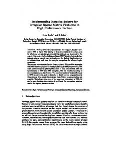
memory are connected through an element interconnect bus (EIB). The EIB consists of four buses and its total bandwidth reaches 204.8 giga bytes (GB)/sec. However, the bandwidth to the main memory is just 25.6 GB/sec. Further, that is shared by eight SPEs. Because the peak performance of an SPU on our GigaAccel 180 [9] system is 11.2 giga floatingpoint operations per second (GFLOPS), the theoretical B/F rate of the PowerXCell 8i is 0.29. The B/F rate of PowerXCell 8i is considerably smaller when I see that the B/F rate of BlueGene/L is 1.0. On the other hand, the memory bandwidth between SPU and LS is sufficiently wide. It reaches 44.8GB/sec. Although the capacity of the LS is just 256 kiro byte (KB), I must utilize this fast memory. I show the effective bandwidth between SPU and the main memory in Fig. 2. The effective transfer rate increases when the data transfer amount increases. The widest bandwidth is observed when 16KB data, the maximum size for one data transfer function call, are sent. Data transfer rate (GByte per sec.)

10

1

interest in it can be limited when I try to reduce the memory access time. Because the matrix is only needed by the matrix-vector multiplication form in CG, I do not need the matrix explicitly, although the result (e.g., q on line 11) is needed. Now, I discuss the matrix generation process of FEM. Coefficient matrices are generated by repeating the following two processes: • Generate the element-wise coefficient matrices ei, where i is the element number. • Superimpose ei on the global coefficient matrices. Therefore, if I decide to operate line 11 of the CG algorithm, I can apply the following transformation. ne  ne  q = Ap =  U e i p = U (e i p i ) . i =1  i =1 

(1)

Here, U denotes the superimposition of element wise matrices and vectors on global matrices and vectors, pi is the element wise vector of p whose components correspond to element wise matrices ei, and ne is the number of elements in a problem. When I use Equation (1), I see that the global coefficient matrix A is not explicitly needed. Moreover, I need not store ei, if I calculate them when I need them.

0.1

0.01 1 1x10

2

1x10

3

1x10

4

1x10

Data transfer amount (byte) Figure 2. The data transfer rate between the SPE and the main memory

III.

MEMORY ACCESS REDUCTION METHOD

In order for the PowerXCell 8i to achieve high performance, I must reduce the access time to the main memory. In this study, I use temporal data once and then discard them, if the same data are required repeatedly. The traditional algorithm of FEM and the access time reduction method are introduced in the following sections. A. Linear Equation Solver in FEM The FEM consists generally of two parts. One is the matrix generation part and the other is the linear equation solver. The recent development of HPC machines enables us to solve large problems. In the case of large problems of FEM, matrices have a sparse structure[7] and, therefore, iterative linear equation solvers are normally used these days [8]. The algorithm of conjugate gradient method (CG) is shown in Fig. 3. CG is one of the most well known iterative solvers and is used for various FEM implementations. In the CG algorithm, the coefficient matrix is used on line 2 and 11 as a matrix-vector multiplication form. The coefficient matrices use most of the memory space in the FEM and, therefore, most of the memory access appears in it. Then my

Figure 3. Algorithm of CG

B. Memory Access Reduction on the Cell SPUs bear a large portion of the Cell’s computational power. Therefore, I must utilize them, if I need to achieve high performance. When I use them, I must know that there are a few limitations to memory access. One is that they can only access the memory space that starts from specific addresses. The other is that their bandwidth becomes wider when the data transfer amount at one instruction becomes larger (as shown in Fig. 2). Therefore, I must rearrange the data by using the PPU, in order to transfer the data efficiently. This additional data transfer is critical for the entire performance, because the Cell does not have a good B/F rate and traditional FEM implementations require frequent memory access. Most memory access appears when

superimposing element-wise matrices and operating matrixvector multiplications. Thus, I avoid these processes by using Equation (1). C. Double Buffering Double buffering is one of the key techniques that reduce the total calculating time. SPUs can only calculate values on the LS. If they need to process data in the main memory, they must order MFCs to transfer data. Data transfer by MFCs and calculation by SPUs are completely independent. Thus, the data transfer time can be concealed behind the calculation time, especially if the calculation time is sufficiently long and the data transfer time is sufficiently short. IV.

IMPLEMENTATION

In order to evaluate our new method, I implemented the following four approaches. Traditional FEM run only on a PPU Traditional FEM using SPUs Memory access reduced FEM run only on a PPU Memory access reduced FEM using SPUs Traditional FEM holds coefficient matrices explicitly and I implemented it on the basis of GeoFEM [12], which performs well on PC clusters. GeoFEM stores coefficient matrices by using compressed row storage (CRS) format. How to use SPUs is explained in the following subsections.

SPU

SPU

LS

LS

PPU PPU

PPU PPU

Step1

Step2

SPU LS

LS

PPU PPU

PPU PPU

Step3

Step4

E-matrix2

Full matrix

Calculation with coordinate1

Coordinate2

E-matrix1

Coordinate1

Main memory

E-matrix2

Coordinate2

E-matrix1

Coordinate1

Main memory

Full matrix

SPU

Calculation with coordinate2

E-matrix2

Full matrix

Calculation with coordinate1

Coordinate2

E-matrix1

Coordinate1

Main memory

E-matrix2

Full matrix

Coordinate2

E-matrix1

Coordinate1

Main memory

A. Traditional FEM In this study, I use SPUs for matrix-vector multiplication and matrix generation, because they require the most computational effort in traditional FEMs. The brief summery of these two operations are that distribute data to SPUs by PPU, compute them in parallel on SPUs, and gather results to PPU. Concretely speaking, in matrix generation, PPU distributes coordinates of element, compute the element matrices, and superimpose them on the global matrix. In the matrix-vector multiplication, distribute row components of the global matrix and corresponding vector components, compute the product of them, and store the results to the global vector. See the details in the following sections. 1) Matrix Generation SPUs are not good at indirectly accessing the main memory. Therefore, I must prepare data on an element basis by gathering and rearranging them, before a SPU uses them. The specific contents of the prepared data are nodal coordination of an element and the components of coefficient matrices. I allocated two temporal spaces for preparation in order to perform double buffering. I illustrate the procedure of our implementation in Fig. 4. The term Coordinate and E-matrix are a nodal coordinate set of an element and element-wise coefficient matrix respectively. Arabic figures are used to identify temporal storage areas. In addition, a Full Matrix denotes the storage area for the global coefficient matrix. I explain Step 1 to Step 4 in the figure. Step1 This is the starting point of the entire calculation. The PPU stores the coordinate set of the first

elements in the temporal storage Coordinate 1. SPU obtains it immediately, and begins the calculation of the element wise matrix of the first element. Step2 PPU stores the coordinate set of the second element at Coordinate 2 during the SPU’s calculation. These operations can be done independently. Step3 PPU stores the coordinate set of the third element at Coordinate 1. The SPU stores the element-wise matrices of the first element at E-matrix1. The PPU superimposes the element wise matrix onto the global matrix. These data transfers and superimpositions are done behind the calculation of the element wise matrix of the second element. Step4 Do the same with Step 3, but use different temporal storage areas. Step3 and Step4 will be repeated until all of the elements are calculated. These procedures are carried out in parallel by using all SPUs and corresponding temporal spaces in this study. Superimposition of element-wise matrices to a global matrix can causes confliction, if I use two or more SPUs at the same time. In other words, there are dependencies in superposition in parallel computing. The confliction appears when two or more elements share a same finite element (FE) node. In order to get rid of the confliction, I employ multicoloring technique. That is to say, I divide elements into several groups whose members have no confliction with each other in a group.

Figure 4. Illustration of the matrix generation procedure using

SPU

2) Matrix-Vector Multiplication Since SPUs have limitations in memory access, I must rearrange the data when I perform the matrix-vector multiplication. In Fig. 5 at the right, I show the configuration of the temporal storage for the matrix-vector multiplication Ax=b. In the figure, Matrix, Vector, and Result with Arabic figures are temporal storage of matrix components, corresponding vector, and result of operation by SPU respectively, and Arabic figures denotes which SPU uses temporal storage. Moreover, the nonzero components of the

SPU

SPU

LS

LS

E-Vec-P2

SPU

Multiply E-mat 1 and E-Vec-P1

E-Vec-Q2

Vector-Q

Coordinate2

E-Vec-Q1

E-Vec-P1

Coordinate1

Main memory

E-Vec-P2

PPU PPU

Step2 E-mat2 construction

LS

PPU PPU

Step4

E-Vec-P2

PPU PPU

Step3

E-Vec-Q2

Vector-Q

Coordinate2

E-Vec-P1

E-Vec-Q1

Coordinate1

Main memory

E-Vec-P2

E-Vec-Q2

Vector-Q

Coordinate2

E-Vec-P1

E-Vec-Q1

B. Memory Access Reduced FEM In order to reduce the memory access time, I introduced a memory access reduced matrix-vector multiplication and double buffering in FEM. The overview of the process of multiplication is that PPU distributes coordinate information of elements, and corresponding components of vectors. SPUs compute element wise matrix-vector multiplications in parallel. Finally, PPU assembles results to the global result vector. The details of my implementation are written in the rest of this section. The developed algorithm is illustrated in Fig. 6. The figure shows a part of the matrix-vector multiplication q:=Ap, which appears in line 11 of Fig. 3. In the figure, Coordinate, E-VecP, and E-VecQ are temporal storage areas of the coordinate set of an element, element wise vector of P, and Q, respectively. In addition, Vector Q denotes the storage area for the entire q. I explain the steps in the figure. Step1 Store the coordinate set and element wise p in the temporal area Coordinate1 and E-VecP1 respectively by using PPU. SPU acquires the coordinate set as soon as possible and begins the calculation of the element wise coefficient matrix. Step2 SPU acquires the E-VecP1 during calculation of the element wise coefficient matrix. Step3 PPU stores the coordinate set and element wise p of the next element to the E-Coordinate2 and VecP2 respectively. SPU stores the result vector to EVecQ1 after the completion of the element wise matrix – vector multiplication. Step4 PPU expands E-VecQ1 to VectorQ, while SPU acquires Coordinate 2 and begins the calculation. Step2 to Step4 repeats, using temporal areas 1 and 2 in alternation, until all of the elements have been calculated. The outlook of this procedure is somewhat similar to the procedure of global coefficient matrix generation (Section 4-

PPU PPU

LS

Coordinate1

Figure 5. Illustration of the matrix-vector multiplication

E-mat1 construction

Step1 SPU

Main memory

Main memory

E-Vec-Q2

Vector-Q

SPU4 LS

Coordinate2

E-Vec-Q1

E-Vec-P1

…

…

PPU PPU

A ・ x= b

Matrix4 Vector4 Result4

SPU1 LS

Coordinate1

Matrix1 Vector1 Result1

A-1). However, the memory access amount of this procedure is significantly less than that of the global coefficient matrix generation. In fact, the memory access amount of this procedure is proportional to nm, while that of the global matrix generation is proportional to n2m, where n is the dimension of the element wise matrix and m is the number of elements.

Main memory

global matrix and vector are shown as hatched squares. In this study, I employ the CRS storage format to store the global matrix. Therefore, the Matrix storage areas store the single rows and Vector storage areas store the corresponding vector components. Since the operations of a row and other rows are independent, I can apply parallel computation without difficulty. In the figure, SPU1 and SPU4 compute at the same time and other SPEs can do the same. In order to obtain high performance, double buffering technique is employed.

Figure 6. Illustration of memory access time reduction FEM

V.

PERFORMANCE EVALUATION

In order to evaluate the performance of my new implementation, the calculation times for each implementation were measured. Conditions are described in the following section, and calculation times are tabulated in the section after the next session. A. Measurement Conditions In this study, I solved Poisson equation on a three dimensional cubic domain. The analysis domain is discretized using first-order 8-noded elements. The shape of elements is uniform. However, I do not apply any specialization. Therefore, I can discuss following result without loss of generality. I prepare four cases by changing the number of total elements (83, 163, 323, and 643). I set value 0 on a face of cube and value 100 on the opposite face as Dirichlet boundary condition. B. Calculation time Calculation times of each implementation are tabulated in Table 1. Calculation times for matrix generation (Mat. Gen.) and CG are also tabulated for traditional FEM. Because memory access reduced FEM includes matrix generation in CG iteration, calculation time of memory access reduced FEM should be compared with the total calculation time of traditional FEM. In this section, I used eight SPUs. The memory access reduced FEM on SPU is the fastest in all cases (6.60x10-3, 9.17x10-2, 1.97, and 2.9x101 sec.). The second fastest is the traditional FEM on PPU (1.78x10-2, 3.85x10-1, 9.30x100, and 2.62x102 sec.). The third is the traditiona FEM on SPU (2.06x10-2, 2.79x10-1, 3.44x101, and 4.25x102 sec.). The last is the memory access reduced FEM

TABLE I.

CALCULATION TIMES FOR EACH IMPLEMENTATION.

Implementation Traditional FEM on PPU Traditional FEM on SPU

Mat. Gen.

83

163

323

643

1.48E-2

3.10E-1

8.04E+0

2.43E+2

CG

3.01E-3

7.52E-2

1.26E+0

1.89E+1

Total

1.78E-2

3.85E–1

9.30E+0

2.62E+2

Mat. Gen.

1.04E-2

1.15E-1

1.04E+0

8.80E+0

CG

1.02E-2

1.64E-1

2.40E+0

3.47E+1

Total

2.06E-2

2.79E-1

3.44E+0

4.25E+1

8.09E–2

1.28E+0

2.06E+0

3.01E+2

6.60E–3

9.17E–2

1.97E+0

2.90E+1

15

26

48

86

2.00E-4

2.89E-3

2.62E-2

2.20E-1

3.53E-3

4.11E-2

3.38E-1

Memory Access Reduced FEM on PPU Memory Access Reduced FEM on SPU Number of Iterations CG/iter. of Traditional FEM on PPU CG/iter. of Memory Access Reduced FEM on SPU

4.40E-4

Moreover, matrix generation of traditional FEM on SPU is faster than that on PPU. Therefore, it can be said that the matrix generation is suitable for the Cell processor. On the other hand, CG on SPU is slower than that on PPU. It caused by the extra data copy for data transfer to SPUs. Now, I introduce the parallel performance of SPU implementations. Calculation times of each problem size by changing the number of SPUs are shown in from Fig.7 to Fig. 10. Figure 7 to 10 are the plots of the calculation time in the case of the total number of elements are 83, 163, 323, and 643, respectively. Except the case of 83, Traditional FEM is faster than Memory Access Reduced FEM when I use only one SPU. It implies that if the wider memory bandwidth I can obtain, traditional FEM works better. However, when the number of SPUs increases memory access reduced FEM shows better performance. Eventually, when I use at lease four SPUs, memory access reduced FEM shows better performance than traditional FEM. VI.

Unit: seconds, except number of iterations

on PPU (8.09x10-2, 1.28x10-1, 2.06x101, and 3.01x102 sec.). The times in parentheses are calculation time for each problem size, respectively. The memory access reduced FEM on SPU is the fastest while it on PPU is the slowest. This fact shows that the memory access reduced FEM does not reduce computational efforts but it achieves good performance on SPU.

A. Comparison of Computational Efforts In this section, I theoretically compare the amount of computations and data transfer between traditional FEM and memory access reduced FEM. In this section, I consider the same analysis domain and meshes with that are used in section V. Moreover, I only consider the matrix-vector multiplication y:=Ax, because it requires the largest 0

-2

7.0x10

3.0x10

Traditional FEM Memory Access Reduced

-2

-2

2.0x10

-2

1.5x10

-2

0

4.0x10

0

3.0x10 2.0x10

0

1.0x10

-3

1

2

3

4 5 6 Number of SPUs

7

8

1

2

3

4 5 6 Number of SPUs

7

8

Figure 9. Calculation time for 323 elements.

Figure 7. Calculation time for 83 elements.

2

1.0x10

-1

4.5x10

Traditiona FEM Memory Access Reduced

1

Traditional FEM Memory Access Reduced

-1

4.0x10

9.0x10

3.5x10-1

Time for calculation

Time for calculation

0

5.0x10

0

1.0x10

-1

3.0x10

-1

2.5x10

-1

2.0x10

-1

1.5x10

1

8.0x10

1

7.0x10

1

6.0x10

1

5.0x10

1

4.0x10

1

-1

3.0x10

1.0x10

1

-2

5.0x10

Traditional FEM Memory Access Reduced

0

6.0x10

Time for calculation

Time for calculation

2.5x10

5.0x10

DISCUSSIONS

1

2

3

4 5 6 Number of SPUs

7

Figure 8. Calculation time for 163 elements.

8

2.0x10

1

2

3

4 5 6 Number of SPUs

7

Figure 10. Calculation time for 643 elements.

8

computational efforts in most iterative solvers. Firstly, I consider the traditional FEM. Because I use the same meshes that are used in section V, I can estimate that the number of non-zero element of a row of coefficient matrices is 27, when the total number of element ne is sufficiently large. Therefore, the number of floating point number operations(FLOP) NTradFLOP is written as, Trad (2) N FLOP = (27(mul.) × 26(add )) × n , where n is the total number of FE nodes. In addition, the amount of data transfer NTradmemory is written as, Trad N FLOP = 27 × {8bytes(non - zero elements of matrix )

+ 4bytes(CRS index )

.(3)

+ 8bytes(vector x )}× n However, I do not take it into consideration that the data copy which is required to the use of SPUs. When I substitute n=83 to Equation (2) and (3), I obtain NTradFLOP=27,136, NTradmemory=276,480byte. On the other hand, if I consider the number of FLOP NMemReduceFLOP, and the amount of data transfer NMemReducememory of memory access reduced FEM, they are written as follows: Mem Re duce (4) N FLOP = 2810(FLOP per element ) × ne , and Mem Re duce N memory = {[4bytes(node index )

+ 3 × 8bytes(coordinate of a node)

+ 16bytes(vector x, and vector y )] × 8(number of nodes in a element )}× ne

.

(5)

When n is 83, ne becomes 343. I substitute ne=343 to Equation (4) and (5), and I obtain NMemReduceFLOP=895,230, and NMemReducememory=120,736byte. By comparing obtained results, memory access reduced FEM requires around 30 times more calculations than traditional FEM. On the other hand, memory access reduced FEM only requires lesser than the half of the data transfer amount of traditional FEM. B. Calculation Performance The computational cost of CG of traditional FEM and memory access reduced FEM are not same with each other. In this section, I evaluate the computational cost per CG iteration of both implementations and discuss the effective range of memory access reduced FEM. Therefore, in the remaining of this section, I focus on the comparison of traditional FEM on PPU and memory access reduced FEM on SPU. In Table I, I tabulate the number of iterations to the CG convergence and computational time of each implementation and problem size. In the case of traditional FEM, calculation times for matrix generation are also shown. Calculation times for matrix generation of traditional FEM on PPU with each problem are 1.48x10-2 sec., 3.10x10-1 sec., 8.04x100 sec., and 2.43x102 sec. Calculation times for CG are 3.01x10-3 sec., 7.52x10-2 sec., 1.26x100 sec., and 1.89x101 sec. Numbers of iterations to the CG convergence are 15, 26, 48, and 86. Therefore, computational times per CG iteration are 2.00x10-4 sec., 2.89x10-3 sec., 2.62x10-2 sec., and 2.20x10-1 sec. On the other hand, calculation times for CG of memory access reduced FEM are 4.40x10-4 sec.,

3.53x10-3 sec., 4.11x10-2 sec., and 3.38x10-1 sec. The computation cost of one CG iteration of memory access reduced FEM on SPU is higher than that of traditional FEM on PPU. However, memory access reduced FEM shows better performance than traditional FEM in this study. This is because the memory access reduced FEM does not require explicit matrix generation process. By considering above results, memory access reduced FEM shows better performance, if the numbers of iterations to the CG convergence are smaller than 62, 490, 539, or 2064, respectively. It can be said that the bigger problem size becomes, the wider effective range of memory access reduced FEM becomes. In Table II, I tabulate the calculation times, the effective FLOPS, and the effective to peak performance ratio (percentage) of matrix-vector multiplication for each implementation and problem size. The peak performance of 1SPU is 11.2 GLOPS and 8SPU reaches 90 GFLOPS. The peak performance of PPU is 5.6GFLOPS. The FLOPS values in the table are calculated using the result of section VI-A. Traditional FEM on SPU shows around 30MFLOPS on one SPU (0.3% of the peak), and 40FLOPS on eight SPUs (0.06% of the peak). Not only are the effective to the peak performance ratio, but also the FLOPS of SPU implementations lower than that of PPU implementation (around 70MFLOPS, 1.3% of the peak). It implies that the data transfer in SPU implementations consumes the most of calculation time. On the other hand, memory access reduced FEM shows around 0.7GFLOPS (6% of the peak) on one SPU, and around 2GFLOPS (2.4% of the peak) on eight SPUs. Therefore, the utilization efficiency of SPUs of memory access reduced FEM is better than that of traditional FEM. Moreover, the FLOPS value on SPU becomes better than that on PPU (around x3.5 on one SPU, x10 on eight SPUs). Therefore, memory access reduced FEM is suitable implementation for the Cell processor. In order to confirm that the memory access reduced FEM reduces or conceal the memory access time than traditional FEM, I measure the actual data transfer time and calculation time, and compared them with the entire matrix-vector multiplication. These measurements are carried out by using SPU implementation only and one SPU is used, because I can measure pure data transfer time and calculation time. Moreover, the smallest problem size (the total number of nodes is 83) is used in this discussion. Firstly, I consider the memory access reduced FEM. In the memory access reduced FEM, the data transfer time per element on a SPU is 0.98x10-6 sec. Pure calculation time on a SPU is 2.10x10-6 sec. By multiplying the total number of elements (343 when the total number of nodes is 83) to the sum of those, I obtain 1.06x10-3sec. The entire of matrix-vector multiplication by one SPU is 1.47x10-3 sec. The rest (0.31x10-3 sec.) is used by PPU for the preparation to the data transfer to a SPU. On the other hand, in the traditional FEM, the data transfer time per node is 0.35x10-6, and calculation time is 0.07x10-6. By multiplying the number of nodes to the sum of those, I obtain 0.25x10-3 sec. The entire calculation time of matrix-vector multiplication is 0.89x10-3 sec, thus, PPU uses 0.64x10-3 sec. In the Cell processor, PPU and SPUs are completely

independent with each other. Therefore, if the time for PPU operation is shorter than that for SPU operation, I can conceal the entire of the preparation time by PPU. On this point, the preparation time of memory access reduced FEM is just 20% of the entire, but for the traditional FEM, it reaches 70%. Since the preparation time by PPU corresponds to sequential part in the Amdahl’s low, the effect of parallel computation of SPUs becomes better when the preparation time is shorter. Consequently, memory access reduced FEM is more suitable for the Cell processor than the traditional FEM. TABLE II.

EFFECTIVE FLOPS OF MATRIX-VECTOR MULTIPLICATION OF EACH IMPLEMANTATION.

Implementation Traditional FEM on SPU (1SPU) Memory Access Reduced FEM on SPU (1SPU) Traditional FEM on SPU (8SPU) Memory Access Reduced on SPU (8SPU) Traditional FEM on PPU Memory Access Reduced FEM on PPU

83 8.90E-4 3.13E+7 0.28 1.47E-3 6.79E+8 6.06 5.24E-4 5.18E+7 0.06 4.54E-4 2.12E+9 2.36 1.85E-4 1.47E+8 2.62 5.23E-3 1.84E+8 3.29

163 7.07E-3 3.07E+7 0.27 1.37E-2 6.90E+8 6.16 5.45E-3 3.98E+7 0.04 3.87E-3 2.60E+9 2.89 2.81E-3 7.73E+7 1.38 4.87E-2 1.95E+8 3.48

323 5.60E-2 3.10E+7 0.28 1.20E-1 6.96E+8 6.22 4.46E-2 3.89E+7 0.04 3.93E-2 2.13E+9 2.37 2.48E-2 7.01E+7 1.25 4.33E-1 1.94E+8 3.46

643 4.50E-1 3.09E+7 0.28 1.00E+0 6.99E+8 6.24 3.66E-1 3.79E+7 0.04 3.26E-1 2.16E+9 2.40 2.09E-1 6.66E+7 1.19 3.63E+0 1.93E+8 3.45

Units of each cell, Top: calculation time, Middle: FLOPS, Bottom: effective to peak performance ratio (%)

C. Memory Usage Estimation Because the memory access reduced FEM does not require global coefficient matrix, it uses lesser memory than the traditional FEM. In this section, I estimate the amount of memory usage for both implementations. I consider the same conditions with section V (8-noded first order element and cubic analysis domain). Almost of memory space are used by the following data: 1. Coordinates of FE nodes (3 x n x 8bytes). 2. Element connectivity (8 x n x 4bytes). 3. Temporal vectors for CG (5 x n x 8bytes). 4. *Non-zero element of a matrix (27 x n x 8bytes). 5. *CRS index of a matrix (27 x n x 4bytes). Where, n is the number of FE nodes in an analysis system, and values in parentheses are the amount of data. I suppose that the number of element is equivalent to the number of nodes. The symbol “*” indicates that items required only for the traditional FEM. After a simplification, traditional FEM requires around 460 x n bytes and memory access reduced FEM requires 100 x n bytes. Simply, I can analyze 4.5 time bigger problems than traditional FEM for Poisson like equations. Additionally, if the degree of freedom per node increases, the difference of memory usage between memory access reduced FEM and traditional FEM increase.

VII. RELATED WORKS In the references[9][10], sparse matrix-vector multiplication programs were implemented on the Cell processor, AMD Opteron, Intel Itanium, and Cray X1E. Sparse matrices were stored by using CRS format. The Cell processor used in the literatures did not have enhanced double precision units. In other words, its peak performance was 204.8 GFLOPS for single precision operation, and 14.63 GFLOPS for double precision operation. In the literature, Williams et al. obtained 3.59GFLOPS (1.75% of the peak) for single precision and 2.5GFLOPS (17.1% of the peak) for double precision. In addition, they obtained 6.02% of the peak for single precision and 8.18% of the peak for double precision on AMD Opteron that is one of typical scalar processor. By comparing these results, calculation efficiency for double precision on the Cell looks excellent. However, FLOPS for single precision was just the double of FLOPS for double precision. That can be explained by using the difference of the amount of data. Briefly speaking, the amount of data for double precision case is double of single precision case and the effect of memory bandwidth is dominant factor in the performance of sparse matrix-vector multiplication. The relative performance of the Cell was worse than that of Opteron, while peak performance of the Cell is quite better. The gap between calculation performance and memory bandwidth will increase. Therefore, I must develop new framework for the future processors. In addition, cache blocking technique that increases the effect of LS and cache memory in the literature, in order to obtain better performance. The effect of cache blocking is significant, when my traditional FEM implementation on PPU shows just 2% of the peak, while they achieve 8% of the peak. However, the effect of cache blocking can be smaller when the problem size becomes bigger. Their biggest problem was 75,000 degree of freedom, while my biggest problem was 260,000. They estimated that the upper limit of the performance without cache blocking was 0.35GFLOPS for single precision. Therefore, it should be 0.18 GFLOPS for double precision. The effective performance of their implementation will approach to that limit when the problem size increases. Coefficient matrix reduced approaches have been developed in order to reduce the memory usage [11][14]. However, in the reference [11], Okuda reduced computational efforts on the sacrifice of calculation accuracy. Additionally, in reference [14], Arbenz et al. assumed that all elements were uniform and they need not re-compute element coefficient matrix. VIII. CONCLUSIONS In this study, I implemented memory access reduced FEM solver in order to increase the execution efficiency on low B/F rate processor. The performance of memory access reduced FEM was compared with the traditional FEM that stored coefficient matrix by using CRS format. Additionally, both implementations were evaluated on PPU that is equivalent to PowerPC scalar processor and SPUs that is a kind of chip multi processor. As a result, memory access

reduced FEM on SPU (calculated within 2.90 x 101 sec.) showed ten times better performance than the traditional FEM on PPU (2.64 x 102 sec.). Memory access reduced FEM reduces memory access times by accepting additional floating-point operations by not storing data if it is required repeatedly. Therefore, memory access reduced FEM is suitable for future processors, because they will have a bigger gap between computational performance and memory bandwidth than current processors. In addition, memory access reduced FEM enables us to solve bigger problems. By my estimation, I can solve five times larger problem if I solve Poisson equation. I only solved Poisson equation and only used CG in this study. However, the discussion can be extended for other problems without difficulty. For example, I observed that the parallel performance saturated when the number of SPUs was four. Therefore, if I use elements that require more computations per element, parallel performance will become better. Second order 20-noded element requires 20 times more calculations than first order 8-noded element, while it requires only 3 times more data transfer. Moreover, memory access reduced FEM is more suitable for the problems that use coefficient matrix only one time than traditional FEM (In the reference [13], coefficient matrices are non-linear and they change their contents in each CG iteration). For the future works, I must develop efficient preconditioning technique, because memory reduced access FEM will be slower than traditional FEM, when the number of iterations to the CG convergence increases. ACKNOWLEDGMENT I am grateful to JSPS for the Grant-in-Aid for Young Scientists (B), No. 21760701. I also thank A. Tomita and K. Fujibayashi @FIXSTARS Co. for their extensive knowledge of the CELL. REFERENCES [1]

[2]

[3] [4] [5]

[6]

[7] [8]

International Business Machines Corporation, Sony Computer Entertainment Incorporated, and Toshiba Corporation Cell Broadband Engine Architecture, Version 1.01, 2006. J. Gebis, L. Oliker, J. Shalf, S. Williams, K. Yelick, “Improving Memory Subsystem Performance using ViVA: Virtual Vector Architecture”, ARCS: International Conference on Architecture of Computing Systems, Delft, Netherlands, March 2009. Top500 supercomputer sites, http://www.top500.org, 2010. Roadrunner web site, http://www.lanl.gov/roadrunner/, 2008. N. Kushida, and H. Okuda, “Optimization of the Parallel Finite Element Method for the Earth Simulator”, Journal of Computational Science and Technology, vol.2, No. 1, 2008, pp 81-90. M. Satoh, T. Matsuno, H. Tomita, H. Miura, T. Nasuno, and S. Iga, Nonhydrostatic Icosahedral Atmospheric Model (NICAM) for global cloud resolving simulations, Journal of Computational Physics Vol.227, 2008, pp. 3486-3514. O. C. Zienkiewicz, and K. Morgan, “Finite Elements and Approximation”, A Wiley-interscience Publication, 1983. Y. Saad, “Iterative Methods for Sparse Linear Systems second edition”, SIAM, 2003.

[9]

[10]

[11]

[12]

[13]

[14]

S. Williams, J. Shalf, L. Oliker, S. Kamil, P. Husbands, and K. Yelick, “Scientific Computing Kernels on the Cell Processor”, International Journal of Parallel Programming, vol. 35, 2007, pp. 263-298. S. Williams, J. Shalf, L. Oliker, S. Kamil, P. Husbands, and K. Yelick, “The potential of the cell processor for scientific computing”, Proceedings of the 3rd conference on Computing frontiers, ACM Press, 2006, pp. 9-20. Y. Nakabayashi, G. Yagawa, and H. Okuda, “Parallel finite element fluid analysis on an element-by-element basis”, Computational Mechanics, Vol. 18, No. 5, 1996, pp. 377-382. H. Okuda, and G. Yagawa, “Large-Scale Parallel Finite Element Analysis for Solid Earth Problems by GeoFEM”, Surveys on Mathematics for Industry, Vol.11, No.1-4, 2005, pp. 159-196. N. Kushida, and H. Okuda, “Finite Differential Approximated Hessian Preconditioner for non-linear conjugate gradient methods: For Ab-inition Calculations”, Transacsions of The Japanese Society for Computational Engineering and Science, 2004, No.20040023. (In Japanese) P. Arbenz, G. H. Van Lenthe, U. Mennel, R. Müller, and M. Sala, “Multi-level µ-finite element analysis for human bone structures”, Proceedings of the 8th international conference on Applied parallel computing: state of the art in scientific computing, 2006, pp. 240-250.