Em*: a Software Environment for Developing and ... - CiteSeerX

Em*: a Software Environment for Developing and Deploying Wireless Sensor Networks Lewis Girod Jeremy Elson Alberto Cerpa Thanos Stathopoulos Nithya Ramanathan Deborah Estrin Center for Embedded Networked Sensing University of California, Los Angeles Los Angeles, CA 90095 USA {girod,jelson,cerpa,thanos,nithya,destrin}@cs.ucla.edu

Abstract Em* is a software environment for developing and deploying Wireless Sensor Network (WSN) applications on Linux-class hardware platforms (called “Microservers”). Em* consists of libraries that implement message-passing IPC primitives, tools that support simulation, emulation, and visualization of live systems, both real and simulated, and services that support for networking, sensing, and time synchronization. While Em*’s design has favored ease of use and modularity over efficiency, the resulting increase in overhead has not been an impediment to any of our current projects.

1

Introduction

The field of wireless sensor networks (WSNs) is growing in importance,[1] with new applications appearing in the commercial, scientific, and military spheres, and an evolving family of platforms and hardware. One of the most promising signs in the field is a growing involvement by researchers outside the networking systems field who are bringing new application needs to the table. A recent NSF Workshop report[8] details a number of these needs, building on early experience with deployments (e.g. GDI[15], CENS[20], James Reserve[23]). Many of these applications lead to “tiered architecture” designs, in which the system is composed of a mixture of platforms with different costs, capabilities and energy budgets.[3][18] Low capability nodes, often Crossbow Mica[21] Motes running TinyOS[12] can perform simple tasks and provide long life at low cost. The high capability nodes, or microservers, generally consume more energy, but in turn can run more complex software and support more sophisticated sensors. Em*1 is a software environment targeted at microserver platforms. Microservers, typically iPAQ or Crossbow Stargate platforms, are central to several new applications at CENS. The Extensible Sensing System (ESS) employs microservers as data sinks to collect and report microclimate data at the 1 The Em* name derives from a number of its tools and services whose names begin with “Em” for “embedded”.

James Reserve. A proposed 50-node seismic network will use Stargates to measure and report seismic activity using a high-precision multichannel ADC. Ongoing research in acoustic sensing uses iPAQ hardware to do beamforming and animal call detection. WSNs have several properties that distinguish them from other types of distributed systems. First, the system as a whole must often be energy-aware. Two important factors in energy consumption are communication, because physics dictates strict lower bounds on the energy required, and RAM, because existing technology requires energy to refresh it. Duty cycling is an important technique to reduce energy requirements. Second, WSNs are often forced, for reasons of cost and energy, to use low capability communications, which tend to have reduced range, bandwidth and reliability, and higher latency. Third, because of the poor comms and the need to save energy, systems often must implement distributed algorithms through multihop in-network processing. In addition, in-network collaboration and triggering can yeild results that would be impossible with a centralized system. Fourth, WSN applications often encounter a high degree of environmental dynamics, requiring a reactive system design. In this paper, we will show how Em* addresses many of these needs in support of WSN application development. 2

2

Tools and Services

Em* incorporates a number of tools and services germane to the creation of wireless sensor network applications. In this section, we will briefly describe these, without going into detail about their implementation. In Section 3, we will detail some of the key building blocks used to construct them. Then, in Section 4 we return to our tools and services and show how their implementation made use of these building blocks. 2 This work was made possible with support from the NSF Cooperative Agreement CCR-0120778, and the UC MICRO program (grant 01-031) with matching funds from Intel Corp. Additional support was provided by the DARPA NEST program (the “GALORE” project, grant F3361501-C-1906).

imizing parallelism. EmRun also maintains a control channel to each child process that enables it to monitor process health (repawn dead or stuck processes), initiate graceful shutdown, and receive notification when starting up that initialization is complete. Log messages emitted by Em* services are processed centrally by EmRun and exposed to interactive clients as in-memory logrings with runtimeconfigurable loglevels. Figure 1:

2.1

2.2 (a) EmView and (b) the Ceiling Array

Em* Tools

Em* tools include support for deployment, simulation, emulation, and visualization of live systems, both real and simulated. EmSim/EmCee The ability to transparently simulate at varying levels of accuracy is critically useful for building and deploying large systems.[6] Together, EmSim and EmCee comprise several accuracy regimes. EmSim is a pure simulation environment, in which many virtual nodes are run in parallel, interacting with a simulated environment and radio channel. EmCee runs the EmSim core, but provides an interface to real low-power radios instead of a simulated channel. These simulation regimes speed development and debugging; pure simulation helps to get the code logically correct, while emulation in the field helps to better understand environmental dynamics before a real deployment. While simulation and emulation don’t obviate the need for debugging a deployed system, they will tend to reduce the number of problems that arise in it. In all of these regimes, the running Em* binaries are identical, making it painless to transition among them during development and debugging, and eliminating the accidental code differences that can arise when running in simulation requires modifications. EmSim is similar to other “real-code” simulation environments, such as TOSSim[14]. EmView/EmProxy EmView is a graphical visualizer for Em* systems. It is designed to be easily extended to support new visualization needs as they arise. EmView can request and capture status updates from a collection of nodes, or from a simulator. Because it uses UDP, the requests can be broadcast to a group of nodes, and the responses arrive with low latency, enabling EmView to capture realtime system dynamics. EmProxy is a server that runs on a node or as part of a simulation, and handles requests from EmView. Based on the request, EmProxy will monitor specific status interfaces and immediately report any changes on those interfaces back via UDP. EmRun EmRun is a service responsible for starting, stopping, and managing an Em* system. It processes a config file that specifies how the Em* services are “wired” together, and starts the system up in dependency order, max-

Em* Services

Em* services include support for networking, sensing, and time synchronization. Link and Neighborhood Esimation The LinkStats and Neighbors services monitor a radio link to estimate connectivity to other nodes on the same channel, and expose this information to their clients. When significant changes occur, the clients are notified so that they can take necessary action. This information is useful for two reasons. First, many systems need to know their directly connected neighbors because they need to interact or collaborate with them. Neighbors provides them a list of neighbors and enables them to select which they want to use based on link quality or other metrics. Notification of changes enables them to quickly react to a changing environment. Second, wireless systems have a significant “gray zone” where connectivity is poor and unreliable[2]. Some algorithms choose to ignore these links, while others factor link quality into their algorithms. For example a routing algorithm might use a metric that uses link quality to weight hop counts. Time Synchronization The ability to relate the times of events on different nodes is critical to most distributed sensing applications, especially those interested in correlation of high-frequency phenomena. The TimeSync service provides a mechanism for converting among CPU clocks (i.e. gettimeofday()) on neighboring nodes. Rather than attempt to synchronize the clocks to a specific “master”, TimeSync estimates conversion parameters that enable a timestamp from one node to be interpreted on another node. Timesync can also compute relations between the local CPU clock and other clocks in the system such as sample indices from an ADC or the clocks of other processor modules. Routing Em* supports several types of routing: Flooding, Geographical, and Quad-Tree. One of the founding principles of Em* is that innovation in routing, and hybrid transport/routing protocols are key research areas in the development of wireless sensor network systems. Thus, while Em* “supports” several routing protocols, the point is that it’s easy to invent your own. For example, the authors of Directed Diffusion [11][13] are implementing their protocol for Em*.

2.3

Em* Device Support

Em* includes native support for a number of devices, including sensors, and radio hardware.

HostMote and MoteNIC Em* systems often need to gateway to a network of low-energy platforms such as Mica[21] Motes running TinyOS[12]. To enable this, the HostMote service implements a line protocol to a compatible Mote attached to an Em* node via a serial port. The HostMote service provides a configuration interface and a message interface that demultiplexes traffic to and from the Mote to multiple clients. MoteNIC is a packet relay service that connects to HostMote. MoteNIC provides a standard Em* data link interface, and translates messages to and from the Mote. Software on the Mote then relays those packets onto the air. Audio Server The Audio service provides a buffered and continuous streaming interface to audio data sampled by sound hardware. It also propagates synchronization information to the TimeSync service to enable clients to use TimeSync to relate specific sample indices to CPU times. Using the Audio service, clients can extract data from a buffer of historical data as well as receive a stream of data as it arrives. The ability to acquire historical data is crucial to implementing triggering and collaboration algorithms where there may be a significant nondeterministic delay in communication due to channel contentention, multihop communication, duty cycling, and other sources of delay. Other Sensor Hardware We have implemented a number of other services that support various sensor devices we have encountered. For the NIMS project, we have built a driver for the DGH multichannel ADC conversion module. We have also built a driver for the WMR968 weather station.

3

Building Blocks

In this section, we will describe in more detail the building blocks that enabled us to construct the Em* suite of tools and services. The basic structure of Em* encapsulates logically separable modules within individual processes, and enables communication among these modules through message passing via device files. This structure provides for fault isolation and independence of implementation among services and applications. In principle, Em* does not specify anything about the implementation of its modules, apart from the POSIX system call interface required to access device files. For example, most Em* device interfaces can be used interactively from the shell, and Em* servers could be implemented in any language that supports the system call interface. In practice, there is much to be gained from using and creating standard libraries. In the case of Em* we have implemented these libraries in C, and we have adopted the GLib event framework to manage select() and to support timers. The event framework enables us to encapsulate complex protocol mechanisms in libraries, which we can then conveniently integrate without explicit coordination. The decision to use C, GLib, and the POSIX interface was designed to minimize the effort required to integrate Em*

with arbitrary languages, implementation styles, and legacy codebases. We will now describe some key building blocks in more detail. These building blocks, the Em* IPC mechanisms and associated libraries, will be explained in terms of what they do, how they work, and how they are used.

3.1

FUSD

FUSD, the Framework for User-Space Devices, is essentially a microkernel extension to Linux. FUSD allows device-file callbacks to be proxied into user-space and implemented by user-space programs instead of kernel code. Though implemented in userspace, FUSD drivers can create device files that are semantically indistinguishable from kernel-implemented /dev files, from the point of view of the processes that use them. FUSD follows in the tradition of microkernel operating systems that implement POSIX interfaces, such as QNX [26] and GNU HURD [22]. A performance analysis of Em*’s FUSD–based interfaces appears in Section 3.3.2. As we will describe in later sections, this capability is used by Em* modules for both communication with other modules and with users. Of course, many other IPC methods exist in Linux, including sockets, message queues, and named pipes. We have found a number of compelling advantages in using using user-space device drivers for IPC among EmStar processes. For example, system call return values come from the EmStar processes themselves, not the kernel; a successful write() guarantees that the data has reached the application. Traditional IPC has much weaker semantics, where a successful write() means only that the data has been accepted into a kernel buffer, not that it has been read or acknowledged by an application. FUSD-based IPC obviates the need for explicit applicationlevel acknowledgement schemes built on top of sockets or named pipes. FUSD-driven devices are a convenient way for applications to expose state or configuration variables in a convenient, browseable, named hierarchy—just as the kernel itself uses the /proc filesystem. These devices can respond to system calls using custom semantics; for example, a read from a packet-interface device (Section 3.2.2) will always begin at a packet boundary. The customization of system call semantics is a particularly powerful feature, allowing surprisingly expressive APIs to be constructed. We will explore this feature further in Section 3.2. 3.1.1

FUSD Implementation

The proxying of kernel system calls is implemented using a combination of a kernel module and cooperating userspace library. The kernel module implements a device, /dev/fusd, which serves as a control channel between the two. When a user-space driver calls fusd register(), it uses this channel tell the FUSD kernel module the name of the device being registered. The FUSD kernel module, in turn, registers that device with the kernel proper using de-

vfs, the Linux device filesystem. Devfs and the kernel don’t know anything unusual is happening; it appears from their point of view that the registered devices are simply being implemented by the FUSD module. FUSD drivers are conceptually similar to kernel drivers: a set of callback functions called in response to system calls made on file descriptors by user programs. In addition to the device name, fusd register() accepts a structure full of pointers to callback functions, used in response to client system calls—for example, when another process tries to open, close, read from, or write to the driver’s device. The callback functions are generally written conform to the standard definitions of POSIX system call behavior. In many ways, the user-space FUSD callback functions are identical to their kernel counterparts. When a client executes a system call on a FUSDmanaged device (e.g., open() or read(), the kernel activates a callback in the FUSD kernel module. The module blocks the calling process, marshals the arguments of the system call, and sends a message to the user-space driver managing the target device. In user-space, the library half of FUSD unmarshals the message and calls the user-space callback that the FUSD driver passed to fusd register(). When that user-space callback returns a value, the process happens in reverse: the return value and its side-effects are marshaled by the library and sent to the kernel. The FUSD kernel module unmarshals the message, matches it with the corresponding outstanding request, and completes the system call. The calling process is completely unaware of this trickery; it simply enters the kernel once, blocks, unblocks, and returns from the system call—just as it would for a system call to a kernel-managed device. One of the primary design goals of FUSD is stability. A FUSD driver can not corrupt or crash any other part of the system, either due to error or malice. Of course, a buggy driver may corrupt itself (e.g., due to a buffer overrun). However, strict error checking is implemented at the user/kernel boundary which prevents drivers from corrupting the kernel or any other user-space process—including other FUSD drivers, and even the processes using the devices provided by the errant driver.

3.2

Device Patterns

Using FUSD, it is possible to implement character devices with more or less arbitrary semantics. FUSD itself does not enforce any restrictions on the semantics of system calls, other than those needed to maintain fault isolation between the client, server, and kernel. While this absence of restriction makes FUSD a very powerful tool, we have found that in practice the interface needs of most applications fall into well-defined classes. We use the term Device Pattern to refer to these interface classes. We call them “patterns” because they factor out the semantics of the device common to a class of interfaces, while leaving the rest to be customized in the implementation of the service. The Em* device patterns are implemented by libraries

that include hooks into the GLib event framework. These hooks enable them to encapsulate the detailed interface to FUSD, leaving the service to provide only configuration parameters and the minimal set of callback functions required to customize the semantics of the device to fit the application. For example, the Status Device pattern defines the behavior when the device is read, but requires that the application provide a callback to represent the application’s current “status” on demand. A key property of Em* device patterns, relative to other approaches such as log files and status files, is their active nature. For example, the Logring Device pattern appears very much like a log file, but it stores only recent log messages in memory, and reports them followed by a stream of new messages as the arrive. The Status Device pattern appears very much like a file that always contains the most recent state of the service providing it. However, most status devices also support poll()-based notification of changes to the state. The following sections will describe the Device Patterns defined within Em*. Most of these patterns were discovered during the development of services that needed them, and later factored out into libraries. In some cases, several similar instances were discovered, and the various features amalgamated into a single pattern. 3.2.1

Status Device

The Status Device pattern provides a device that always reports the current state of the service providing it. The exact semantics of “state” is determined by the service; there is no limitation on the number of separate Status Devices employed by a single service. The data reported by a Status Device is not limited in size to a single read(). The Status Device reports its data using a simple protocol in which multiple sequential reads may be completed, terminated by a zero-length read to indicate the end of the status report. Status Devices are used for a wide variety of purposes, including the output of a neighbor discovery service and the current configuration and packet transfer statistics for a radio link. Because they are so easy to integrate into an Em* service, they are also favored for output of a wide variety of debugging information. Server w rite

status_notify()

binary printable

Server

pd_unblock()

Packet Device

pd_receive() send

O F

Status Device

O

Client1

Figure 2:

filter

I F

F

I I

Client2

Client3

O

Client1

I

O

Client2

I

O

Client3

Block diagram of the (a) Status and (b) Packet Device patterns. In the Packet Device diagram, the “F” boxes are client-configurable filters, and the curved arrows from Client1 represent ioctl() based configuration of queue lengths and message filtering.

While it is often convenient to use cat to interactively view the state of a service from the shell, an important feature of the Status Device is its support for “binary mode”. A client can put the device into binary mode using a special ioctl() call. After this call is performed, the device will produce output formatted in service-specific structs rather than human-readable ASCII. For programmatic use, binary mode is preferable for reasons of both convenience and compactness. In addition to polling the state by reading the device, Status Device supports change notification through poll(). When the service’s state changes, the service can choose to notify its clients, causing their devices to become readable. Upon notification, each client can read it again to receive the updated state information. This process highlights another key property of the status device: while every read is guaranteed to compute and report the current state, the client is not guaranteed to see every intermediate state transition. The corollary to this is that if no clients care about the state, no work is done to compute it. Applications that desire queue semantics should use the Packet Device pattern (described in Section 3.2.2). Another feature of Status Device is support for multiple concurrent clients. Although intended to support one-tomany status reporting, this feature has the interesting side effect of enabling a great deal of system transparency. For debugging or monitoring purposes, a new client can open the device and observe the same sequence of state changes as any other client, effectively snooping on the “traffic” from that service to its clients. The ability to do this interactively is a powerful development and troubleshooting tool. A Status Device can implement an optional write() handler, which can be used to configure client-specific state such as options or filters. For example, a routing protocol that maintained multiple routing trees might expose its routing tables as a status device, that was clientconfigurable to select only one of the trees. In order to demonstrate the simplicity of implementing a “dual mode” Status Device, Figure 3 shows an complete example using this interface. The example creates a device called /dev/energy/status, that reports information about remaining energy in the system, represented by the energy status t structure. The device is created in the main() function, by calling the constructor with an options structure. The options structure specifies the name of the device, a private data pointer, and two callback functions that will be called when the device is accessed by a client. If the client sets the device into binary mode, the “binary” handler is called to generate a response; otherwise, the “printable” handler is called. The handlers are provided a buf t (a dynamically allocated growable buffer) which they must fill. Typically the binary output is reported as a struct that it exposed to clients in a header file, while the printable output constructs an equivalent message from the same underlying

#include typedef struct energy status s { float batt voltage; 5 int seconds remain; } energy status t;

10

15

20

25

30

35

int e stat bin(status context t *ctx, buf t *buf) { energy status t *es = (energy status t *)sd data(ctx); bufcpy(buf, es, sizeof(energy status t)); return STATUS MSG COMPLETE; } int e stat print(status context t *ctx, buf t *buf) { energy status t *es = (energy status t *)sd data(ctx); bufprintf(buf, "Energy status: \n"); bufprintf(buf, " %.2f volts, %d seconds remain\n", es−>batt voltage, es−>seconds remain); return STATUS MSG COMPLETE; } int main(int argc, char **argv) { energy status t energy status = {}; status context t *stat dev = NULL; status dev opts t s opts = { device: { devname: "energy/status", device info: &energy status }, printable: e stat print, binary: e stat bin }; g status dev(&s opts, &stat dev); /* e cmd init(&energy status); */ g main(); return 0; }

Figure 3:

A snippet of code that creates a Status Device.

struct. This approach of always reporting the complete status (rather than attempting a diff-based scheme) simplifies implementation and eliminates a large number of possible bugs. Of course, in a real application there would be mechanism that acquired and filled in the energy status. In the event that a significant change occurred in the energy state, it might be appropriate to notify any existing clients. In this example, notification would take the form of the call g status dev notify(stat dev). This call would trigger read notification on all clients, who would then re-read the device to get the updated status. 3.2.2

Packet Device

The Packet Device pattern provides a read/write device that provides a queued multi-client packet interface. This pattern is generally intended for packet data interfaces, such as the interface to a radio module, a fragmentation layer, or a routing protocol. By creating this pattern, duplicate code and effort was eliminated, and the feature set across all instantiations was enhanced and standardized. Although its intent was to support packet transport services, Packet Device can also be convenient for a variety of other interfaces where queue semantics are desired. Reads and writes to a Packet Device must transfer a complete packet in each system call. If read() is not supplied with a large enough buffer to contain the packet, the packet will be truncated. A Packet Device may be used in either a blocking or poll()-driven mode. A Packet Device is marked

readable when there is at least one packet in its input queue, and is marked writable when a previously filled queue has dropped below half full. Packet Device supports per-client input and output queues. The queue lengths are client-configurable. When at least one client’s output queue contains data, the Packet Device processes the client queues serially in round-robin order. Each packet is submitted to the server individually, and the processing of other queues is suspended until the server indicates that it is ready for the next packet. This interface is designed to support the common case of servers that are controlling access to a rate-limited serial channel. When an incoming packet arrives, the server must call into the Packet Device library to queue the new packet for any clients that are interested. Several calls are provided that enable the server to queue the new packet only for certain clients that may be distinguished in an applicationspecific way. However, the typical mode of use is to provide the packet to all clients, subject to a client-specified filter, based for example on a packet type field. This method enhances the transparency of the system by enabling a “promiscuous” client to see all traffic passing through the device. An optional loopback mode can enable a client to see outgoing traffic as well.

#include char *e usage(void *data) { return "Echo ’suspend’ to suspend system\n"; 5 }

10

15

20

25

int e command(char *cmd, size t size, void *data) { int retval = EVENT RENEW; if (strncasecmp(cmd, "suspend", 7) == 0) { /* initiate suspend mode. . . */ } else retval |= EVENT ERROR(EINVAL); return retval; } void e cmd init(energy status t *es) { cmd dev opts t c opts = { device: { devname: "energy/command", device info: es }, command: e command, usage: e usage }; g command dev(&c opts, NULL); }

Figure 4:

Snippet of code that creates a Command Device.

process

usage

sdev_push()

I

R

Command Device

The Command Device pattern provides an interface similar to the writable entries in the Linux /proc filesystem, which enable user processes to modify configurations and trigger actions. In response to a write(), the server providing the device processes and executes the command, and returns an error code to the client to indicate any problem with the command. Command Device does not support any form of delayed or asynchronous return to the client. Although Command Devices can accept binary commands as well as ASCII strings, in most implementations a simple ASCII command format is used. This enables interactivity from the shell, while simplifying client code as well. Alternatives such as ioctl() codes or commands formed from binary structures might be slightly more efficient, but tend to lead to more obscure client code than using ASCII commands that are more or less selfdocumenting. In cases where the commands are low-rate configuration changes, performance is not a concern. The Command Device pattern also includes a read() handler, which is typically used to report “usage” information. Thus, an interactive user can get a command summary using cat and then issue the command using echo. Alternatively, the Command Device may report state information in response to a read. This behavior would be more in keeping with the style used in the /proc filesystem, and is explicitly implemented in a specialization of Command Device called the Options Device pattern. Figure 4 continues our previous example by adding a Command Device. Uncommenting line 34 of Figure 3 and linking with Figure 4 will instantiate a new Command De-

usage

command

RB Q

3.2.3

Server

Server qdev_reply()

Q

R Query Device

Client1

Q

R

Client2

R

R

Client3

Sensor Device

Client1

R

Client2

Client3

Figure 5:

Block diagram of the (a) Query and (b) Sensor Device patterns. In the Query Device, queries from the clients are queued and “process” is called serially. The “R” boxes represent a buffer per client to hold the response to the last query from that client. In the Sensor Device, the server submits new samples by calling sdev push(). These are stored in the ring buffer (RB), and streamed to clients with relevant requests. The “R” boxes represent each client’s pending request.

vice called /dev/energy/command, that can be used to trigger the system to suspend. The implementation requires only the “command” handler. This handler tests the string and triggers the suspend process if the string equals suspend. Any other string will return the error EINVAL. The usage handler returns a usage string to the client. In many cases the commands to a command device are more complex than a simple keyword. To support these cases, the Em* libraries include a simple parser that defines a standard syntax used by most Command Devices. This syntax specifies a sequence of key/value pairs, delimited by colons. 3.2.4

Query Device

Thus far, all of our Device Patterns have implemented essentially asynchronous interfaces. Status Devices report asynchronous status updates to the client. Packet Devices are read/write, but the input and output streams are independent of each other. Command Devices can accept a command and immediately return an error code, but do not

permit the server to return a delayed result (for example after a lengthy operation completed.) While all of these patterns are built upon synchronous system calls, none of them adequately support a request/response protocol. In contrast, the Query Device pattern in designed to implement a transactional, request/response semantics. To execute a request and response, a client first opens the device and writes the request data. The client then uses poll() to wait for the file to become readable, and read back the response in the same way as a Status Device. For those services that provide human-readable interfaces, we have written a universal client called echocat that performs these steps and reports the output. It is interesting to note that the Query Device was not one of the first device types implemented; rather, most configuration interfaces in Em* have been implemented by separate Status and Command devices. In practice, any given configurable service will have many clients that need to be apprised of its current configuration, independent of whether they need to change the configuration. This is exacerbated by the high level of offered dynamics in sensor network applications. Furthermore, to build more robust systems we often use a soft-state approach to configuration in which the current configuration is periodically read and then modified if necessary. This approach addresses at once a wide range of potential faults. To the service implementing the device, the Query Device pattern offers a simple, transaction-oriented interface. The service defines a callback to handle new transactions. Queries from the client are queued and are passed serially to the transaction processing callback, similar to the way the output queues are handled in a Packet Device. If the transaction is not complete when the callback returns, it can be completed asynchronously. At the time of completion, a response is reported to the device library, which it then makes available to the client. The service may also optionally provide a callback to provide usage information, in the event that the client reads the device before any query has been submitted. Clients of a Query Device are normally serviced in round-robin order. However, some applications need to allow a client to “lock” the device and perform several backto-back transactions. The service may choose to give a current client the “lock”, with an optional timeout. The lock will be broken if the timeout expires, or if the client with the lock closes their file descriptor.

3.3

Domain-Specific Interfaces

In Section 3.2 we described several device patterns, generally useful primitives that can be applied to a wide variety of purposes. In this section, we will describe a few examples of more domain-specific interfaces, that are composed from device patterns, but are designed to support the implementation of specific types of services.

3.3.1

Data Link Interface

The Data Link interface is a specification of a standard interface for network stack modules. The Data Link interface is composed of three device files: data, command, and status. These three interfaces appear together in a directory named for the specific stack module. The data device is a Packet Device interface that is used to send and receive packets from the network. All packets transmitted on this interface begin with a standard link header that specifies common fields. This link header masks certain cosmetic differences in the actual over-theair headers used by different MAC layers, such as the Berkeley MAC [12] and SMAC [19] layers supported on Mica Motes. The command and status devices provide asynchronous access to the configuration of the stack module. The status device reports the current configuration of the module (such as its channel, sleep state, link address, etc.) as well as the latest packet transfer and error statistics. The command device can be used to issue configuration commands, for example to set the channel, sleep state, etc. The set of valid commands and the set of values reported in status varies with the underlying capabilities of the hardware. However, the binary format of the status output is standard across all modules (currently, the union of all features). Several “link drivers” have been implemented in Em*, to provide interfaces to radio link hardware including 802.11, and several flavors of Mica Mote. The 802.11 driver overlays the socket interface, sending and receiving packets through the Linux network stack. Two versions of the Mote driver exist, one that supports the standard Berkeley MAC and one that supports SMAC. Because all of these drivers conform to the link interface spec, some applications can work more or less transparently over different physical radio hardware. In the event that an application needs information about the radio layer (e.g. the nominal link capacity), that information is available from the status device. In addition to providing support for multiple underlying radio types, the standard Data Link interface enables a variety of useful “passthrough” stack modules and routing modules. Two standard modules in Em* network stacks are LinkStats and Fragmentation. Both of these sit between a client and an underlying radio driver module, transparently to the client. In addition to passing data through, they proxy and modify status information, for example updating the MTU specification. 3.3.2

Cost Analysis of the Data Link Interface

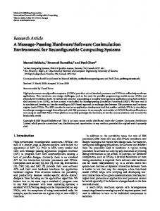
Our discussion to this point begs the question, what is the cost of this architecture? In order to quantify some of these costs, we performed a series of experiments, the results of which are shown in Figure 6. We found that while our architecture introduces a measurable increase in latency and decrease in throughput, these costs have a negligible impact when applied to a low bandwidth communications chan-

Building Block

Description

Status Command Packet Query Data Link

Reports current status, supports notification Accepts commands Forwards packet traffic with configurable queuing Serializes a queue of transactions Standard interface for network stack modules

Requires

Sensor Logring Directory

Buffered sensor data interface In-memory ring of log messages Defines mapping from string values to numbers

Table 1:

All Services and Tools HostMote, EmRun, TimeSync(2) HostMote, EmProxy DGH MoteNIC, UDP, LinkStats, Flooding, MoteSim(N) Audio Server(2), Weather Station(4), DGH(4) EmRun(N) TimeSync

Summary of Device Patterns, and the tools and services that use them.

280

udp-dev-linkstats+frag udp-dev-linkstats udp-dev udp-raw

Inter-Packet Send Time [msec]

0.2

udp-dev-linkstats+frag udp-dev-linkstats udp-dev udp-raw

1.2

0.15

0.1

0.05

270

1 260

0.8

Time(ms)

0.25

Inter-Packet Send Time [msec]

Used By

N/A N/A N/A Status Packet, Status, Command Status N/A Status

0.6 0.4

250

240

0.2 230

0

0 6

7

8

9 10 11 12 13 Log2 of Packet-Size [Bytes]

14

15

16

6

7

8

9 10 11 12 13 Log2 of Packet-Size [Bytes]

14

15

16

220

Motenic/No FUSD

Motenic

...+Linkstats

...+Frag

Figure 6:

Measuring the cost of the Em* stack. Graph (a) shows the results of our throughput test over loopback for raw UDP and three stack configurations. Graph (b) shows the results of our latency test. Graph (c) shows the results of the throughput test when run over the Mote radio.

nel. This is an important case, since Em* is designed for systems with an architecturally high ratio of CPU to communication. To characterize latency and throughput, we devised two tests. First, we performed a throughput test, in which a test application would send packets as quickly as possible over the channel. Second, we performed a latency test, in which a test application would send a series of “ping” messages over the channel, only sending the next “ping” upon receipt of the previous ping’s response. For both tests, the intersend time was recorded and analysed. All of our experiments were performed on a 900 MHz Pentium III running Linux 2.4.20, with no other users. For our first experiments, we wanted to select a channel that was fast and deterministic, to simplify accounting for the underlying channel costs in determining the cost of Em*. UDP over loopback seemed the ideal choice. For our baseline case, we wrote a simple UDP client and server that implemented both of our tests. The results of the throughput and latency tests for a variety of packet sizes over UDP are shown as the “udp-raw” curves in Figures 6(a) and 6(b). Next, we implemented an Em* version of the client and server, and ran the same tests on an Em* interface to the UDP loopback channel, shown as the “udp-dev” curves. The same communication occurred, only now it traversed the Em* Data Link interface (once in the throughput test, and four times in the latency test). We then added two additional layers to the Em* stack, and performed the tests again. The “udp-dev-linkstats” curves are results after adding the LinkStats service to the Em* stack; the “udpdev+ls+frag” curve are results from adding a Fragmenta-

tion service on top of LinkStats. We observe from the graphs that each additional layer adds a fixed amount of overhead, with a slight dependence on packet size. This corresponds well with previous measurements of FUSD suggesting that system call volume was the dominant factor in performance. An interesting observation is that the overhead of the lowest “udp-dev” layer is not constant, in fact decreasing with packet size. We don’t have a clear explanation for this, but speculate that it is related to scheduling delay in waking the client processes. We also observe that the ping latency is about 5x longer than the transmit latency. Since the ping consists of two traverses down the stack and two traverses up the stack, this suggests that traverses up the stack cost about 1.5x as much as traverses downwards. This could be explained by observing that traversing up requires a notification operation (triggering select()) followed by a read(), while traversing down requires only a write(). Figure 6(c) shows the result of the throughput test, using a Mote as the underlying channel instead of UDP, for 200 byte packets. Each bar shows the mean, plus or minus one standard deviation, for 1000 packet sends. The first bar shows the inter-send times achieved by integrating the HostMote serial protocol with the throughput test into a single process. The second bar shows the Em* MoteNIC/HostMote service layers, driven by our Em* throughput test application. The third bar tests with the Linkstats service layered above MoteNIC, and the fourth bar adds Fragmentation above Linkstats. In order to focus on the overhead of Em* interfaces (rather than protocol

overhead), the length of the payload issued at the top layer is adjusted in each case to generate 200 byte packets at the Mote radio layer. As we can see from the graph, the Em* layers do not have a significant impact on throughput. 3.3.3

Sensor Device

Two of the applications that drove the development of Em* centered around acquisition and processing of audio data. One application, a ranging and localization system [10], needed to extract and process audio clips from a specific time in the past. The other, a continuous frog call detection and localization system [17], needed to receive the data in a continuous stream. Both applications needed to be able to correlate time series data captured on a distributed set of nodes, thus timing relationships among the nodes needed to be maintained. The Sensor Device interface encapsulates a ring buffer that stores a history of sampled data, and integrates with the Em* Time Synch service to enable clients to relate local sensor data to sensor data from other nodes. A client of the sensor device can open the device and issue a request for a range of samples. When the sample data is captured, the client will be notified and the data will be streamed back to the client as it continues to arrive. Keeping a history of recent sensor data and being able to relate the sample timing across the network is critical to many sensor network applications. By retaining a history of sampled data, it is much easier to implement applications where an event detected on one node triggers further investigation and sensing at other nodes. Without local buffering, the variance in multi-hop communications times makes it difficult to abstract the triggered application from the communications stack.

3.4

Em* Events and Client APIs

One of the benefits of the Em* design is that services and applications are separate processes and communicate through POSIX system calls. As such, Em* clients and applications can be implemented in a wide variety of languages and styles. However, a large part of the convenience of Em* as a development environment comes from a set of helper libraries that improve the elegance and simplicity of building robust applications. In Section 3.2 we mentioned that an important part of device patterns is the library that implements them on the service side. Most device patterns also include a client-side “API” library, that provides basic utility functions, GLib compatible notification interfaces, and a crashproofing feature intended to prevent cascading failures. Crashproofing is intended to prevent the failure of a lower-level service from causing exceptions in clients that lead them to abort. It achieves this by encapsulating the mechanism required to open and configure the device, and automatically triggering that mechanism to automatically re-open the device whenever it closes unexpectedly. The algorithm used in crashproofing is described in Figure 7.

WATCH -C RASHPROOF(devname, CONFIG, HANDLER) 1 2 3 4 5 6 7 8 9 10 11 12 13 14 15 16 17 18 19

fd ← OPEN(devname) if CONFIGURE(fd) < 0 goto 11 crashed ← FALSE resultset ← POLL(fd, {input, except}) if crashed then status ← READ(fd, buffer ) if status < 0 abort if devname ∈ buffer goto 1 else if except ∈ resultset then CLOSE(fd) fd ← OPEN(“/dev/fusd/status′′ ) if fd < 0 abort crashed ← TRUE elseif input ∈ resultset then status ← READ(fd, buffer ) if fatal error goto 11 if status ≥ 0 HANDLER(buffer , status) goto 4

Figure 7:

“Crashproof” auto-reopen algorithm.

The arguments to this algorithm are the name of the device, and two callback functions, config and handler. The config function configures a freshly opened device file according to the needs of the client, e.g. setting queue lengths and filter parameters. The handler function is called when new data arrives. Note that in the implementation, the call to poll() occurs in the GLib event system, but the fundamental algorithm is the same. As a client, using crashproof devices is completely transparent. The client constructs a structure specifying the device name, a handler callback, and the client configuration, including desired queue lengths, filters, etc. Then, the client calls a constructor function that opens and configures the device, and starts watching it according to the algorithm in Figure 7. In the event of a crash and reopen, the information originally provided by the client will be used to reconfigure the new descriptor. The crashproof client libraries are supplied for both Packet and Status devices.

4

Examples

The last section enumerated a number of building blocks that are the foundation for the Em* environment. In this Section, we will describe how we have used them to construct several key Em* tools and services.

4.1

EmSim and EmCee

EmSim and EmCee are tools designed to simulate unmodified Em* systems at varying points on the continuum from simulation to deployment. EmSim is a pure simulation environment, in which many virtual nodes are run in parallel, interacting with a simulated environment and radio channel. EmCee is a slightly modified version of EmSim that provides an interface to real low-power radios in place of a simulated channel. EmSim itself is made up of modules. The main EmSim module maintains a central repository for node information, initially sourced from a configuration file, and exposed as a Status Device. EmSim then launches other mod-

ules that are responsible for implementing the simulated “world model” based on the node configuration. After the world is in place, EmSim begins the simulation, starting up and shutting down virtual nodes at the appropriate times. 4.1.1

Running Virtual Nodes

The uniform use of the /dev filesystem for all of our I/O and IPC leads to a very elegant mechanism for transparency between simulation, various levels of reality, and real deployments. The mechanism relies on name mangling to cause all references to /dev/* to be redirected deeper into the hierarchy, to /dev/sim/groupX/nodeY/*. This is achieved through two simple conventions. First, all Em* modules must include the call to misc init() early in their main() function. This function will check for certain environment variables to determine whether the module is running in “simulation mode”, and what its group and node IDs are. The second convention is to wrap every instance of a device file name with sim path(). This macro will perform name-mangling based on the information discovered in misc init().3 For simplicity, we typically include the sim path() wrapper at the definition of device names in interface header files. This approach enables easy and transparent simulation of many nodes on the same machine. This is not the case for many other network software implementations. Whenever the system being developed relies on mechanisms inside the kernel that can’t readily be partitioned into virtual machines, it will be difficult to implement a transparent simulation. For example, ad-hoc routing code that directly configures the network interfaces and kernel routing table is very difficult to simulate transparently. While a simulation environment such as NS-2 [24] does attempt to run much of the same algorithmic code as the real system, it does so in a very intrusive, #ifdef-heavy way. This makes it cumbersome to keep the live system in sync with the NS-2 version. In contrast, Em* modules don’t even need to be recompiled to switch from simulation to reality. In addition, the Em* device hierarchy interactively yields a great deal of transparency into the workings of each individual node. Of course, this flexibility brings a cost. An ad-hoc routing algorithm that dragged every packet to user-space would likely suffer poorer performance. 4.1.2

Simulated World Models

Given the capability to transparently redirect the IPC channels, we can provide a world for the simulated nodes to see, and in some cases, affect. There are many examples of network simulation environments in the networking community, some of which support radio channel modeling.[24][25] In addition, the robotics community has devoted much effort to creating world models.[16] For sensor networks, the robotic simulations are often more appropriate, because they are designed to model a system sens3 Thus,

misc init() must precede the use of sim path().

ing the environment, and intended to test and debug control systems and behaviors that must be reactive and resilient. The existence of Em* device patterns simplifies the construction of simulated devices, because all of the complexity of the interface behavior can be reused. Even more important, by using the same libraries, the chances of subtle behavior differences are reduced. Typically, a “simulation module” will read the node configuration from EmSim’s Status Device, and then expose perhaps hundreds of devices, one for each node. Requests to each exposed device will be processed according to a simulation of the effects of the environment, or in some cases in accordance with traces of real data. The notification channel in Em* status devices enables EmSim to easily support configurations changes during a simulation. Updates to the central node configuration, such as changes in the position of nodes, trigger notification in the simulation modules. The modules can then read the new configuration and update their models appropriately. In addition, we can close the loop by creating a simulation module that provides an actuation interface, for example enabling the node to move itself. In response to a request to move, this module could issue a command to EmSim to update that node’s position and notify all clients. 4.1.3

Using Real Channels in the Lab

EmCee is a variant of EmSim that integrates a set of virtual nodes to a set of real radio interfaces, positioned out in the world. We have two EmCee-compatible testbeds: the ceiling array and the portable array. The ceiling array is composed of 55 Crossbow Mica1 Motes, permanently attached to the ceiling of our lab in a 4 foot grid. Serial cabling runs back to two 32-port ethernet to serial multiplexers. The portable array is composed of 16 Crossbow Mica2 Motes and a 16-port serial multiplexer, that can be taken out to the field.[2] The serial multiplexers are configured to expose their serial port devices to appear to be normal serial devices on a Linux server (or laptop in the portable case). To support EmCee, the HostMote and MoteNIC services support an “EmCee mode” where they open a set of serial ports specified in a config file and expose their devices within the appropriate virtual node spaces. Thus, the difference between EmSim and EmCee is minimal. Where EmSim would start up a radio channel simulator to provide virtual radio link devices, EmCee starts up the MoteNIC service in “EmCee mode”, which creates real radio link devices which map to multiplexer serial ports and thus to real Motes. Our experience with EmCee has been well worth the infrastructure investment. Users have consistently observed that using real radios is substantially different than our best efforts at creating a modeled radio channel.[5][2] Even channels driven by empirical data captured using the ceiling array don’t seem to adequately capture the real dynamics. Although testing with EmCee is still not the same as

proves, as it becomes more likely that processes from the same simulated node will share a CPU. With this lesson in hand, subsequent versions of our simulator explicitly assign processes to CPUs, improving efficiency by keeping the highest-bandwidth communication within a CPU.

3

Normalized Aggregate Speed

2.5

4 CPUs 3 CPUs

2 2 CPUs 1.5

4.2 0.5

0 1

2

4

8 16 Number of Simulated Nodes

32

64

128

Figure 8: Performance of a simple EmSim simulation, varying the number of nodes simulated, and the number of CPUs available on the simulator platform. Each “node” is of a pair of processes that continuously exchange data via a FUSD Status Interface. We plot the aggregate transfer rate summed across all simulated nodes. Results are normalized so that y = 1 corresponds to the speed achieved by a single-node simulation (2 processes) running on a single CPU.

a real deployment, the reduction in effort relative to a deployment far outweighs the reduction in reality for a large part of the development and testing process. 4.1.4

EmRun

1 CPU

1

Performance of EmSim/EmCee

Currently, an important limitation of our simulator is that it can only run in real-time, using real timers and interrupts from the underlying operating system. This is unlike a discrete-event simulator such as ns-2, which runs in its own virtual time, so can run for as long as necessary to complete the simulation without affecting the results. The real-time nature of EmSim/EmCee makes performance an important consideration. With perfect efficiency, the simulator platform would need the aggregate computational power of all simulated nodes. To test the actual efficiency, we ran test simulations on a single SMP-enabled server with 4 700MHz Pentium-III processors, running Linux kernel 2.4.20. 4 In our initial testing, the default Linux scheduler was used; no explicit assignment of processes to CPUs was made. Each “node” consisted of two processes that continuously exchanged data via a FUSD Status Device. The results, shown in Figure 8, emphasize the need to run processes that intercommunicate heavily on a common CPU. A single-node simulation ran on a single-CPU platform at nearly at nearly twice the speed as on 2-, 3- or 4-CPU platform. The Linux scheduler’s default behavior of placing one process on each CPU is disastrously inefficient because those processes communicate with high bandwidth. A similar effect can be seen with the 2-node (4-process) simulation on a 4-CPU platform, which was slower than the 2CPU case where processes from a single “node” are forced onto the same CPU. The data also show that additional CPUs are beneficial if the processes are better partitioned. In the larger simulations, performance with larger numbers of CPUs im4 The number of CPUs available to the simulator was controlled using Andrew Morton’s “cpus allowed” patch.

EmRun starts up, maintains, and shuts down an Em* system according to the policy specified in a config file. There are three key points in its design: process respawn, inmemory logging, and fast startup, graceful shutdown. Respawn Process respawn is neither new, nor difficult to achieve, but it is very important to an Em* system. It is difficult to track down every bug, especially ones that occur very infrequently, such as a floating-point error processing an unusual set of data. Nonetheless, in a deployment, even infrequent crashes are still a problem. Often, process respawn is sufficient to work around the problem; eventually, the system will recover. In-Memory Logs EmRun saves each process’ output to in-memory logrings that are available interactively from the /dev/emlog/* hierarchy. These illustrates the power of FUSD devices relative to traditional logfiles. Unlike rotating logs, Em* logrings never need to be switched, never grow beyond a maximum size, and always contain only recent data. Fast Startup EmRun’s fast startup and graceful shutdown is critical for a system that needs to duty cycle to conserve energy. The implementation depends on a control channel that Em* services establish back to EmRun when they start up. Em* services notify EmRun when their initialization is complete and are ready to respond to requests. The emrun init() library function, called by the service, communicates with EmRun by writing a message to /dev/emrun/.int/control. EmRun then launches other processes waiting for that service, based on a configured dependency graph. This feedback enables EmRun to start independent processes with maximal parallelism, and to wait exactly as long as it needs to wait before starting dependent processes. This scheme is far superior to the naive approach of waiting between daemon starts for pre-determined times, i.e., the ubiquitous “sleep 2” statements found in *NIX boot scripts. Various factors can make startup times difficult to predict and high in variance, such as flash filesystem garbage collection. On each boot, a static sleep value will either be too long, causing slow startup, or too short, causing services to fail when their prerequisites are not yet available. Graceful Shutdown The control channel is also critical to supporting graceful shutdown. EmRun can send a message through that channel, requesting that the service shut down, saving state if needed. EmRun then waits for SIGCHLD to indicate that the service has terminated. If the process is unresponsive, it will be killed by a signal.

1 13

Beamforming

14

2

AudioServer

3 4 5 6

15

6

7

9

8

10 11

12 7

EmProxy

TimeSync

8 9

4

10 5

Neighbors

11

Flooding

12 13 14

2

3

15

LinkStats

16 17

1

16 17

EthernetLink

N

EmRun

18

18 N

Link device /dev/link/udp0/data Link device /dev/link/stats0/data Status device /dev/link/stats0/stats Status device /dev/link/stats0/neighbors Link device /dev/routing/flood/data Status device /dev/sync/params/ticker Command dev /dev/sync/params/command Status device /dev/sync/client/pulses Command dev /dev/sync/client/command Status device /dev/sync/pairs/pulses Command dev /dev/sync/pairs/command Directory dev /dev/sync/clock-types Sensor dev /dev/audio/0/buffered Packet dev /dev/audio/0/sync Status dev /dev/emproxy/clients Status dev /dev/emrun/status Command dev /dev/emrun/command FUSD dev /dev/emrun/.int/control Logring devs /dev/emlog/*

Figure 9: Block diagram of an Em* system, showing the types of interfaces and linkages. The boxes in gray are all standard Em* services, while the white box is an notional application, similar to one implemented against an earlier version of Em* components[4]. Note that all services have a control channel to EmRun, although only four are shown (dashed arcs). An interesting property of the EmRun control channel is one that differentiates FUSD from other approaches. When proxying system calls to a service, FUSD includes the PID, UID, and GID of the client along with the marshalled system call. This means that EmRun can implictly match up the client connections on the control channel to the child processes it has spawned, and reject connections from nonchild processes. This property is not yet used much in Em* but it provides an interesting vector for customizing device behavior.

4.3

Time-Synchronized Sampling in Em*

Several of the driving applications for Em* have involved distributed processing of high-rate audio: audible acoustic ranging, acoustic beamforming, and animal call detection are a few of the applications. We used earlier versions of Em* to tackle a few of these problems[17][4][10]; the current version of Em* includes support for these types of application. In this section, we will describe the services that enable this in more detail. Figure 9 shows a block diagram of a time-synchronized sampling system. The TimeSync service and the AudioServer service collaborate to enable an application such as a Beamformer to acquire time series and relate them to time series from other nodes across the network. TimeSync Between Nodes The TimeSync service uses Reference Broadcast Synchronization (RBS)[7] to compute relationships among the CPU clocks on nodes in a given broadcast domain. This technique correlates the arrival times of broadcast packets at different nodes, and uses linear regression to estimate conversion parameters among clocks that receive broadcasts in common. We chose RBS because techniques based on measuring send times, such as TPSN[9], are not generally applicable without support at the MAC layer. Requiring this support would rule out many possible radios, including 802.11 cards. A key insight in RBS is that it is better to enable conversion than to attempt to train a clock to follow some remote “master” clock. Training a clock has many negative repercussions for the design of a sampling system caused

by clock discontinuities and distortions. Thus, TimeSync is really a “time conversion” service. The output of the regression is reported through the /dev/sync/params/ticker device, in a complete listing of all known pairwise conversions. Clients of TimeSync read this device to get the latest conversion parameters, then convert times from one timebase to another. The code for reading the device and converting among clocks is implemented in a library. TimeSync within a Node Many systems have more than one clock. For example, a Stargate board, with an attached Mote and an audio card has three independent clocks. Thus to compare audio time series from two independent nodes, an index in a time series must be converted first to local CPU time, then to remote CPU time, and finally to a remote audio sample index. The TimeSync service provides an interface for other services to supply pair-wise observations to it, i.e. a CPU timestamp and a clock-X timestamp. This interface uses a Directory device to enable clients to create a new clock, and associate it with a numeric identifier. The client then writes periodic observations of that clock to the timesync command device /dev/sync/params/command. The observations are fit using linear regression to compute a relationship between the two local clocks. The Audio Server The Audio service provides a Sensor Device output5 . It defines a “sample clock”, which is the index of samples in a stream, and submits observations relating the sample clock to the CPU time to TimeSync. A client of the Audio service can extract a sequence of data from a specific time period by first using TimeSync to convert the begin and end times to sample indices and then placing a request to the Audio service for that sample range. Conversely, a feature detected in the streaming output at a particular sample offset can be converted to a CPU time. These clock relations can also be used to compute and correct the skew in sample rates between devices, which can otherwise cause significant problems. 5 Actually,

it was the model for the Sensor Device pattern.

Generating the synch observations requires minor changes to the audio driver in the kernel. We have made patches for two audio drivers: the iPAQ built-in audio driver and the Crystal cs4281. In both cases, incoming DMA interrupts are timestamped and retrieved by the Audio service via ioctl(). While this approach makes the system harder to port to new platforms and hardware, it is a better solution for building sensing platforms. The more common solution, the “synchronized start” feature of many sound cards, has numerous drawbacks. First, it only give you one data point for the run, where our technique gives you a continous stream of points to average. Second, it is subject to drift, and since the end is not timestamped there is no way to accurately determine the actual sample rate. Third, it forces the system to coordinate use of the audio hardware, whereas the Audio server runs continuously and allows access by multiple clients.

5

Design Philosophy and Aesthetics

In this section, we will describe some of the ideas behind the choices we made in the design of Em*.

5.1

No Local/Remote Transparency

One of the disadvantages of FUSD relative to sockets is that connections to FUSD services are always local, whereas sockets provide transparency between local and remote connections. Nonetheless, we elected to base Em* on FUSD because we felt that the advantages outweighed the disadvantages. The primary reason for giving up remote transparency in Em* is that remote access is never transparent in wireless sensor networks. WSNs are characterized by communications links that have high or variable latency, have varying link quality and evolving topologies, and generally low bandwidth. In addition, because communication has a significant energy cost, WSNs strive to develop innovative protocols that minimize communications, make use of broadcast channels, tolerate high latency, and enable tradeoffs to be made explicit to the system designer. Not only is remote communication in WSNs demonstrably different than local communication, very little is achieved by masking that fact. In abandoning remote transparency, the client gains the benefit of knowing that each synchronous call will be received and processed by the server with low latency. While an improperly implemented server can introduce delays, there is never a need to worry that a network problem might introduce an unexpected delay. Requests that are known to be time consuming can be explicitly implemented so that the results are returned asynchronously via notification (e.g. Query Device).

5.2

Intra-Node Fault Tolerance

Tolerance of node failures (or the failure of intervening communications networks) is an important part of the design of distributed systems. In the case of embedded sys-

tems, several issues conspire to make node robustness a high priority. First, the cost of responding to node failure can be much higher for embedded systems. This is especially true if network access to the node is unreliable and a physical journey is required; in extreme cases, nodes may be physically irretrievable. Second, many applications of WSNs are aimed at discovering new properties of their environment that could not previously be studied. By its nature, this task exposes the system to new inputs that may in turn exercise new bugs. We apply several techniques to address fault tolerance within a node: EmRun respawn, “crashproofing”, soft-state refresh, and transactional interface design. We discussed EmRun respawn and crashproofing in Sections 4.2 and 3.4, as means of keeping the Em* services running, and preventing cascading failures when an underlying service fails. Soft-state and transactional design are key ideas in the design of many distributed services, and are equally applicable within an Em* node. Status devices are typically used in a soft-state mode. Rather than reporting “diffs”, every status update reports the complete current state, leaving the client to decide how to respond based on its own state. While this approach is less efficient, when the update rate is low it’s usually easy to make the case for trading efficiency for robustness and simplicity. Similarly, periodic refreshes in the absence of notification are often used to limit the damage caused by a missing notification signal. In the other direction, state pushed by a client to a service typically uses a transactional approach with soft-state refresh, for similar reasons. Rather than admitting the possibility that the client and server are out of synch (e.g. in the event of a server restart), the client periodically resubmits its complete state to the service, enabling the service to make appropriate corrections if there is a discrepancy. Where the state in question is very large, there may be reason to implement a more complex scheme, but for small amounts of state simplicity and robustness carry the day.

5.3

Code Reuse

Code reuse and support for modularity were major design goals of Em*. Despite being written in a nonOOP language, Em* manages to achieve a high degree of reusabililty through disciplined design, as can be seen in Table 2. Em* has largely been designed by factoring useful components from existing implementations. In this way, we guarantee at least one user for each library. The device patterns have all arisen in this way; they exemplify solutions that apply to a useful class of problems. Em* services have been designed following the dictum “encapsulate mechanism, not policy”. By extracting the mechanism from the application but leaving the policy, we can reduce the complexity of the system while maintaining simple interfaces between independent processes. While the approach of packaging mechanism in libraries can yield a similar simplicity of interface, in that case the application is still at the mercy of bugs or unexpected interactions be-

tween its code and the library code. With Em* that complexity is offloaded to a separate process, whose fate the application does not share. Building Block Status Device and derivatives Command Device Packet Device Data Link Interface

Table 2:

5.4

Server Uses

Client Uses

40 17 10 12

22 N/A 5 32

Reuse statistics culled from LXR.

Reactivity

Reactivity one of the most interesting characteristics of WSNs. They must react to hard-to-predict changes in their environment in order to operate as designed. Often the tasks themselves require a reaction, for example a distributed control system or a distributed sensing application that triggers other sensing activities. Em* is designed to support reactivity through the notification interfaces in Em* devices. Em* also encourages services and applications to be written in an event-driven style that lends itself to reactive design. Many Em* services are written in a style that decouples the “input” and “output” call chains, with shared state in the middle. Thus, the input side makes changes to the state, and notifies the output side to recompute. Independently, the output side processes the current state according to its own schedule and the needs of clients. This design can greatly simplify implementation given the many possible orders of event arrival.

5.5

High Visibility

While the decision to stress visibility in the Em* design was partly motivated by aesthetics, it has paid off handsomely in overall ease of use, development, and debugging. The ability to browse the IPC interfaces in the shell, to see human-readable outputs of internal state, and in many cases to manually trigger actions makes for very convenient development of a system that could otherwise be quite cumbersome. Tools like EmView also benefit greatly from stack transparency, because EmView can snoop on traffic travelling in the middle of the stack in real time, without modifying the stack itself.

6

Conclusion and Future Work

In conclusion, we have found Em* to be a very useful development environment for WSNs. We are using Em* at CENS as the basis for a 50-node seismic deployment that is currently under development, as well as for numerous local development projects. We are also directing resources to supporting other groups with their Em* based projects, including the NIMS project and the ISI ILENSE group. We are currently focusing on Em* support for the Crossbow/Intel Stargate platform, which is an inexpensive Linux platform based on the XScale processor. Compared with the iPAQ platforms we had used previously, Stargates are much easier to modify and much easier to buy.

We are also planning several Em* extensions. To support high-bandwidth sensor interfaces such as high-rate audio, image data, and signal processing modules, we plan to add a shared-memory based data channel to Sensor device. We also plan to implement a device proxy that can enable remote access to devices over local high-speed interconnects, for example to allow cpus in same logical system to share devices. Through work on the NIMS project, we hope to gain more experience with sensors, actuators, and simulated world-models.

References [1] In Proc. of the First Intl. Conf. on Embedded Networked Sensor Systems (ACM Sensys), Los Angeles, CA, Nov. 2003. [2] A. Cerpa, N. Busek, and D. Estrin. SCALE: A tool for Simple Connectivity Assessment in Lossy Environments. Technical report, CENS-TR-21, September 2003. [3] A. Cerpa, J. Elson, D. Estrin, L. Girod, M. Hamilton, and J. Zhao. Habitat Monitoring: Application Driver for Wireless Communications Technology. In 2001 ACM SIGCOMM Workshop on Data Communications in Latin America and the Caribbean, San Jose, Costa Rica, Apr. 2001. [4] J. Chen, L. Yip, J. Elson, H. Wang, D. Maniezzo, R. Hudson, K. Yao, and D. Estrin. Coherent Acoustic Array Processing and Localization on Wireless Sensor Networks. Proceedings of the IEEE, 91(8), August 2003. [5] H. Dubois-Ferriere. Using voronoi clusters to scope floods from multiple sinks. Talk given at CENS Systems Seminar, Oct. 2003. [6] J. Elson, S. Bien, N. Busek, V. Bychkovskiy, A. Cerpa, D. Ganesan, L. Girod, B. Greenstein, T. Schoellhammer, T. Stathopoulos, and D. Estrin. EmStar: An Environment for Developing Wireless Embedded Systems Software. Technical report, CENS-TR-9, March 2003. [7] J. Elson, L. Girod, and D. Estrin. Fine–grained network time synchronization using reference broadcasts. In OSDI, pages 147–163, Boston, MA, December 2002. [8] D. Estrin, W. Michener, G. Bonito, and W. Participants. Environmental Cyberinfrastructure Needs for Distributed Sensor Networks: A Report From an NSF Workshop. Workshop Report, Scripps Institute of Oceanography, La Jolla, CA, Aug. 2003. [9] S. Ganeriwal, R. Kumar, and M. Srivastava. Timing Sync Protocol for Sensor Networks. In Sensys, 2003. [10] L. Girod, V. Bychkovskiy, J. Elson, and D. Estrin. Locating tiny sensors in time and space: a case study. In In ICCD 2002, Freiburg, Germany, September 2002. http://lecs.cs.ucla.edu/Publications. [11] J. Heidemann, F. Silva, and D. Estrin. Matching Data Dissemination Algorithms to Application Requirements. In Sensys, 2003. [12] J. Hill, R. Szewczyk, A. Woo, S. Hollar, D. Culler, and K. Pister. System Architecture Directions for Networked Sensors. In ASPLOS 2000, Cambridge, USA, Nov. 2000. [13] C. Intanagonwiwat, R. Govindan, and D. Estrin. Directed Diffusion: A Scalable and Robust Communication Paradigm for Sensor Networks. In In MobiCom 2000, Boston, USA, Aug. 2000. [14] P. Levis, N. Lee, M. Welsh, and D. Culler. TOSSIM: Accurate and Scalable Simulations of Entire TinyOS Applications. In Sensys, 2003. [15] A. Mainwaring, J. Polastre, R. Szewczyk, D. Culler, and J. Anderson. Wireless Sensor Networks for Habitat Monitoring. In WSNA, number 1, 2002. [16] R. T. Vaughan, B. Gerkey, and A. Howard. On Device Abstractions For Portable, Resuable Robot Code. In In IEEE/RSJ IROS 2003, Las Vegas, USA, October 2003. [17] H. Wang, J. Elson, L. Girod, D. Estrin, and K. Yao. Target Classification and Localization in Habitat Monitoring. In In ICASSP 2003, Hong Kong, China, April 2003. [18] H. Wang, D. Estrin, and L. Girod. Preprocessing in a Tiered Sensor Network for Habitat Monitoring. In in EURASIP JASP Special Issue on Sensor Networks, number 4, pages 392–401, 2003. [19] W. Ye, J. Heidemann, and D. Estrin. An energy-efficient MAC protocol for wireless sensor networks. In Proceedings of IEEE INFOCOM, 2002. [20] Center for embedded networked sensing. http://www.cens.ucla.edu. [21] Crossbow mica2. http://www.xbow.com. [22] Gnu hurd. http://www.gnu.org/software/hurd/docs.html. [23] James reserve. http://cens.ucla.edu/Research/Applications. [24] Ns-2. http://www.isi.edu/nsnam/ns/ns-documentation.html. [25] Parsec. http://pcl.cs.ucla.edu/projects/parsec/manual. [26] Qnx. http://www.qnx.com.