Embedded-Particle Computation in Evolved Cellular Automata

Extended abstract In T. Toffoli, M Biafore, and J. Leao (eds.), Physics and Computation ’96 (Pre-proceedings), New England Complex Systems Institute, 153-158, 1996.

Embedded-Particle Computation in Evolved Cellular Automata Wim Hordijk James P. Crutchfield∗ Melanie Mitchell ∗

1

Introduction

the neighborhood’s central cell at the next time step. In a one-dimensional CA, a neighborhood consists of a cell and its radius r neighbors on either side.

In our work we are studying how genetic algorithms (GAs) can evolve cellular automata (CAs) to perform computations that require global coordination. The “evolving cellular automata” framework is an idealized means for studying how evolution (natural or computational) can create systems that perform emergent computation, in which the actions of simple components with local information and communication give rise to coordinated global information processing [3].

One-dimensional binary-state cellular automata are perhaps the simplest examples of decentralized, spatially extended systems in which emergent computation can be observed. In our studies, a CA performing a computation means that the input to the computation is encoded as the IC, the output is decoded from the configuration reached at some later time step, and the intermediate steps that transform the input to the output are taken as the steps in the computation.

In previous work [4, 5], we analyzed the process by which a genetic algorithm designed CAs to perform particular tasks. In this paper we focus on how these CAs implement the emergent computational strategies for performing a task. In particular, we develop a class of embedded-particle models to describe the computational strategies implemented by particular CAs. To do this, we use the computational mechanics framework of Crutchfield and Hanson [2, 6], in which a CA’s information processing is described in terms of regular domains, embedded particles, and their interactions. We then evaluate this class of models by comparing their computational performance to that of the CAs they model. The results demonstrate, via a generally close quantitative agreement between the CAs and the embedded particle models, that this new model class captures the significant functional features in the CAs’ space-time behavior that underlie the CAs’ computational capability and evolutionary fitness.

2

Santa Fe Institute, Santa Fe, NM and Physics Department, University of California, Berkeley

To date, we have used a genetic algorithm (GA) to evolve one-dimensional, binary-state r = 3 CAs to perform a density-classification task [3, 4] and a synchronization task [5]. For the density classification task, the goal is to find a CA that decides whether or not the IC contains a majority of 1s (i.e., has high density). More precisely, we call this task the “ρc = 1/2” task. Here ρ denotes the density of 1s in a binary-state CA configuration and ρc denotes a “critical” or threshold density for classification. Let ρ0 denote the density of 1s in the IC. If ρ0 > ρc , then within M time steps the CA should reach the fixed-point configuration of all 1s (i.e., all cells in state 1 for all subsequent iterations); otherwise, within M time steps it should reach the fixed-point configuration of all 0s. M is a parameter of the task that depends on the lattice size N . For the synchronization task, the goal is to find a CA that, from any IC, settles down within M time steps to a periodic oscillation between an all-0s configuration and an all-1s configuration. Again, M is a parameter of the task that depends on N .

CAs and Computation

This paper concerns one-dimensional binary-state CAs with periodic (circular) boundary conditions. Such a CA consists of a one-dimensional lattice of N two-state machines (“cells”), each of which changes its state as a function only of the current states in a local neighborhood.

Since the CA can only use local interactions, and thus has to propagate information across the lattice to achieve global coordination, both tasks require a nontrivial computation by the CA. For example, in the synchronization task, the entire lattice has to be synchronized, which means the CA must, using only local interactions, resolve separate regions of the lattice that are locally synchronized but are out of phase with respect to one another.

The lattice starts out with an initial configuration (IC) of cell states (0s and 1s) and this configuration changes at discrete time steps during which all cells are updated simultaneously according to the CA’s rule φ. A CA’s rule φ can be expressed as a lookup table that lists, for each local neighborhood, the state which is taken on by 1

3

Analysis of Evolved CAs

0

Time

Due to the local nature of a CA’s operations, it is typically very hard, if not impossible, to understand the CA’s global behavior—in our case, the strategy for performing a computational task—by directly examining either the bits in the lookup table or the temporal sequence of raw 0-1 spatial configurations of the lattice. Crutchfield and Hanson developed a method for detecting and analyzing the “intrinsic” computational components in the CA’s space-time behavior in terms of regular domains, particles, and particle interactions [2, 6]. This method is part of their computational mechanics framework for understanding information processing embedded in physical systems [1]. Briefly, a regular domain is a homogeneous region of space-time in which the same “pattern” appears. More formally, the spatial patterns in a regular domain can be described by a regular language that is mapped onto itself by the CA rule φ. An embedded particle is a spatially localized, temporally recurrent structure found at domain boundaries, i.e., where the domain pattern breaks down. When two or more particles “collide” they can produce an interaction result—e.g., another set of particles or a mutual annihilation.

74

0

Site

74

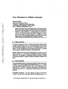
Figure 1: Space-time diagram of a GA-evolved CA φsync1 with measured performance 1.0 on the synchronization task. After [5].

Using computational mechanics, we can analyze the space-time behavior of evolved CAs in terms of these domains, particles, and interactions. Fig. 1 shows a spacetime diagram of φsync1 —a CA that was evolved for the synchronization task—starting with a randomly generated IC. (Cells in state 1 are colored black, cells in state 0 are colored white. Time increases down the page.) We define the performance PN,I (φ) of a CA φ on a given task as the fraction of I randomly generated ICs on which φ reaches the desired behavior within M time steps on a lattice of length N . For the synchronization task, we let M = 2.15N and we measured PN,104 (φsync1 ) to be 1.0 for N = 149, 599, 999.

α

Time

β δ

γ

β ν

µ γ

In φsync1 ’s space-time behavior, there are two regular domains: the “synchronized” domain (the parts of the lattice which display the desired oscillation) and a second domain which looks like a zigzag pattern. (These regions are readily apparent in Fig. 1.) Having identified these domains, we can build a filter that removes them, revealing the domain boundaries, which in this case are predominantly particles. The filtered space-time diagram is shown in Fig. 2, where the regular domains are mapped to 0s (white), and the domain boundaries are mapped to 1s (black).

0

Site

γ

δ

74

Figure 2: Filtered version of space-time diagram in Fig. 1. Domains are mapped to white, particles to black. The different particle types are labeled with Greek letters. After [5].

which its spatial configuration repeats. The velocity of a particle is the number of sites it is shifted in space after exactly one temporal period, divided by the temporal periodicity. For example, the particle µ in Fig. 2 has a temporal periodicity of 2, and after 2 time steps it has shifted 6 sites in space, so its velocity is 3.

A catalog of φsync1 ’s observed particles and their properties (temporal periodicity and velocity), and all possible particle interactions, is given in Table 1. The temporal periodicity of a particle is the number of time steps after

As was mentioned earlier, we consider the embedded 2

ing embedded-particle model employs a number of simplifying assumptions.

φsync1 Particles Label Temporal Velocity Prob. at tc Periodicity α 0 0.00 β 2 1 0.39 γ 2 -1 0.40 δ 4 -3 0.07 µ 2 3 0.07 ν 2 -1 0.07 φsync1 Interactions α → γ + β, γ + δ → ∅, µ + β → ∅ β + γ → δ + µ (0.84), β + γ → ν (0.16) µ + ν → γ, µ + δ → γ + β, ν + δ → β

Define the condensation time tc as the first time step at which the lattice can be completely described in terms of domains and particles. The occurrence of the condensation time is illustrated in Fig. 3 for a GA-evolved CA, φsync2 , that has lower performance on the synchronization task than φsync1 . The condensation time (tc = 28 in this particular case) is marked by the solid line. It is the time step at which the “random” structure at the center of the lattice has died out and there remain only domains and particles. As can be seen in Fig. 3, at later time steps after the condensation time, “random” structures (neither domains nor particles) can occur again as a consequence of a particle interaction. We will ignore this in the model (see the fourth assumption below), and define tc as the first time step at which the lattice contains only domains and particles.

Table 1: A catalog of φsync1 ’s particles and their properties, and interactions, some of which can be observed in the filtered space-time diagram of Fig. 2. An interaction result denoted by ∅ means that the two particles annihilate. The probabilities associated with the occurrence of particles at tc and with their interactions (in parentheses) are given. If no explicit probability is given for an interaction, the interaction result occurs with probability 1.0. These particle and interaction probabilities are explained in section 4. For φsync1 , tc was measured to be 26.

The particular value of tc for a given CA depends on the IC, but we can estimate the average condensation time tc for a given rule by sampling tc over a large set of random ICs. The measured value of tc for various rules will be used later when we test the models. For φsync2 , tc was measured to be 49.

particles to be the main behavioral components supporting the CA’s emergent computation. Particles transfer information about a property of a local region across the lattice to distant sites. Particle collisions are the loci of information processing and result in either the creation of new information in the form of other particles or in annihilation. Our claim is that this particle-level description captures the mechanisms by which the CA is capable of transferring and processing local information to accomplish global coordination.

4

0

tc Time

A Formal Model of Computational Strategies

Interestingly, the high-performance CAs found in both the density classification and synchronization task GA runs all exhibited domains, particles, and particle interactions. Moreover, although these components differed in details in different CAs, they were all used to implement variations of a general strategy consisting of competition between regions of similar density or local synchronization phase. The largest regions eventually dominate the lattice and so determine the final configurations. In this sense, there is a common computational strategy for performing the tasks.

99 0

Site

99

Figure 3: Space-time diagram of a lower-performance evolved CA, φsync2 , for the synchronization task, starting with a randomly generated IC. The condensation time tc = 28 is marked by the solid line.

As a first simplifying assumption of the model, we replace the spatio-temporal dynamics that can be observed up to the condensation time by a particle probability distribution at tc . In this, we assume that the net effect of the dynamics up until tc is to generate some distribution of particles of various types, randomly located in

To formalize the notion of computational strategy in a CA, we model the CA’s behavior using only the notions of domains, particles, and interactions. The result3

the lattice at that time, and that beyond generating this distribution, the initial “pre-condensation” dynamics are not relevant to estimating the average performance. We estimate this particle probability distribution empirically over a set of randomly generated ICs to obtain the occurrence frequency of each particle type at tc . For example, the empirical distribution for the particles of φsync1 is given in Table 1, measured over 104 ICs.

together with the probability that each particular result occurs. These probabilities can be estimated empirically by simply counting, over a set of random ICs, how often each interaction result occurs in the space-time diagram. In the model, when two particles collide, the table is consulted and an interaction result is determined at random according to these probabilities. For example, in Table 1, the β + γ interaction has two possible outcomes. Each is given with its estimated probability of occurrence.

Actually, this particle distribution depends on the total number of particles that occur at tc . Since the lattice has periodic boundary conditions, the domain (or particle) in which site N − 1 participates must agree with the domain (or particle) that site 0 contributes to. Given a total number of particles in the lattice, certain particles have to occur more often than other particles in order to obey these constraints. For example, some particle types must always occur in pairs. The embedded-particle model therefore uses a probability distribution for the total number of particles occurring at tc , together with a particle probability distribution conditioned on this total number of particles. It uses both distributions to generate a particle configuration at tc .

In summary, the embedded-particle model of a CA’s computational strategy consists of: 1. A catalog of possible particle types, their probabilities, and their associated domains. 2. A probability distribution of pure domain-particle configurations at tc . 3. A set of pairwise particle interactions and results, along with the interaction-result probabilities for each. These components are given in Table 1 for φsync1 .

Furthermore, since the correct final configuration of the CA (all black or all white) for the density classification task depends on the density of the initial configuration, we split up the particle probability distribution for CAs for this task in a distribution generated by low density ICs (ρ0 < 0.5) and a distribution generated by high density ICs (ρ0 > 0.5).

5

Testing the Embedded-Particle Model

One way to test a model is to compare its performance to that of the actual CA. If the model can predict the CA’s performance PN,I (φ), this will support our claim that the embedded-particle model is a good description of the CA’s computational strategy. This is a quantitative complement to the computational mechanics analysis which establishes the structural role of domains, particles, and interactions.

As a second simplifying assumption, in the model all particles have zero width, even though, as can be seen in Fig. 3, particles actually have varying widths. As a third simplifying assumption, we allow interactions only between pairs of particles. No interactions involving more than two particles are included in the model.

To run the model, we start by generating an initial particle configuration at tc , according to the particle probability distribution in the model. This simply puts a number of particles of various types in the lattice at random locations, uniformly distributed over the lattice. Thus at tc we know for each particle its type, and thus its velocity, and its spatial location. (The value tc in the model is assigned the measured value of tc for the CA.)

A fourth simplifying assumption we make is that particle interactions are instantaneous. As can be seen in Fig. 3, when two particles collide and interact with each other, typically the interaction takes time to occur—for some number of time steps the lattice cannot be completely described in terms of domains and particles. In the embedded-particle model when two particles collide they are immediately replaced by the interaction result.

It is then straightforward to calculate geometrically at what time step t the first interaction between two particles will occur (i.e., the time step at which two particles will collide). The table with interaction-result probabilities is consulted, and the result of this particular interaction is determined. The two interacting particles are then replaced by the interaction result, yielding a new particle configuration at time step t. This overall process is iterated either until there are no particles left in the lattice (they all annihilated) or until a given maximum number (M − tc ) of time steps is reached, whichever occurs first.

In a CA’s space-time behavior, the interaction result is determined by the phases that both particles are in at the time of their collision. As a fifth simplifying assumption, we approximate an interaction’s relative phase dependence by a stochastic choice of phase. To determine an interaction result, the model uses a table (similar to Table 1), containing interaction-result probabilities. For each possible pair of particle types, this table lists all the interaction results that these two particles can produce, 4

We refer to this iteration process as the “ballistic particle dynamics” of the model. (See Fig. 4.)

CA Model

1 0.9 0.8

MODEL

tc

0.7

- Particles

Performance

Time

- Domains - Interactions Space

0.6 0.5 0.4 0.3

M

0.2

Figure 4: Schematic illustration of running the embeddedparticle model. An initial particle configuration at tc is generated first. Then the ballistic particle dynamics is iterated for a maximum number (M − tc ) of time steps.

0.1 0

φsync2

φdens1

φdens2

Figure 5: Comparison of the average performances (labeled “CA”) and the model-estimated average performances (labeled “Model”) for four different evolved CA.

Since the embedded-particle model contains information about which domains form which particles, we can keep track of the domains between the particles at each time step while the model is run. Thus, if all particles eventually annihilate each other, we know which domain is left occupying the entire lattice.

6

φsync1

As both Fig. 5 and Table 2 show, there is very close agreement between the average CA and model performances for both the synchronization rule φsync2 and the density rule φdens1 , with only 1% and 3% difference respectively.

Results

For φsync1 the discrepancy between the average CA and model performances is about 5%. This discrepancy is caused by the temporal periodicity of four of the “zigzag” domain (see Fig. 1). Because of the periodic boundary conditions, on a lattice size of 149 the real CA can never settle down to a configuration containing only the zigzag domain. However, this can happen in the embeddedparticle model, since it ignores the spatial periodicity of domains. Such configurations count as incorrect behavior and the model yields a slightly lower performance for φsync1 .

We can now estimate the performance of a particular CA by running its model on a large number of ICs and calculating the fraction over which it displays the correct behavior (i.e., settles down to the correct domain within the maximum number of allowed time steps). Fig. 5 shows the results of comparing the average performances of four different evolved CAs with the estimated average performances produced by running the embedded-particle models of their respective strategies. In all cases the average performance is calculated over 10 sets of 104 random ICs (in case of the actual CAs) or initial particle configurations (in case of the models), with N = 149 and M = 2.15N . Table 2 gives the average performances (with standard deviations given in parentheses).

There is a discrepancy of about 23% for φdens2 . This can be explained by the fact that, for φdens2 , the distances between the particles at tc are important characteristics. These distances—ignored by the model—reflect the sizes of the domains that are in between the particles and are key in φdens2 ’s strategy. Since the model distributes the particles randomly over the lattice, this leads to a lower model performance for φdens2 . This is less of a problem for φdens1 , since its strategy is much less dependent on these inter-particle distances.

The first two CAs, φsync1 and φsync2 , are GA-evolved rules for the synchronization task. φsync1 is the best rule found for this task; its strategy is shown in Fig. 1. φsync2 is a rule that appeared early on in the GA run, and so it still has relatively low performance; its strategy is shown in Fig. 3.

The generally good agreement between the performance of a model and that of the corresponding CA demonstrates the promise of the embedded-particle model. The discrepancies noted above, which can be explained, demonstrate where our simplifying assumptions fail. We expect to be able to improve on the model’s agreement

The next two rules, φdens1 and φdens2 , are GA-evolved rules for the density classification task. Both rules appeared later on in the GA run, and φdens2 was the best CA found for this task. 5

Rule φsync1 FEB1C6EA B8E0C4DA

P149,104 (φ) CA Model 1.0000 0.9519 (0.0000)

(0.0032)

0.1799

0.1823

(0.0034)

(0.0039)

Difference 5%

tc 26

1%

49

and under NSF grant IRI-9320200 and DOE grant DEFG03-94ER25231. It was supported by the University of California, Berkeley, under ONR grant N00014-95-1-0524.

6484A5AA F410C8A0

φsync2 CEB2EF28 C68D2A04

References

38

[1] Crutchfield, J. P., “The calculi of emergence: Computation, dynamics, and induction”, Physica D 75 (1994), 11–54.

16

[2] Crutchfield, J. P., and J. E. Hanson, “Turbulent pattern bases for cellular automata”, Physica D 69 (1993), 279–301.

E341FAE2 E7187AE8

φdens1 05004581 00000FBF6

0.6923

0.6675

(0.0039)

(0.0035)

3%

B9F75937 FBDF77F

φdens2 05040587 05000F770

0.7701

0.5904

(0.0037)

(0.0049)

23%

[3] Crutchfield, J. P., and M. Mitchell, “The evolution of emergent computation”, Proceedings of the National Academy of Sciences, USA 92 (23) (1995), 10742–10746.

37755837 BFFB77F

Table 2: Comparison of the CA average performances and the embedded-particle model average performances for four different evolved CA rules. These averages are calculated over 10 sets of 104 ICs each. The standard deviations are given in parentheses. The tc used for each model is given, as is the hexadecimal code for each CA’s φ, with the most significant bit being associated with the neighborhood 0000000.

[4] Das, R., M. Mitchell, and J. P. Crutchfield, “A genetic algorithm discovers particle-based computation in cellular automata”, Parallel Problem Solving from Nature—PPSN III (Y. Davidor, H.-P. Schwefel, and ¨ nner, eds.) (1994), 244–353. R. Ma [5] Das, R., J. P. Crutchfield, M. Mitchell, and J. E. Hanson, “Evolving globally synchronized cellular automata”, Proceedings of the Sixth International Conference on Genetic Algorithms, (L. Eshelman ed.), (1995), 336–343.

with these and other CAs by incorporating a few additional features, such as the domain-size distribution. Preliminary results support the validity of these expectations.

7

[6] Hanson, J. E., and J. P. Crutchfield, “The attractorbasin portrait of a cellular automaton”, Journal of Statistical Physics 66 (5/6) (1992), 1415–1462.

Conclusions

Emergent computation in decentralized spatially extended systems, in particular in CAs, is still not well understood. In previous work we have used an evolutionary approach to search for CAs that are capable of performing computations that require global coordination, and have qualitatively analyzed the emergent “computational strategies” in terms of domains, particles, and particle interactions. The embedded-particle models described in this paper provide a means to more rigorously formalize the notion of “emergent computational strategy” in spatially extended systems and to make predictions about their behavior and their evolutionary fitness. This is an essential, quantitative part of our overall research program—to understand how natural spatially extended systems can perform globally coordinated computations and how evolutionary processes can give rise to systems with sophisticated emergent computational abilities.

Acknowledgments This research was supported by the Santa Fe Institute, under the Adaptive Computation and External Faculty Programs (supported by ONR grant N00014-95-1-0975) 6