Title: Embedded system for real time flight flutter detection Authors: Tadeusz Uhl, Maciej Petko, Bart Peeters, Herman Van der Auweraer
In Proceedings of the 6th International Workshop on Structural Health Monitoring, Stanford University, CA, USA, 11-13 September 2007
ABSTRACT The paper presents an idea of flutter margin detection algorithm which is based on identification of natural frequencies and modal damping ratio for airplane structure employing in-flight vibration measurements. The method is based on application of wavelets filtering for decomposition of measured system response into components related to particular vibration modes. In the second step classical Recursive Least Square (RLS) estimation methods is used to obtain ARMA model parameters. The hardware implementation of proposed algorithm is based on FPGA technology which allows implementing complex algorithm in a one chip. The results of modal parameters tracking using designed real-time embedded system are compared with more classical in-flight modal analysis at discrete flight points. . INTRODUCTION Unstable vibrations of an airplane can be a reason of a catastrophic failure of the aircraft [1]. In the literature [2], [3], [4] many cases of flutter phenomena are carefully studied. The procedure of in-flight flutter testing consists of measurements of structural vibration of an airplane and, based on these measurements, an estimation of modal model parameters [5], [6]. Each possible aircraft configuration should be tested separately. Many papers are focused on development of operational modal analysis methods which can be directly applied for modal parameters estimation during a flight [7], [8]. Some are realized iteratively in real time, with less than 1 second interval between estimations [9]. During the proposed procedure; based on recorded signals, the modal parameters of the structure are estimated using any identification method. The procedure should be applied at each test point to determine Flight Clearance Envelope (FCE) [4]. There are many different modal parameters identification methods that could be used for flight flutter testing [8]. Both time domain and frequency domain methods match the requirements for on-line modal parameters identification [9]. The time-domain method, based on classical recursive RLS algorithm, is applied as the proposed solution and is efficient enough and relatively easy to implement. The idea of the proposed method is based on application of Tadeusz Uhl, Maciej Petko, AGH University of Science and Technology, al. Mickiewicza 30, 30-059 Krakow, Poland, e-mail:
[email protected] Bart Peeters, Herman Van der Auweraer, LMS International, Interleuvenlaan 68, 3001 Leuven, Belgium
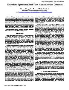
wavelets filtering for decomposition of measured system response into components related to particular vibration modes [10, 11]. These components can be extracted in parallel way for all modes. The procedure can be applied to any number of measured signals and consists of steps listed in the diagram (Fig. 1).
Figure 1. Diagram of applied flutter margin detection procedure
In the second step classical Recursive Least Square (RLS) estimation methods is used to obtain ARMA model parameters. The second order model is assumed in implementation to obtain modal parameters for separated modes. The limitations of implementation are amount of FPGA resources (for parallel wavelet transformation engines and signals and wavelets buffers) and computational speed (for sequential calculations of RLS and estimation of modal parameters). During estimation phase confidence bounds are calculated to assess quality of the procedure. There are different methods for confidence bounds estimation in modal analysis techniques [11, 15], but only a few can be realized on-line. The method implemented in the formulated procedure is based on the linearization of the relation between the ARMA model parameters variance and the standard deviation of the modal parameters. A METHOD OF FLUTTER MARGIN ESTIMATION The time domain method is formulated for linear systems with time-varying parameters. The model parameters are estimated for each time step of the iteration based on values from a previous calculation. The recursive identification methods are widely used in adaptive control systems [16]. The flowchart of the recursive procedure for damping estimation is depicted in figure 3. Parameters estimators are computed at each sampling interval according to the minimum of objective function which is defined as follows:
[ ]
i
[
V θˆ(i ) = ∑ α i − j y ( j ) − ϕ T ( j − 1)θ (i ) j =1
]
2
(1)
where: α is the forgetting factor, which describes the influence of the j-th sample on the i-th estimator, 0 < α ≤1. If the model parameters are not changing, α should be set
as 1. The proper choice of the α (which oscillate between 0.95 and 0.99) value gives better parameters tracking properties of the algorithm. Accelerometers and analog signal conditioning Many modes
Analog signal A/D Converter
Time series Wavelets based filter Selected modes
Estimation of ARMA model parameters
DAMPING ESTIMATION
i=i+1
NATURAL FREQUENCY ESTIMATION
Modal damping
Natural frequency
Figure 2. Flowchart of recursive method for damping estimation.
The basic assumption for the algorithm is that covariance matrix P is positive definite at each iteration step: def
P −1 (i ) =
i
∑α
i− j
ϕ ( j − 1)ϕ T ( j − 1)
(2)
j =1
The ARMA model’s parameters in the presented method are estimated from the iterative formula: θ (i + 1) = θ (i) + K (i)( y (i + 1) − φ (i + 1) T θ (i )) K (i ) = P(i + 1)φ (i + 1) (3)
P(i + 1) = ( I − K (i )φ (i + 1) T ) P(i ) In order to find the damping ratio for given vibration natural mode, poles of the system should be found. The second order model is assumed for each analyzed mode and many independent models can be investigated concurrently. It simplifies the process of system poles extraction. The ARMA model represents discrete model of the system but to assess values of modal parameters the poles of continues system are required The relationship between continues and discrete poles are as follows [17]: 1 δj = ln(λ j λ*j ) (4) 2T Ωj =
Im(λ j ) 1 arctg 2T Re(λ j )
j = 1, 2, ..., 2n − 1
(5)
where; λi is the characteristic polynomial root for discrete case, δ i , Ωi are the damping ratio and natural frequency for continuous case, T is the sampling period.
ASSESSMENT OF CONFIDENCE BOUNDS FOR FLUTTER MARGIN REAL TIME ESTIMATORS
During recursive identification, covariance matrix elements P(i) are estimated at each step of the procedure. Diagonal parameters of the covariance matrix are variances of the particular ARMA model parameters [16]. These parameters are inputs of confidence bounds estimation for modal parameters for all modes under investigation. The relationship between the ARMA model parameters and the modal model parameters is strongly nonlinear because the ARMA model is defined in the discrete time domain (sampled signal) but the modal parameters are identified in the continuous time domain. To find the confidence bound based on known ARMA parameters the variance linearization of relation between the ARMA and the modal parameters has to be linearized [15]. The Taylor expansion method is proposed for this purpose. The covariance matrix for modal parameters can be estimated at each step of the procedure by applying the following formula:
[
]
T T T Pˆκ (κˆ n ) = J (θˆN )E (θ 0 − θˆN )(θ 0 − θˆN ) J (θˆN ) = J (θˆN )Pθ (θˆn )J (θˆN )
(6)
where: κˆn is the vector of the modal parameters at sample n, J() is the Jacobian matrix, θˆN is a vector of the ARMA model parameters, θ 0 is the vector of exact value of the
ARMA model parameters, P(θn) is the covariance matrix of the ARMA model parameters, Pk(κn) is the covariance matrix of the modal parameters. The Jacobian matrix can be obtained from the numerical differentiation using the central difference theorem. The i-th column of matrix J (θ N ) can be numerically estimated by:
(
) (
f θˆNH + dθ i − f θˆNH − dθ i J i θˆNH = 2dθ i
( )
)
(7)
where; dθi is a small ARMA parameter perturbation of the value one order of the magnitude smaller than the required accuracy of standard deviation estimation; f is a function expressing the relationship between the modal parameters and parameters of the ARMA model (equations (4) and (5)). The standard deviation of modal parameters can be numerically calculated, according to equations (6) and (7), from the diagonal elements of matrix Pκ(κn). IMPLEMENTATION ALGORITHM
OF
THE
FLUTTER
MARGIN
MONITORING
Performance of calculations depends on how fast and how precisely individual parts of the algorithms are realized. Increased precision means longer time needed for calculations. Imposed tight execution time restrictions can be satisfied using a fast, expensive processor, a multiprocessor system or by mixed hardware-software implementation. The latter option was selected so as to allow for the greatest flexibility, future improvements and modifications. All calculations are shared
between software (dark gray blocks) and hardware (light gray blocks), as shown in Fig. 3, on a system created on a Stratix FPGA chip. Software means that parts of the algorithm are written in C and then compiled for a Nios II soft-processor. Hardware fragments are realized in the logic of the FPGA and the Avalon Bus is used for data exchange. The flutter margin monitoring algorithm consists of five steps (Fig. 3): data read from the analog-to-digital converters (ADC), convolution of a stored wavelet with signals from sensors, signals reconstruction, on-line recursive least square (RLS) routine for estimation of parameters of the ARMA models, and determination of damping coefficients for flutter detection. The floating-point operations of the software part are accelerated by custom instructions created in the Nios II ALU hardware, namely, floating-point addition, multiplication, reciprocal and square root. Data acquisition from the DACs is performed with a programmable frequency in the range of 10-200 Hz.
Figure 3. Hardware-software partitioning of the flutter monitoring algorithm
The RLS algorithm and damping coefficients calculations are performed for each wavelet-filtered signal in the floating-point arithmetic by the processor being supported by custom instructions. The flutter appearance can then be determined using the damping coefficients thresholds table indexed by the actual flight conditions. VERIFICATION OF THE DESIGNED FLUTTEROMETER
The performance of the flutterometer has been verified on acceleration signals recorded with a sampling frequency of 160 Hz during flight test of a TS-11 Iskra military jet aircraft that performed at variable speeds within the 250-750 km/h range. During the flutterometer verification experiment, two signals were used: one measured a fin and the second the tail of the plane. At both points, two modes of vibration dominate: the first with a frequency of 27 Hz and the second 47 Hz. They were decoupled by convolution of 512 signal samples with Morlet wavelets around
100 points long. Convolution of such lengths of signals and wavelets buffers with signal reconstruction takes 2.5 ms per sample, irrespective of the number of modes analyzed. Recursive RLS algorithm damping ratio calculations consume 0.5 ms of processor time per sample per mode. All calculations for the four modes take 4.5 ms per sample and results in over 200 Hz of maximum sampling frequency.
Figure 4. Estimated on-line natural frequency and modal damping with their confidence intervals.
Thus, processing 20 modes would take 12.5 ms, allowing for signals sampling with 80 Hz. Assuming the confidence level to be 99.7%, uncertainty bounds for the modal parameters estimated using the procedure described in section 3, are shown in figure 4. As it can be noticed in the figure 4, the confidence bounds for the system under analysis are relatively small, but only at the start of the recursion process variability of parameters have an unacceptable level. COMPARISON WITH CLASSICAL IN-FLIGHT MODAL ANALYSIS AT DISCRETE FLIGHT POINTS
The same data was also analyzed in a classical way using non-recursive algorithms. In this paper, the Operational Modal Analysis version of PolyMAX was used [18]. The main advantage of PolyMAX is that it yields extremely clear stabilization diagrams. This makes an automation of the parameter identification process rather straightforward and enables a continuous monitoring of the dynamic properties of a structure [19]. The idea adopted here was to use a so-called “sliding window” approach. The time data was split in highly-overlapping segments and each segment was processed independently and automatically. The chosen segment length was 1600 samples. The segments were overlapping 95%, which mean that every 0.5 s an update of the modal parameters is available. These modal parameters are of course not the instantaneous modal parameters, but are assumed to be “representative” for the whole processed segment of 10 s. Fig.5 shows the automatic processing results of a single segment. The PolyMAX settings were; Block size of the autocorrelation function = 256 samples (number of time lags), Exponential window parameter = 1%, Frequency band 20 – 60 Hz, Maximum model order = 20. These settings allowed a very quick calculation (less than 0.5s) of the modal parameters. The good correspondence between measured and synthesized spectrum confirms that the analysis was successful (see figure 5 – Right). In the figure 5, the automatic PolyMAX results of all data segments are represented. An automated mode tracking procedure was applied to these results. The outcome of the tracking operation is represented in Figure 6. Two
tail sensors 7 and 8 have been processed independently with the described procedure. The frequency values estimated from both sensors agree very well (Figure ). Although the damping ratios show a larger variance, again both sensors agree well. Moreover, the trends in the damping ratios correspond very well to the online results presented in the figure 4. o
s s s s s v s s v s
18 16
Model order
14 12 10
v v v v o
8 6
s s s s s s s s s s
s s s s s s s s s v
s s s v o o
s s s v o
o v o
Measured Synthesized
Power spectrum
20
2
10
4 2 0 20
25
30
35
40 f [Hz]
45
50
55
60
20
25
30
35
40 f [Hz]
45
50
55
60
Figure 5: (Left) PolyMAX stabilization diagram + automatic selection of poles. (Right) correspondence between measured and synthesized spectrum. Mode 1 Frequency Tracking
Mode 1 Damping Ratio Tracking
28
1.2 Sensor 7 Sensor 8
0.8 Damping ratio [%]
27.6 Frequency [Hz]
Sensor 7 Sensor 8
1
27.8
27.4
27.2
0.6
0.4
0.2 27
0 26.8 10
20
30
40
50 t [s]
60
70
80
90
-0.2 10
20
30
40
50 t [s]
60
70
80
90
Figure 6. Tracking of the eigenfrequency at 27 Hz. Data from 2 sensors was processed independently (left). Tracking of the damping ratio of the mode at 27 Hz. Data from 2 sensors was processed independently (right).
CONCLUSIONS
A formulated algorithm allows computing modal parameters of complex structures on-line during a flight. Implementation of the flutter monitoring algorithm is proposed with the Hardware-Software Co-design approach, i.e. a part realized by hardware and the remaining part by software running on a Nios II soft-processor contained in the FPGA. The flutterometer is an example of the System-on-Chip, which allows for high level of integration and flexibility – it can be altered, e.g. to optimize for different algorithms, or to add some functionality, by reprogramming the FPGA without modifications of the PCB. For the tested structure, 12 first modes parameters have been identified simultaneously during 0.001 second. Confidence intervals for all parameters are relatively small and the method can be applied for flight flutter testing based on in-flight measurements. As it was shown the results are very similar to results obtained using different classical methods realized off- line.
ACKNOWLEDGEMENTS
This work was carried out in the frame of the EUREKA project E! 3341 FLITE2. The financial support of the Institute for the Promotion of Innovation by Science and Technology in Flanders (IWT) is gratefully acknowledged. Polish partners have been financed by the Ministry of Science and Higher Education within a frame of Eureka Flite2 project. REFERENCES [1] [2] [3] [4] [5] [6] [7] [8] [9] [10] [11] [12] [13] [14] [15] [16] [17] [18] [19]
M.W. Kehoe: A historical Preview of flight flutter testing, AGARD Conference Proceedings 566, Advanced Aeroservoelastic Testing and Data Analysis, (1995). I.E. Garrick and W.H. Reed: Historical development of aircraft flutter, Journal of Aircraft, v.18, (1981), pp. 897-912. M.J. Brenner, R.C. Lind and D.F. Voracek: Overview of recent flight flutter testing research at NASA Dryden, NASA TM/4792, (1997). A.A. Abbasi and J.E. Cooper: Current Status and Challenges for Flight Flutter Testing, Proceedings of ISMA 2006 Conference, Leuven, (2006), pp. 1523- 1546. E. Nissim and G.B. Gilyard: Methods for Experimental determination of flutter speed by parameter Identification, NASA TP-2923, (1989). G. Dimitriadis and J.E. Cooper: Flutter prediction flight flutter test data, AIAA Journal of Aircraft, vol. 38, (2001), pp. 355-367,. L. Hermans and H. Van der Auweraer: Modal testing and analysis of structures under operational conditions: Industrial applications, Mechanical Systems and Signal Processing (1999) 13(2), pp. 193-216. T. Uhl, W. Lisowski and P. Kurowski: In-operation modal analysis and its application, AGH, Krakow, (2001). M. Bogacz and T. Uhl: Real time modal model identification and its application for damage detection, Proceedings of ISMA 2004 Conference, Leuven, (2004), pp. 1065- 1075. A. Klepka and T. Uhl: Application of wavelet transform to identification of modal parameters of nonstationary systems, J. of Theoretical and Applied Mech., Vol. 43, (2005) ,pp. 277-296. A. Klepka: Identification of modal parameters of mechanical structures in nonstationary conditions, PhD thesis, AGH Univ. of Science and Technology, Krakow, (2005) (in Polish). T. Kambe, A. Yamada and M. Yamaguchi: Trend of system level design and approach to Cbased design, Microelectronics Journal, Vol. 33, (2002), pp. 875-880. M. Petko and G. Karpiel: Semi-Automatic Implementation of Control Algorithms in ASIC/FPGA, in 2003 IEEE Conference on Emerging Technologies and Factory Automation: Proceedings, vol. 1, pp. 427-433. M.D. Edwards, J. Forrest and A.E. Whelan: Acceleration of software algorithms using hardware/software co-design techniques, J. of Systems and Architecture, Vol. 42, (1996/97), pp. 697-707. P. Andersen, Identification of Civil Engineering structures using Vector ARMA Models, Ph D. Thesis, Aalborg University, 1997 Söderström, T., P., Stoica (1988), System identification, Prentice-Hall Int., Hempstead, U.K. T. Uhl., Computer assisted identification of mechanical structures,(in Polish), WNT, Warszawa, 1998 J. Lau, J. Lanslots, B. Peeters, H. Van der Auweraer. Automatic modal analysis: reality or myth? In Pro. of IMAC 25, the International Modal Analysis Conference, Orlando (FL), USA, 19-22 February 2007. B. Peeters, H. Van der Auweraer, F. Vanhollebeke, P. Guillaume. Operational modal analysis for estimating the dynamic properties of a stadium structure during a football game. Shock and Vibration – Special Issue: Assembly Structures under Crowd-Dynamic Excitation, Accepted for publication, 2007