Center for Neural Science, and ... We present an embedded image coder based on a statistical .... efficients at adjacent spatial locations (which we call âsib-.
Presented at:
4th IEEE International Conference on Image Processing, Santa Barbara, CA. October 26-29, 1997. c IEEE 1997.
Embedded Wavelet Image Compression Based on a Joint Probability Model Eero P. Simoncelli
Robert W. Buccigrossi
Center for Neural Science, and Courant Inst. for Mathematical Sciences New York University New York, NY 10003
GRASP Laboratory Computer and Information Science Dept. University of Pennsylvania Philadelphia, PA 19104
We present an embedded image coder based on a statistical characterization of natural images in the wavelet transform domain. We describe the joint distribution between pairs of coefficients at adjacent spatial locations, orientations, and scales. Although the raw coefficients are nearly uncorrelated, their magnitudes are highly correlated. A linear magnitude predictor, coupled with both multiplicative and additive uncertainties, provides a reasonable description of the conditional probability densities. We use this model to construct an image coder called EPWIC (Embedded Predictive Wavelet Image Coder), in which subband coefficients are encoded one bit-plane at a time using a non-adaptive arithmetic encoder. Bit-planes are ordered using a greedy algorithm that considers the MSE reduction per encoded bit. We demonstrate the quality of the statistical characterization by comparing ratedistortion curves of the coder to several standard coders. The popularity of the World Wide Web and the development of large image databases have created a demand for flexible embedded image representations. Orthonormal wavelet pyramids, in which images are decomposed using basis functions localized in spatial position, orientation, and spatial frequency (scale), have proven to be extremely effective for image compression. We believe there are several statistical reasons for this success. The most widely known of these is that wavelet transforms are reasonable approximations to the Karhunen-Lo`eve expansion for fractal signals [1], such as natural images [2]. The resulting redistribution of variance leads to a reduction in the total entropy of the wavelet coefficients relative to the entropy of the original image pixels.
First-order Model In addition to redistributing variance, wavelet transforms produce coefficients with significantly non-Gaussian marginal statistics [e.g., 3, 4, 5, 6]. This observation should be contrasted with frequency-based decompositions, which produce marginals that are much closer to Gaussian. Since the Gaussian is the maximal-entropy density for a given variance, EPS is supported by NSF CAREER grant MIP-9796040, and the Sloan Center for Theoretical Neurobiology at NYU. RWB is supported by NSF Graduate Fellowship GER93-55018.
wavelet-based coders can achieve higher degrees of compression than frequency-based coders such as JPEG. Figure 1 shows histograms of a horizontal wavelet subband for several images. Compared to a Gaussian, these densities are more sharply peaked at zero, with more extensive tails. To quantify this, we give the sample kurtosis (fourth moment divided by squared second moment) below each histogram. The estimated kurtoses of all of the subbands are significantly larger than the value of three expected for a Gaussian distribution. Also shown in the figure are two-parameter model density functions of the form [3, 6]: P
(c)
/
e,jc=sj : p
(1)
The density parameters fs; pg are chosen by minimizing the relative entropy (also known as the “Kullback-Leibler divergence”) between a discretized model distribution and the 256bin coefficient histogram. We make no claim of uniqueness or optimality here: for example, Zhu et. al. used a different class of density functions to characterize these statistics [7]. Note that by describing the statistics in this simplistic fashion, we are assuming both independence and stationarity of the subband coefficients, both of which are generally incorrect. We will continue to assume stationarity, but we address the independence issue next.
Joint Model The coefficients of wavelet subbands are nearly uncorrelated. Nevertheless, casual inspection illustrates that wavelet coefficients are not statistically independent. Specifically, largemagnitude coefficients tend to occur at the same relative locations in subbands at adjacent scales [8]. Such dependencies have been utilized implicitly in a number of image compression schemes. Shapiro [9] developed the Embedded Zerotree Wavelet (EZW) coder, which takes advantage of the observation that a zero coefficient of a subband is likely to indicate a tree of zero coefficients at the same location in all finer scale subbands. Several authors [10, 11, 12] have used vectorized lookup tables to predict blocks of fine coefficients from blocks of coarse coefficients. Schwartz et. al. [13] used adaptive entropy coding to capture conditional statistics of coefficients based on the most significant bits of each of
Lena
CTscan
Toys
log(probability)
Boats
−100
−50
� = 14:5;
0
50
100
�H = 0:079
−100
−50
� = 18:9;
0
50
100
−100
�H = 0:067
−50
� = 22:9;
0
50
100
�H = 0:25
−100
−50
� = 23:0;
0
50
100
�H = 0:076
Figure 1. Examples of 256-bin coefficient histograms (solid lines) for vertical bands of four images, plotted in the log domain. Also shown (dashed lines) are fitted densities corresponding to equation (1). Below each histogram is the sample kurtosis (fourth moment divided by squared variance), and the relative entropy. The CTscan histogram was the worst fit (in terms of relative entropy) in our image set. the eight spatial neighbors and the coefficient at a coarser scale. Said and Pearlman [14] used a predictive scheme to give high-quality zerotree coding results. Chrysafis and Ortega [15] switched between multiple probability models depending on values of neighboring coefficients, and Wu and Chen [16] have extended the EZW coder to use local coefficient “contexts”.
the magnitudes Qk of eight adjacent coefficients in the same subband, two coefficients at other orientations, and a coefficient at a coarser scale. The linear combination is chosen to be optimal in a least-squares sense. The distribution has a similar appearance to the single-parent distribution of figure 2A. But the linear region is extended, and the conditional variance is significantly reduced.
We wish to characterize these statistical relationships explicitly. Consider two coefficients representing horizontal information at adjacent scales, but the same spatial location. Figure 2A shows the log-domain conditional histogram H 2 C j 2 P , where P is the magnitude of the coarse-scale (“parent”) coefficient and C is the magnitude of the finer-scale (“child”) coefficient. Observe that the right side of the distribution is unimodal and concentrated about a unit-slope line, indicating that C is roughly proportional to P . Furthermore, vertical cross sections (i.e., the histogram conditioned on a fixed value of P ) have roughly the same shape for different values of P . The left side of the distribution is concentrated about a horizontal line, suggesting that C is independent of P in this region. We suspect that these low-amplitude coefficients are dominated by quantization and other “noise” sources.
In order to determine which coefficients to include in the conditioning set fQk g, we calculated the mutual information be~ for a variety of choices of interband and intween C and l Q traband coefficients. Rather than exhaustively explore all possible neighbor subsets, we used a greedy algorithm to choose the five conditioning neighbors yielding the largest reduction in entropy.
( )
(log ( ) log ( ))
The fact that the conditional histograms seem to have a constant shape that shifts linearly with the predictor in the log domain suggests a model of multiplicative uncertainty. In particular, we use the following model for the conditional density:
~ ) + N; C 0 = M � l(Q
(2)
=
( )
0 ~ is where C 0 is the signed coefficient (i.e., C jC j), l Q the linear magnitude predictor described previously, and M and N are two mutually independent zero-mean random variables. Note that C 0 will be uncorrelated with each of the conditioning coefficients, Qk .
The form of the histogram shown in figure 2A is surprisingly robust across a wide range of images. We have used this statistical relationship between adjacent-scale coefficients in a previous coder implementation [8]. In the current paper, we incorporate a further observation: the qualitative form of these joint statistical relationships also holds for pairs of coefficients at adjacent spatial locations (which we call “siblings”), adjacent orientations (“cousins”), and adjacent orientations at a coarser scale (“aunts”).
The distribution of M is empirically determined. We constructed a lookup table for the conditional cumulative distribution in the log domain by averaging the mean- and variance-normalized conditional histograms of three training images (Lena, Boats, Baboon), at two scales (levels 2 and 3) and all three orientations. We assume N is independent of M , and Gaussian distributed. The fwk g are chosen to be leastsquare optimal, and the variances of M (in the log domain) and N are chosen to minimize the relative entropy between the joint model density and the joint histogram. Figure 2C shows the model density that best fits the density of figure 2B.
Given the linear relationship between large-amplitude coefficients and the difficulty of characterizing the density of a coefficient conditioned on its neighbors, we decided to examine a linear predictor for coefficient magnitude. Figure 2B shows a conditional histogram for C given a linear combination of 2
A
B
4
log2(C)
2
2
log (C)
3
1
6
6
5
5
4
4
3
3
log 2(C)
5
C
2 1
2 1
0
0
0
−1
−1
−2
−2
−1 −2 −3 −4
−2
0 log (P)
2
4
−2
2
0 2 4 log2(Linear Predictor)
6
−2
0 log 2(l(Q))
2
4
6
Figure 2. Conditional histograms of a coefficient in a horizontal subband of the “Boats” image. Intensity corresponds to probability, except that each column has been independently rescaled to fill the full range of intensities. A: Conditioned on a coefficient in a coarser-scale horizontal subband. B: Conditioned on an linear combination of coefficient magnitudes from adjacent spatial positions, orientations, and scales. C: Model of equation (2) fitted to the conditional histogram in B.
Coder Implementation and Results 6
We have implemented two versions of an image compression algorithm called EPWIC (Embedded Predictive Wavelet Image Coder). Both coders are based on a separable QMF decomposition using 9-tap symmetric (linear phase) filters [17]. Convolution boundaries are handled by symmetric reflection of the image about the edge pixels. EPWIC-1 uses the twoparameter first-order probability model of equation (1) to describe each subband. EPWIC-2 uses the joint linear predictive model of equation (2). We use a non-adaptive arithmetic coder to encode coefficients one bit-plane at a time. The coder uses the probability model to determine the probability of each bit being non-zero, conditioned on the bits already sent. The receiver uses the model to compute a conditional mean estimate for the coefficients, given the bits received thus far.
Entropy (bits/coeff)
5
4
3
2 First Order Ideal Conditional Model 1 1
2
3 4 5 Ideal Conditional Entropy
6
Bit-planes are ordered using a greedy algorithm which determines the bit-plane with the largest MSE reduction per encoded bit. The sign of each coefficient is sent only when needed (immediately after the first non-zero magnitude bit) as in [13]. Lowpass coefficient bit-planes are run-length encoded. The encoded bitstreams include an identification tag (2 bytes), the image width and height (2 bytes each), the number of pyramid levels (1 byte), quantization binsizes (2 bytes/subband), and the model parameters (9 bytes/subband), and bit-plane identification tags (1 byte/bit-plane). Full details may be found in [18].
Figure 3. Comparison of encoding cost using the conditional probability model of equation (2), and the encoding cost using the first-order histograms, as a function of the encoding cost using a � -bin joint histogram. Points are plotted for 6 bands (2 scales, 3 orientations) of the 13 images in our sample set.
256 256
An entropy calculation shows the value and quality of the model. Figure 3 shows a scatterplot comparing encoding cost based on the joint probability model of equation (2) vs. the encoding cost assuming accurate knowledge of a � bin histogram. Also included is a comparison to the encoding cost using the first-order histograms of figure 1. The conditional model typically falls short of the ideal by less than 0.5 bit/coefficient, but typically outperforms the first-order model by more than 0.5 bit/coefficient.
Figure 4 shows a rate-distortion comparison of several coders, averaged over 13 example images. Included are the JPEG coder1 , the EZW coder2 [9], EPWIC-1, and EPWIC-2. The example image set includes several landscapes, several faces, texture images, two medical images, and a synthetic image.
256 256
1 Independent JPEG Group’s CJPEG, version 5b. 2 We thank the David Sarnoff Research Center for their assistance in the
EZW comparisons.
3
60
1.5
Relative SNR (dB)
Relative Encoding Size (%)
EPWIC−2
1 0.5
EPWIC−1 0 EZW
−0.5 JPEG
−1 −1.5 −2 0.25
1
4 Kilobytes
16
50 40
JPEG
30 20 EZW
10 0
EPWIC−1
−10
EPWIC−2 25
64
30 SNR(dB)
35
Figure 4. Relative rate-distortion tradeoff for four image coders (JPEG, EZW, EPWIC-1, and EPWIC-2). Left: PSNR values (in dB), relative to EPWIC-1 (dotted horizontal line), as a function of the number of encoded bytes. Right: Number of bytes necessary to achieve a given PSNR, relative to EPWIC-1 (dotted horizontal line). All curves are averages over the set of images (of size � ) in our collection.
13
512 512
EPWIC-1 outperforms EZW for most compression ratios by about 0.3dB, and EPWIC-2 outperforms EZW by 0.5dB at 1Kbyte, and nearly 1.5dB at 16Kbytes and above. Also shown in figure 4 is the encoding size (relative to that of EPWIC-1) as a function of target PSNR. This gives a sense of how long one would wait during a progressive transmission for an image of a given quality. For example, EZW would have a transmission time roughly 30% higher than EPWIC-2 for an image quality of 25dB.
[7] S Zhu, Y Wu, and D Mumford. Filters, random fields and maximum entropy (FRAME) – towards the unified theory for texture modeling. In IEEE Conf. Computer Vision and Patt Rec, June 1996. [8] R W Buccigrossi and E P Simoncelli. Progressive wavelet image coding based on a conditional probability model. In ICASSP, Munich, Germany, April 1997. [9] Jerome Shapiro. Embedded image coding using zerotrees of wavelet coefficients. IEEE Trans Sig Proc, 41(12):3445–3462, December 1993. [10] A P Pentland, E P Simoncelli, and T Stephenson. Fractal-based image compression and interpolation, 1992. U.S. Patent Number 5,148,497, filed 2/14/90, issued 9/15/92. [11] A Pentland and B Horowitz. A practical approach to fractalbased image compression. In A B Watson, editor, Digital Images and Human Vision. MIT Press, 1993. [12] R Rinaldo and G Calvagno. Image coding by block prediction of multiresolution subimages. IEEE Trans Im Proc, July 1995. [13] E Schwartz, A Zandi, and M Boliek. Implementation of compression with reversible embedded wavelets. In Proc SPIE, 1995. [14] A Said and W A Pearlman. An image multiresolution representation for lossless and lossy compression. IEEE Trans. Image Proc, 5(9), September 1996. [15] C Chrysafis and A Ortega. Efficient context-based entropy coding for lossy wavelet image coding. In Data Compression Conference, Snowbird, Utah, March 1997. [16] X Wu and J Chen. Context modeling and entropy coding of wavelet coefficients for image compression. In ICASSP, Munich, April 1997. [17] E P Simoncelli and E H Adelson. Subband transforms. In John W. Woods, editor, Subband Image Coding, chapter 4. Kluwer Academic Publishers, Norwell, MA, 1990. [18] R W Buccigrossi and E P Simoncelli. Image compression via joint statistical characterization in the wavelet domain. Technical Report 414, GRASP Laboratory, University of Pennsylvania, May 1997. Available at ftp://ftp.cis.upenn.edu/pub/eero/buccigrossi97.ps.gz.
We have presented a statistical model for images in the wavelet transform domain, and have demonstrated the power of the model by using it explicitly in an image coder implementation. The compression results are quite good, especially given the simplicity of the encoding scheme and the fact that we did not utilize the statistical properties of the coefficient signs. The model should prove useful in other wavelet-based applications, such as image enhancement and texture synthesis.
References [1] G Wornell. Wavelet-based representations for the 1=f family of fractal processes. Proc. IEEE, September 1993. [2] D L Ruderman and W Bialek. Statistics of natural images: Scaling in the woods. Phys Rev. Letters, 73(6), August 1994. [3] S G Mallat. A theory for multiresolution signal decomposition: The wavelet representation. IEEE Pat. Anal. Mach. Intell., 11:674–693, July 1989. [4] D J Field. What is the goal of sensory coding? Neural Computation, 6:559–601, 1994. [5] B A Olshausen and D J Field. Natural image statistics and efficient coding. Network: Computation in Neural Systems, 7:333–339, 1996. [6] E P Simoncelli and E H Adelson. Noise removal via bayesian wavelet coring. In Third Int’l Conf Im Proc, pages 379–383, Lausanne, Switzerland, September 1996.
4