1516
J. Opt. Soc. Am. A / Vol. 24, No. 6 / June 2007
Urban et al.
Embedding non-Euclidean color spaces into Euclidean color spaces with minimal isometric disagreement Philipp Urban, Mitchell R. Rosen, and Roy S. Berns Munsell Color Science Laboratory, Chester F. Carlson Center for Imaging Science, Rochester Institute of Technology, 54 Lomb Memorial Drive, Rochester, New York 14623, USA
Dierk Schleicher School of Engineering and Science, International University Bremen, Postfach 750 561, D-28725 Bremen, Germany Received October 31, 2006; revised January 22, 2007; accepted January 23, 2007; posted January 29, 2007 (Doc. ID 76586); published May 9, 2007 Isometric embedding of non-Euclidean color spaces into Euclidean color spaces is investigated. Owing to regions of nonzero Gaussian curvature within common non-Euclidean color spaces, we focus on the determination of transformations into Euclidean spaces with minimal isometric disagreement. A computational method is presented for deriving such a color space transformation by means of a multigrid optimization, resulting in a simple color look-up table. The multigrid optimization is applied on the CIELAB space with the CMC, CIE94, and CIEDE2000 formulas. The mean disagreement between distances calculated by these formulas and Euclidean distances within the new spaces is far below 3% for all investigated color difference formulas. Color space transformations containing the inverse transformations are provided as MATLAB scripts at the first author’s website. © 2007 Optical Society of America OCIS codes: 330.0330, 330.1730.
1. INTRODUCTION A color space in which Euclidean distances agree with perceptual distances is of high importance in many image processing applications, such as color engineering, color image compression (due to optimal perceptual quantization), and device gamut mapping. Since in recent years various color difference formulas have been developed and standardized on existing color spaces, such as the CMC,1 CIE94,2 and CIEDE20003,4 formulas on CIELAB, of special interest in colorimetry is the question of whether a three-dimensional color space with a color difference formula can be isometrically (i.e., length preserving) embedded into a three-dimensional Euclidean space. Unfortunately, this is in general not possible without gaps or ruptures, due to the intrinsic geometrical properties of the space. Furthermore, there are several indicators that a perceptually uniform color space is not Euclidean.5–8 If we allow the Euclidean space to have more than three dimensions, an isometric transformation is possible, but we may need up to six dimensions.9 This is more of theoretical interest since practical applications are trying to reduce the number of dimensions. In Riemann spaces distances between two points are defined as the length of the shortest path according to the Riemannian metric (also called the line element9). The shortest path is denoted as the geodesic curve and can be calculated by solving the Euler–Lagrange equations. Color spaces can be treated as Riemann spaces where the line element (or color difference formula) is induced by discriminant ellipsoids determined by psychophysical 1084-7529/07/061516-13/$15.00
experiments.9 Since in Euclidean spaces the geodesics are straight lines, it is very easy to calculate even large color distances. This is useful in practice because the widely used color difference formulas such as CMC,1 CIE94,2 and CIEDE20003,4 are only reasonably defined for small color differences.10 For applications that, for instance, minimize color distances according to such a color difference formula, large color differences are also needed. In this context it should be mentioned that psychophysical experiments show that perceived color distances are not a concatenation of threshold differences: Let A and B be two colors in a color space. If we chose a third color C lying on the geodesic curve and cutting it into two equal parts so that the distances AC and BC are equal, then the distance AB is perceived smaller than AC + BC. Color distances calculated by determining the length of geodesics can therefore not be proportional to perceived color differences. This effect is called diminishing returns in color difference perception and was first published by MacAdam.11 MacAdam modeled the effect of diminishing returns by raising the color distance to the power of p 苸 关0.3, 0.8兴. An evaluation of MacAdam’s approach is therefore strongly related to the calculation of color distances as geodesic curve lengths. A Euclidean color space in high agreement with a color difference formula that is induced by discriminant ellipsoids (i.e., based on small color distances) could be a starting point for further investigations on large color differences. In recent years Völz used line elements to determine approximate isometric transformations into Euclidean © 2007 Optical Society of America
Urban et al.
spaces12 for CIE9413 and for CMC.14 For the complex CIEDE2000 formula only the first quadrant has been investigated.15 Thomsen16 simply integrated the weights on chroma within the CIE94 formula and achieved, after fitting of additional parameters, a maximal disagreement with CIE94 differences in the CIELAB color space of only 10.5%. Based on previous work of Rohner and Rich,17,18 Euclidean color space in high agreement with the CIE94 color difference formula became a German standard.19 This DIN99 color space has been further improved by Cui et al.20 We present a methodical framework for transforming three-dimensional non-Euclidean color spaces into threedimensional Euclidean spaces with minimal isometric disagreement. We present the framework using the example of the CIELAB color space and the CMC, CIE94, and CIEDE2000 color difference formulas. The paper is structured as follows: First we answer the question of whether the CMC, CIE94, or CIED2000 system can be isometrically embedded into a threedimensional Euclidean space. As a result of this investigation, we restate our problem and describe a computational method for how to find a transformation from the CIELAB space with one of the analyzed formulas into a Euclidean color space with minimal isometric disagreement. Then we present quantitative results of the isometric disagreement for each of the color difference formulas and show unity color-tolerance ellipses transformed into the new spaces. We want to emphasize that the performance of color spaces or color difference formulas in terms of visual perception is not the subject of this paper. A. Can the CMC, CIE94, or CIEDE2000 System Be Embedded into a Three-Dimensional Euclidean Space? An intrinsic property of a Riemann space independent of the particular embedding is the Gaussian curvature; i.e., the Gaussian curvature is invariant under local isometry (Theorema Egregium21,22). A Euclidean space has zero Gaussian curvature throughout. Therefore it is necessary that the CMC, CIE94, and CIEDE2000 systems have zero Gaussian curvature in each point in order to find an isom-
Fig. 1. (Color online) Gaussian curvature of the a* ⫻ b* plane for the CMC formula is negative (anticlastic) as well as positive (synclastic).
Vol. 24, No. 6 / June 2007 / J. Opt. Soc. Am. A
1517
Fig. 2. (Color online) Gaussian curvature of the a* ⫻ b* plane for the CIE94 metric is in each point positive (synclastic) and, except in the region around the gray axes, very small.
Fig. 3. (Color online) Gaussian curvature of the a* ⫻ b* plane for the CIEDE2000 metric. The effect of the rotation term at a hue of about 275° is clearly noticeable. In this region the curvature is negative (anticlastic).
etry into a Euclidean space with equal dimension. We have calculated numerically the Gaussian curvature of the three systems within the a* ⫻ b* plane. The results are shown in Figs. 1–3, where the magnitude scales are independently adjusted to fit the range of the Gaussian curvature for each of the investigated color difference formulas. The curvature of the CMC color difference formula is negative in some regions and positive in others, as can be seen in Fig. 1. Except for the area around the gray axis, the magnitude of the curvature is very small. Figure 2 shows the curvature of the CIE94 formula. The curvature is positive in each point of the a* ⫻ b* plane and furthermore is very small. Figure 3 shows that the curvature of the CIEDE2000 formula is positive in some areas of the a* ⫻ b* plane and negative in others. Since there exist points with Gaussian curvature unequal to zero in each of the three systems, an isometric transformation into a three-dimensional Euclidean space is impossible without ruptures or gaps. However, the Gaussian curvature is small for all investigated systems, so we can modify our aim of finding an errorless isometry
1518
J. Opt. Soc. Am. A / Vol. 24, No. 6 / June 2007
Urban et al.
by finding a transformation that minimizes the difference between color distances within the CIELAB space and the Euclidean distances within the new space.
3. Definition 3 (Mesh of a Two-Dimensional Grid) Let G be a two-dimensional grid defined on I = M ⫻ N and Ij 傺 I , j = 共j1 , j2兲 苸 M − 1 ⫻ N − 1, the index set defined by
B. Description of the Problem Let ⌬E: CIELAB⫻ CIELAB哫 R0+ be a color difference formula (⌬E = CMC, CIE94, or CIEDE2000) defined for small color differences; i.e., the color difference can be reasonably calculated only for x , y苸 CIELAB satisfying x 苸 K共y , r兲 ª 兵z 兩 储 y − z储2 艋 r其. We are looking for a transformation T⌬E : CIELAB哫 R3 so that the following term is minimized:
Ij ª 兵j1,j1 + 1其 ⫻ 兵j2,j2 + 1其.
冕 冉冕 CIELAB
共⌬E共x,y兲 − 储 T⌬E共x兲 − T⌬E共y兲储2兲2dx
K共y,r兲
冊
dy 共1兲
For the CMC, CIE94, or CIEDE2000 formula, r = 5.10 The task in Eq. (1) can be explained as follows: We are looking for a color space transformation that minimizes the mean difference between the ⌬E distance and the Euclidean distance in the new color space for neighboring colors.
2. COMPUTATIONAL EUCLIDEANIZATION The approach is based on a multigrid optimization that will be described in the following text. Since lightness differences are independent of chroma and hue for all of the investigated color difference formulas CMC, CIE94, and CIEDE2000, we can treat it separately. Therefore we confine the multigrid optimization on the a* ⫻ b* plane and can save one dimension and thereby computational effort, However, the methodology can easily be enhanced in three dimensions. A. Terminology For abbreviation we denote for each X 苸 N the set of all integer values from 1 to X by X, i.e., X : = 兵1 , . . . , X其. 1. Definition 1 (Two-Dimensional Grid) A two-dimensional grid G is a transformation from an index set I = M ⫻ N 傺 N2 into R2, i.e.,
再
I 哫 R2 i → xi
A mesh Mj is the set of vertices defined by the index set Ij, i.e., Mj ª G共Ij兲.
共6兲
1/2
! = min.
G:
共5兲
B. Starting Grids The computation starts with two two-dimensional rectangular grids, G1 and G2, both covering the whole a* ⫻ b* plane with their vertices. The appropriate domain index sets are I1 and I2. The starting grids are constructed in such a way that each mesh of the one grid encloses exactly one vertex of the other grid. The enclosed vertex is moreover the mean value of the mesh (see, e.g., Fig. 4). For the CMC, CIE94, or CIEDE2000 color difference formula, the grids have to satisfy the condition that the distances between the mesh vertices of one grid and the enclosed vertex of the other grid are smaller than 5 CIELAB units. In cases where the lattice spacings of the rectangular grids are equal for both grids and in both dimensions, they are therefore limited to 5冑2 CIELAB units. It should be mentioned that it is not a necessary condition for the multigrid optimization that the starting grids be rectangular and that each vertex be the mean value of the enclosing mesh. Other grid structures are also possible. We choose rectangular starting grids in order to simplify the construction of the color space transformations, which are described in detail in Subsection 2.H. For abbreviation we denote in the following text the ¯ and the index set opposite to I as grid opposite to G as G ¯I, i.e.,
¯ = G
再
G1
G = G2
G2
G = G1
, ¯I =
再
I1
I = I2
I2
I = I1
.
共7兲
共2兲
.
We denote each element xi within the range of G as a vertex. 2. Definition 2 (Rectangular Two-Dimensional Grid) A two-dimensional grid G defined on I = M ⫻ N is called rectangular if the transformation satisfies G共i + 1,j兲 − G共i,j兲 = 共c1,0兲T,
c1 ⬎ 0,
i = 1, . . . ,M − 1, 共3兲
G共i,j + 1兲 − G共i,j兲 = 共0,c2兲T,
c2 ⬎ 0,
j = 1, . . . ,N − 1. 共4兲
The constants c1 , c2 are the lattice spacings of the grid.
Fig. 4. Two starting grids (solid and dashed) covering the a* ⫻ b* plane of the CIELAB space.
Urban et al.
Vol. 24, No. 6 / June 2007 / J. Opt. Soc. Am. A
1519
To solve Eq. (10), numerical gradient-descent methods can be used.23,24 Since the mesh optimization problems are coupled, a solution of Eq. (10) does not solve the overall problem. Therefore, we do not solve the optimization problem (10) for each mesh to relocate xi but instead perform only one iteration step of the numerical gradientdescent method in a grid iteration step, i.e., xi = xi + sxij · dxij ,
共11兲
where sxij 艌 0 is the step length and dxij is the descent direction. For descent direction dxij we choose the steepest descent dxij ª
ⵜFj共xi兲 储 ⵜFj共xi兲 储 2
,
共12兲
Fig. 5. Preliminary step: Calculation of the ⌬E distances di,k0, di,k1, di,k2, di,k3 between the mesh vertices yk0, yk1, yk2, yk3 of one starting grid (solid lines) and the enclosed vertex xi of the other starting grid (dashed lines).
and as the step length sxij we choose
C. Preliminary Step For each mesh Mj 傺 G共I兲共G = G1 , G2兲 enclosing a vertex xi ¯ 共I ¯ 兲, the color distances between x and the mesh verti苸G i ces yk 苸 Mj, k 苸 Ij are calculated using the ⌬E distance (see Fig. 5), i.e.,
where soptim ⬎ 0 is a step length that satisfies the Goldstein–Armijo23 or the Wolfe–Powell24 rule and stopo ⬎ 0 is necessary to ensure that the grid topology will not be destroyed by a too-large step length soptim. The Goldstein–Armijo rule applied to our problem is
di,k ª ⌬E共xi,yk兲.
0 ⬍ − 1 · soptim · ⵜFj共xi兲Tdxij 艋 Fj共xi兲 − Fj共xi + soptim · dxij兲
共8兲
Each ⌬E color distance di,k is uniquely specified by the two multi-indeces i and k. The Euclidean distances between each mesh vertex yk and the enclosed vertex xi are equal by construction of the starting grids, i.e., for k, l 苸 Ij, k ⫽ l: 储 xi
− yk储 2 = 储 xi − yl储 2 .
sxij ª min兵soptim,stopo其,
艋 − 2 · soptim · ⵜFj共xi兲Tdxij ,
Fj共xi + soptim · dxij兲 艋 Fj共xi兲 + soptim · · ⵜFj共xi兲Tdxij , 共15兲 ⵜFj共xi + soptim · dxij兲Tdxij 艌 · ⵜFj共xi兲Tdxij ,
Fj共xi兲 =
兺 共d
i,k
− 储 xi − yk储2兲 = min. 2
k苸Ij
This corresponds to the inner integral in Eq. (1).
共10兲
共14兲
where 0 ⬍ 1 艋 2 ⬍ 1. The Wolfe–Powell rule is
共9兲
D. Grid Optimization If we compare ⌬E distances di,k with the appropriate Euclidean distances 储xi − yk储2 for the starting grids, the distances are generally different except the ⌬E formula is the Euclidean metric. The grid optimization is based on the idea of changing the position of the enclosed vertex in each mesh in order to minimize the difference between the ⌬E distances and the new Euclidean distances. Here only the Euclidean distances are recalculated; the ⌬E distances remain constant for the whole optimization. After all enclosed vertices of grid G1 are relocated based on the mesh vertices of grid G2, the vertices of grid G1 are relocated based on the new meshes of grid G2. These two steps are repeated, resulting in an iteration that relocates the vertices of both grids and minimizes the disagreement between their Euclidean distances and the appropriate ⌬E distances calculated in the preliminary step. For each mesh Mj = 兵yk 兩 k 苸 Ij其 傺 G共I兲, the following optimization problem has to be solved for the appropriate en¯ 共I ¯ 兲: closed vertex of the opposite grid xi 苸 G
共13兲
共16兲
where 0 ⬍ ⬍ 1 / 2 and ⬍ ⬍ 1.
Fig. 6. (Color online) Step of the gradient-descent method for the vertex xi and the mesh with vertices yk0, yk1, yk2, yk3 苸 Mj. Since the step length soptim would destroy the grid topology, we have to choose a smaller step length stopo to ensure that xi does not move outside the area enclosed by the mesh polygon (thick solid lines).
1520
J. Opt. Soc. Am. A / Vol. 24, No. 6 / June 2007
Urban et al.
Note that stopo can be chosen locally in order to avoid moving the point outside the area enclosed by the polygon defined by the mesh vertices (see Fig. 6). E. Algorithm Using the above terminology, the grid optimization algorithm can be written as follows: 1. REPEAT 兵 ¯ 共I ¯ 兲: 2. FOR EACH xi 苸 G共I兲 ENCLOSED BY Mj 傺 G j j xi = xi + sxi · dxi; ¯ 兲; SWAP 共I ,¯I兲; 3. SWAP 共G , G 4. 其 UNTIL TERMINATION. F. Termination Criteria The maximum disagreement for a mesh Mj = 兵yk 兩 k 苸 Ij其 傺 G共I兲 enclosing a vertex xi of the opposite grid is defined as
再
Dmax共xi,Mj兲 = max
max兵di,k, 储 xi − yk 储2其 min兵di,k, 储 xi − yk 储2其
兩k 苸 I
j
冎
储 Dmax共xi,Mj兲
fj共xi兲 = − 0.5 ⵜ Fj共xi兲.
. 共17兲
− Dmax共xi + sxij · dxij,Mj兲 储22 ⬍ ⑀ .
Mj苸G共I兲 xi enclosed by Mj
共18兲
If the resulting force vanishes at a connection point [i.e., fj共xi兲 = 0], the point is also left unchanged by the multigrid optimization since xi = xi + sxij · dxij [see Eq. (11)] and dxij = 0 [see Eq. (12)]. Therefore, the multigrid optimization can be interpreted as the transient oscillation of the elastic spring net. If the elastic spring net reaches a stable condition, i.e., the force at each connection point vanishes, the multigrid optimization has converged. If there is still tension in the net, an isometric transformation into a Euclidean space with the same dimension is not possible, due to the intrinsic properties of the system.
1. From CIELAB to the New Space After termination of the grid optimization, we can use one of the starting grids G (see Fig. 4) and the appropriate resulting grid G⬘ of the optimization [for the CMC formula, see Fig. 9(a); for the CIE94 formula, see Fig. 12(a); and for the CIEDE2000 formula, see Fig. 16(a)] to construct a two-dimensional color look-up table that transforms colors from the a* ⫻ b* plane of the CIELAB space into a plane of constant lightness of the new Euclidean color space. Since G is a rectangular grid, it is invertible and G−1共xi兲 = i. Therefore we can construct a transformation between the vertices of both grids as follows:
C2: The number of iterations exceeds a predefined threshold. T⌬E: G. Physical Interpretation of Multigrid Optimization The multigrid optimization can be interpreted physically by considering a net of elastic springs that are attached to the vertices of the starting grids. If the ⌬E distance between the spring endings is smaller than the Euclidean distance, the spring is stretched. If in turn the ⌬E distance is larger, then the spring is compressed. There exists a high amount of tension within a net, considering the starting grids and ⌬E = CMC, CIE94, or CIEDE2000. If we allow the elastic springs to release tension, the connection points (vertices) of the springs will move in order to minimize the tension. The result is a net in which the force in each of the connection points vanishes but the tensions within the elastic springs are not necessarily zero (depending on the Gaussian curvature of the system). If we investigate the force vector fj共xi兲 at a vertex xi, we have to add up the force vectors of each connected spring, which has one ending at xi and the other ending at an element of the mesh Mj = 兵yk 兩 k 苸 Ij其 enclosing xi. The force vector fj共xi兲 at xi can be calculated as follows: fj共xi兲 =
兺 共d
k苸Ij x −y
i,k
− 储 x i − y k 储 2兲
xi − yk 储 xi
− yk储 2
,
共20兲
H. Color Space Transformation
The iteration can be terminated if one of the following conditions occurs: C1: The overall change of the maximal disagreement falls below a threshold ⑀ ⬎ 0, i.e.,
兺
lar to the steepest descent direction of Fj共xi兲 as defined in Eq. (10), i.e.,
共19兲
where 储xii−ykk储2 is the direction of a spring force and 共di,k − 储 xi − yk储2兲 is its magnitude. The direction in which a connection point will move due to the resulting force is simi-
再
G共I兲 哫 G⬘共I兲 xi → G⬘共G−1共xi兲兲
共21兲
.
A continuous or even differentiate transformation function between planes of constant lightness of CIELAB and the new color space can now easily be constructed by interpolation of the intermediate colors, using, e.g., bilinear or bicubic techniques. The lightness transformation can be performed by using a one-dimensional look-up table. We denote the overall color space transformation by
T⌬E:
再
CIELAB 哫 R3 * * * 共L*,a*,b*兲 → 共L⌬E 共L*兲,a⌬E 共a*,b*兲,b⌬E 共a*,b*兲兲
, 共22兲
where ⌬E = CMC, CIE94, CIEDE2000 depends on what color difference formula is used. In the following text we use for abbreviation “CMC,” “94,” or “00” for the coordinate subscripts of the new color spaces. 2. From the New Space to CIELAB An approximated inverse transformation can be calculated by simple inversion of the color look-up table in Eq. (21). For this purpose the vertices G⬘共I兲 of the resulting grid G⬘ are triangulated (e.g., using a Delauney triangu* * * , a⌬E , b⌬E 兲 苸 T⌬E lation). To invert T⌬E at the point 共L⌬E (CIELAB), we have to find an enclosing triangle of z * * , b⌬E 兲. The vertices zi1 , zi2, zi3 苸 G⬘共I兲, 共i1 , i2 , i3 苸 I兲 of ª 共a⌬E
Urban et al.
Vol. 24, No. 6 / June 2007 / J. Opt. Soc. Am. A
*−1 *−1 共a⌬E 共z兲,b⌬E 共z兲兲 ⬇
A共z,zi2,zi3兲 A共zi1,zi2,zi3兲 +
Fig. 7. Triangulation (dashed lines) of a grid resulting from the multigrid optimization (solid gray lines). To transform a point z 苸 T⌬E (CIELAB) into CIELAB, the enclosing triangle has to be found, i.e., the triangle defined by zi1 , zi2 , zi3. The transformation can be performed by triangular interpolation using the areas A共z , zi2 , zi3兲, A共zi1 , z , zi3兲, A共zi1 , zi2 , z兲.
this triangle and z define three new triangles with vertices 共zi1 , z , zi2兲 , 共zi1 , z , zi3兲, and 共zi2 , z , zi3兲. An approximation of the inverse function can be calculated by triangular interpolation (see Fig. 7), i.e.,
−1 T⌬E :
再
A共zi11,zi2,z兲 A共zi1,zi2,zi3兲
A共zi1,z,zi3兲 A共zi1,zi2,zi3兲
x i3 ,
x i2
共23兲
where A共a , b , c兲 is the area of the triangle defined by the vertices a , b , c and xi1 , xi2 , xi3 are the vertices of the starting grid that map to zi1 , zi2 , zi3; i.e., T⌬E共xij兲 = zij , j = 1 , 2 , 3. *−1 can be perThe inverse lightness transformation L⌬E formed by inverting the one-dimensional look-up table * . that defines L⌬E To reduce the computational effort of finding the enclosing triangle, a two-dimensional rectangular grid H can be constructed that covers with its vertices the convex hull of the vertices of G⬘. The vertices of H, which are located within the convex hull of G⬘共I兲, can be transformed into the CIELAB color space using Eq. (23) since they are enclosed by triangles of the triangulation. The result is a two-dimensional color look-up table where intermediate points can be interpolated by bilinear or bicubic interpolation. [Examples of the inverse transformation applied on a rectangular grid H can be seen for the CMC formula in Fig. 9(b), for the CIE94 formula in Fig. 12(b), and for the CIEDE2000 formula in Fig. 16(b)]. We denote the approximate inverse transformation using the grid H by
T⌬E共CIELAB兲 哫 CIELAB * * * *−1 * *−1 * * *−1 * * ,a⌬E ,b⌬E 兲 → 共L⌬E 共L⌬E 兲,a⌬E 共a⌬E,b⌬E 兲,b⌬E 共a⌬E,b⌬E 兲兲 共L⌬E
I. Comments on the Algorithm 1. During the multigrid optimization, the vertex lying on the gray axis 关共a* , b*兲 = 共0 , 0兲兴 can move. In this case we can translate all vertices of the resulting grids to ensure that T⌬E transforms the gray values to values at * * , b⌬E 兲 = 共0 , 0兲. 共a⌬E 2. To accelerate the processing, the optimization can begin with starting grids with only a few grid points satisfying the conditions of Subsection 2.B. After the optimization converges, the color space transformation T⌬E can be constructed and applied onto two other starting grids with more grid points. These new starting grids have to satisfy the conditions of Subsection 2.B as well, and the preliminary step described in Subsection 2.C has to be calculated in advance, too. The mapped vertices of the new starting grids can now be used for a second multigrid optimization. These grid refinement steps can be applied multiple times and end with grids with the desired grid point number. To stabilize the algorithm each time before T⌬E is constructed, a smoothing step on the resulting grids, using, e.g., box or a Gaussian filter, can be applied. Using this refinement technique, the multigrid optimization for 101 and 103 grid points in each dimension can be performed in only a few minutes on standard hardware:
x i1 +
1521
.
共24兲
3. RESULTS FOR CMC, CIE94, AND CIEDE2000 For all of the investigated color difference formulas, we use the same starting grids of 101 and 103 grid points, in each dimension. The lattice spacings are c1 = c2 = 2.55 and are equal for both grids. The color look-up tables to determine TCMC , T94, and T00 were constructed using the starting grid with 103 grid points and the appropriate grid resulting from the multigrid optimization. Intermediate colors were calculated by bilinear interpolation. The Euclidean metrics in the new color spaces TCMC共CIELAB兲 , T94共CIELAB兲, and T00共CIELAB兲 are denoted by DETCMC, DET94, and DET00, respectively, i.e., for two colors u1 , u2 苸 CIELAB DET X共u1,u2兲 = 储 TX共u1兲 − TX共u2兲储2 ,
共25兲
where X is “CMC,” “94,” and “00,” respectively. To evaluate the percentage of disagreement between a color distance for one of the investigated color difference formulas and the Euclidean distance within the appropriate new color space, the following formula has been used here as an example for the CMC formula (CIE94 and CIEDE2000 are similar):
1522
J. Opt. Soc. Am. A / Vol. 24, No. 6 / June 2007
Disagreement共CMC, DETCMC兲 =
冋
max兵CMC, DETCMC其 min兵CMC, DETCMC其
册
− 1 * 100 % .
Urban et al.
共26兲
We have determined the magnitude of disagreement statistically by choosing 2 million randomly distributed colors throughout the whole CIELAB color space. For each of the colors, we chose randomly a second color with a Euclidean distance in CIELAB smaller than 5. The color pairs were used to calculate the disagreement according to Eq. (26) for the analyzed color difference formulas. The results are 2 million disagreement values for each investigated color difference formula, which has been evaluated my means of the mean and maximum values and the standard deviation. In addition we have calculated the performance factor PF/3 introduced by Guan and Luo25 using the same 2 million samples. A perfect agreement results in a PF/3 value of zero. A PF/3 value of 40 means a 40% disagreement between the considered color difference formula and the Euclidean distance in the appropriate new color space. Finally, we evaluated the accuracy of the color space transformation. For this purpose we have likewise chosen 2,000,000 randomly distributed colors throughout the whole CIELAB color space. The colors have been transformed into the new color space using T⌬E and then trans−1 , which is based on a formed back to CIELAB using T⌬E
grid H with 101 grid points in each dimension. The resulting colors have been compared with the original using the * Euclidean metric in CIELAB (i.e., ⌬Eab metric). A. CMC Color Difference Formula All calculations for the CMC color difference formula have been performed for l, c = 1. Unfortunately, the CMC formula is not symmetric but depends on the choice of a standard and a sample. Since we need a symmetric form to perform the multigrid optimization, we changed the * , and calculation of SL, SC, and SH by replacing the L*, Cab hab of the standard with the arithmetic mean values of both colors. 1. Lightness The calculation of the lightness difference in the CMC formula is independent of chroma and hue. Therefore, we can treat it separately by calculating the lightness integral: * LCMC 共L*兲 =
冕
L*
0
dt lSL共t兲
共27兲
,
where according to the CMC formula
SL共t兲 =
冦
0.511 0.04097t 1 + 0.01765t
t ⬍ 16 otherwise
.
共28兲
The integral in Eq. (27) can be calculated numerically for an equidistant sequence of lightness L*-values 0 = L1* * 艋 ¯ 艋 LN = 100 in order to build a one-dimensional look-up table, where intermediate lightness values can be calculated by interpolation (see Fig. 8). 2. Plane of Constant Lightness The resulting grid of the multigrid optimization is shown in Fig. 9(a). The result of transforming the grid H using −1 TCMC is shown in Fig. 9(b).
* Fig. 8. Lightness LCMC according to the integral in Eq. (27) calculated for l = 1.
3. Discussion Figure 10(a) shows unity ellipsoids for the CMC color difference formula, which are projected onto the a* ⫻ b* plane, and Fig. 10(b) shows the same ellipsoids after * * ⫻ bCMC transforming them by TCMC within the aCMC
Fig. 9. (a) Result of the multigrid optimization for the CMC color difference formula. The calculation has been performed for l , c = 1. (b) Result of the transformation of the rectangular grid H from the new color space into the CIELAB color space using the look-up table −1 inverse transformation TCMC as described in Subsection 2.H.2.
Urban et al.
Vol. 24, No. 6 / June 2007 / J. Opt. Soc. Am. A
1523
Fig. 10. (a) Unity color-tolerance ellipsoids for the CMC metric, shown here as ellipses projected onto the a* ⫻ b* plane. (b) The same * * ⫻ bCMC plane. ellipsoids transformed into the new color space by TCMC and shown here as ellipses projected onto the aCMC
Table 1. Disagreement with the CMC Color Difference Formula Parameter Mean STDa Max a
* ⌬Eab
DETCMC
67.5% 49.2% 278.6%
1.6% 2.4% 41.7%
STD, standard deviation.
plane. The small Gaussian curvature of the CMC system in nearly all regions of the CIELAB space (see Fig. 1) is the reason why the ellipses become nearly circles. A closer inspection of the ellipses shows that near the gray axis where the magnitude of the curvature is larger, the differences of the ellipses from perfect circles are larger too. The thin ellipses at a hue angle around 45° [see Fig. 10(a)] result in a larger distance between the associated ellipses in the new space. The results for the disagreement evaluation between the CMC distances and the Euclidean distances in the new space is shown in Table 1. The mean disagreement is smaller than 2% and the maximal disagreement has a reasonable value of approximately 42%; 98.3% of the disagreement values are smaller than 10%, and 99.9% are smaller than 20%. The PF/3 value25 is 1.8. Figure 11 shows the disagreement between the CMC distances and the Euclidean distances in CIELAB and the Euclidean distances in the new color space. Even though CMC distances are generally smaller than Euclidean distances in CIELAB for l, c = 1, Fig. 11(a) shows some CMC distances that are clearly larger than the Euclidean distances in CIELAB. The appropriate colors are located mainly in the dark region of the CIELAB space. For L* ⬍ 16 the CMC formula doubles the lightness differences, and up to L* = 42.88 lightness differences of the CMC formula are larger than Euclidean lightness differences, as can be seen in Fig. 8. Another exception is the red area of the CIELAB space where hue differences near the gray axis are larger for the CMC formula. This can be seen in Fig. 10(a) where the ellipses are very narrow around hue angle 45°.
In Fig. 11(b) DETCMC distances are plotted against CMC distances. All points are lying extremely close to identity, which indicates a very small disagreement and validates the statistical disagreement evaluation. Finally, we investigated the interpolation error for the −1 color space transformations TCMC ⴰ TCMC described above. The mean and maximum Euclidean errors in CIELAB are only 0.0098 and 0.1329, respectively. The standard deviation of error is 0.0079. These values are sufficient for most applications. B. CIE94 Color Difference Formula The calculation for the CIE94 color difference formula has been performed for kL , kH , kC = 1. 1. Lightness Since lightness differences in CIELAB are not disturbed by the CIE94 formula, the lightness axis remains unchanged, i.e., * 共L*兲 = L* . L94
共29兲
2. Plane of Constant Lightness Figure 12(a) shows the resulting grid after the grid optimization, and Fig. 12(b) shows a grid resulting from a rectangular grid H within the new color space after per−1 . forming the inverse transformation T94 3. Discussion Figure 13 shows unity color-tolerance ellipsoids projected onto the a* ⫻ b* plane and the same ellipsoids transformed into the new color space using T94, shown as pro* * ⫻ b94 plane. The ellipses become jections onto the a94 nearly perfect unit circles independent of their location within the color space. This result was expected since the CIE94 system has a very small Gaussian curvature (see Fig. 2). The mean disagreement value is below 1% and the maximum disagreement below 15%, as can be seen in Table 2. The PF/3 value25 is 1.0. These values are small enough for most applications. Figure 14(a) illustrates that CIE94 distances are smaller than Euclidean distances in CIELAB; i.e., all points in the diagram are located below the identity line.
1524
J. Opt. Soc. Am. A / Vol. 24, No. 6 / June 2007
Figure 14(b) shows that the DET94 distances plotted against the CIE94 distances result nearly in identity, which validates the very small disagreement and PF/3 values. We also tested the formula of Thomsen16 using the procedure described above. Thomsen integrated the weights on chroma within the CIE94 formula and adjusted two
Urban et al.
additional parameters in order to minimize the maximal disagreement. Using his formula, we calculated a maximal disagreement of only 10.5%, which matches exactly the value given in his publication. The mean disagreement value is 2.8%, and the standard deviation 2.7%. The PF/3 value is 1.7. The mean and standard deviation are larger than those of the multigrid method, and the maxi-
* Fig. 11. (a) Euclidean distances in CIELAB (i.e., ⌬Eab ) plotted against CMC distances. (b) DETCMC (i.e., Euclidean metric in the new color space) distances plotted against CMC distances.
Fig. 12. (a) Result of the multigrid optimization for the CIE94 color difference formula. The calculation has been performed for kC, kH = 1. (b) Result of the transformation of a rectangular grid from the new color space into the CIELAB color space using the look-up table inverse transformation as described in Subsection 2.H.2.
Fig. 13. (a) Unity color-tolerance ellipsoids for the CIE94 metric, shown here as ellipses projected onto the a* ⫻ b* plane. (b) The same * * ellipsoids transformed into the new color space by T94 and shown here as ellipses projected onto the a94 ⫻ b94 plane.
Urban et al.
Vol. 24, No. 6 / June 2007 / J. Opt. Soc. Am. A
mum value is smaller. Since Thomsen minimizes the maximal disagreement and the multigrid method, the mean disagreement differences are reasonable. −1 The interpolation error in CIELAB units for T94 ⴰ T94 is on average 0.0169, and the maximum error is only 0.1082. The standard deviation is 0.0089. In most practical applications these errors can be neglected. C. CIEDE2000 Color Difference Formula The calculation for the CIE94 color difference formula has been performed for kL , kH , kC = 1. We used the MATLAB implementation of Sharma et al.26 of the CIEDE2000 color distance formula for our investigations. 1. Lightness As mentioned above, the lightness difference in the CIEDE2000 formula is independent of chroma and hue. Therefore, we can treat it separately by calculating the lightness integral: * L00 共L*兲 =
冕
L*
0
dt kLSL共t兲
共30兲
,
where, according to the CIEDE2000 formula, SL共t兲 = 1 +
0.015共t − 50兲2
冑20 + 共t − 50兲2
共31兲
.
1525
2. Plane of Constant Lightness Figure 16(a) shows the resulting grid of the multigrid optimization, and Fig. 16(b) shows the vertices of the rectangular grid H transformed into the CIELAB color space using T00. 3. Discussion Figure 17(a) shows unity color-tolerance ellipsoids projected onto the a* ⫻ b* plane. The influence of the rotational term in the CIEDE2000 color difference formula can be seen at a hue angle of 275° where the ellipses are rotated counterclockwise. In this region the Gaussian curvature is large (see Fig. 3) compared with the remaining space. Therefore the disagreement between the CIEDE2000 and the DET00 distances is higher, as can be seen in Fig. 17(b) where the ellipses differ obviously from perfect circles. Here the largest disagreement value (see Table 3) of about 114% is located. In other areas of the * * a00 ⫻ b00 plane the ellipses are nearly circles, so the average disagreement is only 2.2%. Note that 96.9% of the disagreement values are smaller than 10%, 99.4% are smaller than 20%, and 99.9% are smaller than 40%. The PF/3 value25 is 2.5. Figure 18 shows the disagreement between the CIEDE2000 distances and the Euclidean distances in CIELAB as well as the DET00 distances. Figure 18(a) illustrates that CIEDE2000 distances are in general smaller than Euclidean distances in CIELAB. The only
As already explained in Subsection 3.A, the integral in Eq. (30) can be used to construct a one-dimensional look-up table (see Fig. 15). Table 2. Disagreement with the CIE94 Color Difference Formula Parameter Mean STDa Max a
STD, standard deviation.
* ⌬Eab
DET94
76.1% 71.5% 636.2%
0.9% 1.3% 14.5%
* Fig. 15. Lightness L00 according to the integral in Eq. (30) calculated for kL = 1.
* Fig. 14. (a) Euclidean distances in CIELAB (i.e., ⌬Eab ) plotted against CIE94 distances. (b) DET94 (i.e., Euclidean metric in the new color space) distances plotted against CIE94 distances.
1526
J. Opt. Soc. Am. A / Vol. 24, No. 6 / June 2007
Urban et al.
Fig. 16. Result of the multigrid optimization for the CIEDE2000 color difference formula. The calculation has been performed for kC , kH = 1. (b) Result of the transformation of a rectangular grid from the new color space into the CIELAB color space using the look-up −1 table inverse transformation T00 as described in Subsection 2.H.2.
Fig. 17. (a) Unity color-tolerance ellipsoids for the CIEDE2000 metric, shown here as ellipses projected onto the a* ⫻ b* plane. (b) The * * same ellipsoids transformed into the new color space by T00 and shown here as ellipses projected onto the a00 ⫻ b00 plane.
exception is the area near the gray axis where distances along the a* axis are larger for the CIEDE2000 formula. In Fig. 18(b) DET00 distances are plotted against CIEDE2000 distances. The points are lying close to identity except for some outliers resulting from differences between colors near hue angle 275°. The disagreement between CIEDE2000 and DET00 should be small enough for many applications also in the region with high Gaussian curvature. The mean interpolation error in CIELAB units for the −1 color transformation T00 ⴰ T00 is only 0.0222, and the maximum is 0.3779. The standard deviation is 0.0206. These errors are very small and can be neglected for most applications.
4. CONCLUSION In this paper we investigate the isometric embedding of a non-Euclidean color space into a Euclidean space using the example of CIELAB and the CMC, CIE94, and CIEDE2000 color difference formulas. We show that for each of the analyzed systems, an error-free isometric transformation into Euclidean space is impossible due to areas with nonzero Gaussian curvature. As the result of this investigation we changed our aim of finding an isom-
Table 3. Disagreement with the CIEDE2000 Color Difference Formula Parameter Mean STDa Max a
* ⌬Eab
DET00
106.7% 76.3% 1012.8%
2.2% 3.6% 113.7%
STD, standard deviation.
etry to finding a transformation with a minimal error between distances calculated by the analyzed color difference formula and the Euclidean distances in the new color space defined by this transformation. We present a computational method to find such a transformation, which is based on a multigrid optimization within a plane of constant lightness. The optimization starts with two grids covering the whole a* ⫻ b* plane of the CIELAB space and is constructed in such a way that each mesh of one grid encloses exactly one vertex of the other grid. During the iteration an optimization task is solved for each vertex, minimizing the difference between its Euclidean distance to the enclosing mesh vertices and the appropriate distance defined by the investigated color difference formula.
Urban et al.
Vol. 24, No. 6 / June 2007 / J. Opt. Soc. Am. A
1527
* Fig. 18. (a) Euclidean distances in CIELAB (i.e., ⌬Eab ) plotted against CIEDE2000 distances. (b) DET00 (i.e., Euclidean metric in the new color space) distances plotted against CIEDE2000 distances.
The latter distances are calculated in a preliminary step. After termination of the multigrid optimization, one of the resulting grids and the appropriate starting grid are used to construct a color space transformation with high isometric agreement between the CIELAB space with the analyzed color difference formula and a new Euclidean color space. An inverse transformation, back to the CIELAB space, can also be performed. The presented method can also be applied to other color spaces and color difference formulas. It is not limited on two dimensions or to the special grid topology used in this paper. Additional constraints such as the preserving of perceived hue linearity, which is important for gamut mapping algorithms, can be added. We think that the presented framework can also be useful in constructing new Euclidean color spaces, which can be calculated by a closed analytical formula. For this purpose suitable analytical functions can be combined to a formula that emulates the behavior of the color space transformation determined by the multigrid optimization. The parameters of this formula can be further adjusted in order to achieve the highest possible match to the color space transformation. The results for the three analyzed color difference formulas show that color spaces can be constructed in which Euclidean distances have only an average disagreement far below 3% with the appropriate color distances within the CIELAB space. The maximal disagreement for the CMC formula is approximately 42%, for the CIE94 formula approximately 15%, and for the CIEDE2000 formula approximately 114%. These values are sufficient for many applications since the variability of the visual data behind the color difference formulas is high. In the new color spaces large distances can also be simply calculated since the geodesics are straight lines. This can be a starting point for further investigations on large color differences by modeling the effect of diminishing returns in color difference perception.11 Since the interpolation errors for the forward and the inverse color space transformations are small, the new spaces can be used in applications that minimize color differences. Such optimizations can be performed more easily in the new color space, minimizing the Euclidean distance instead of
working with the complex color difference formulas such as CIEDE2000 within the CIELAB space. We provide the color space transformation routines containing the inverse transformations as MATLAB scripts for all investigated color difference formulas at the website http://munsell.cis.rit.edu/⬃pmupci.
ACKNOWLEDGMENT The authors thank the Deutsche Forschungsgemeinschaft (German Research Foundation) for sponsorship of this project. Corresponding author Philipp Urban can be reached by e-mail at
[email protected]
REFERENCES 1. 2. 3. 4. 5. 6. 7. 8. 9. 10. 11. 12.
Committee of the Society of Dyers and Colorists, “BS 6923: method for calculation of small color differences,” (British Standards Institution, 1988). CIE Publication No. 116, “Industrial color-difference evaluation,” (CIE Central Bureau, 1995). CIE Publication No. 142, “Improvement to industrial color difference evaluation,” (CIE Central Bureau, 2001). M. R. Luo, G. Cui, and B. Rigg, “The development of the CIE 2000 color-difference formula: CIEDE2000,” Color Res. Appl. 26, 340–350 (2001). D. B. Judd, “Ideal color space: curvature of color space and its implications for industrial color tolerances,” Palette 29, 25–31 (1968). D. B. Judd, “Ideal color space: the super-importance of hue differences and its bearing on the geometry of color space,” Palette 30, 21–28 (1968). D. B. Judd, “Ideal color space: ideal color space redefined,” Palette 31, 23–29 (1969). R. G. Kuehni, Color Space and Its Divisions, 1st ed. (Wiley, 2003). G. Wyszecki and W. Stiles, Color Science: Concepts and Methods, Quantitative Data and Formulae, 2nd ed. (Wiley, 2000). CIE Publication No. 101, “Parametric effects in color difference evaluation” (CIE Central Bureau, 1993). D. L. MacAdam, “Nonlinear relations of psychometric scale values to chromaticity differences,” J. Opt. Soc. Am. 53, 754–757 (1963). H. G. Völz, “Die Berechnung grosser Farbabstände in nichteuklidischen Farbräumen,” Farbe 44, 1–45 (1998).
1528 13. 14. 15.
16. 17. 18. 19.
J. Opt. Soc. Am. A / Vol. 24, No. 6 / June 2007 H. G. Völz, “Transformation der CIE94-Formel in einen euklidischen Farbraum,” Farbe 44, 97–105 (1998). H. G. Völz, “Die Euklidisierung des CMC-Raumes zur Berechnung grosser Farbabstände,” Farbe 45, 1–23 (1998). H. G. Völz, “Euclidization of the first quadrant of the CIEDE2000 color difference system for the calculation of large color differences,” Color Res. Appl. 31, 5–12 (2006). K. Thomsen, “A Euclidean color space in high agreement with the CIE94 color difference formula,” Color Res. Appl. 64–65, 404–411 (2000). E. Rohner and D. C. Rich, “Eine angenährt gleichförmige Farbabstandsformel für industrielle Farbtoleranzen,” Farbe 42, 207–220 (1996). D. C. Rich, “Euclidean color spaces with logarithmic compression: a comment on Knud Thomsen’s note,” Color Res. Appl. 25, 293 (2000). DIN6176, “Farbmetrische Bestimmung von Farbabständen
Urban et al.
20. 21. 22. 23. 24. 25. 26.
bei Körperfarben nach der DIN99-Formel” (DIN Deutsches Institut für Normung e.V, 2000). G. Cui, M. R. Luo, B. Rigg, G. Roesler, and K. Witt, “Uniform color spaces based on the DIN99 colour-difference formula,” Color Res. Appl. 27, 282–290 (2001). J. J. Stocker, Differential Geometry (Wiley, 1969). H. W. Guggenheimer, Differential Geometry (McGraw-Hill, 1963). P. E. Gill, W. Murray, and M. H. Wright, Practical Optimization (Academic, 1981). R. Fletcher, Practical Methods of Optimizations, 2nd ed. (Wiley, 1997). S. S. Guan and M. R. Luo, “Investigation of parametric effects using small colour differences,” Color Res. Appl. 24, 331–343 (1999). G. Sharma, W. Wu, and E. N. Dalal, “The CIEDE2000 color-difference formula: implementation notes, supplementary test data, and mathematical observations,” Color Res. Appl. 30, 21–30 (2005).