Jul 31, 2014 - arXiv:1407.8504v1 [hep-th] 31 Jul 2014. Emergent time axis from statistic/gravity dualities. Ding-fang Zeng. Applied Math and Physics School, ...
Emergent time axis from statistic/gravity dualities Ding-fang Zeng Applied Math and Physics School, Beijing University of Technology People’s Republic of China, Bejing 100124
arXiv:1407.8504v1 [hep-th] 31 Jul 2014
Abstract We discuss a very naive but natural idea that time emerges as the holographic dimension of gauge systems in euclidean space, which take statistic, e.g. Ising model as concrete implementations. By identifying the renormalization group flow of statistic models with the time flow of dual gravities, we get a universe whose evolution history is qualitatively the same as our real world. We comment highlights projected by this idea on the cosmological constant problem and develope preliminary evidences for the validity of this idea.
Contents 1 Basic ideals on emergent space-time
1
2 Statistic model and renormalization group flow
2
3 Emergent time axis from statistic models
4
4 Evidence developing
6
5 Conclusion
8
1
Basic ideals on emergent space-time
The gauge/gravity duality and cosmology are two most fruitful branches of new century fundamental physics. Development of the latter [1] brings us cosmological constant problem (CCP)— the biggest problem [2] of fundamental physics, while establishments of the former [3, 4] provide us powerful methods to solve questions appearing in various fields [5, 6, 7, 8] of theoretical physics, including of course CCP [9, 10]. Among the various ideas initiated by gauge/gravity dualies, the most attractive one may be the idea that the space-itself, may be emergent objects from the lower dimensional gauge theories [11, 12, 13, 14, 15, 16, 17, 18]. Taking the most famous anti-de Sitter space/conformal field theory correspondence (AdS/CFT) as an example gravities on ds2 =
ℓ2 (−dt2 + d~x2 + dz 2 ) ⇔ CFT on ds2 = −dt2 + d~x2 z2
(1)
Since gavities on the left hand side of this duality is equivilantly described by field theories on the right lower-dimensional space-time and vice versa, peoples say that the dimension z on the gravity side is emergent from lower dimensional gauge system. Observation and reflections on this duality (1) naturally lead to questions, why must it be space, why not it be time that emerges from lower
1
dimensional physics systems? For example, can the the following duality gravities on ds2 =
ℓ2 (−dt2 + d~x2 ) ⇔ CFT on ds2 = d~x2 t2
(2)
be implemented physically thus let time emerge from physical systems living on flat euclidean spaces? We will call this duality as dS/CFTe(e is for euclidean, dS is for the left geometry of de Sitter in poincare coordinates). From symmetry matching aspects, this is very natural expectation since both sides of it have SO(1, n + 1) as the key symmetries. In comparison to AdS/CFT’s brane-dynamical constructuring [3, 4] and prosperous developing [5, 6, 7, 8], dS/CFT [19, 20, 21, 22, 23, 24, 25, 26, 27, 28, 29] especially dS/CFTe has never been implemented/invented top-downly and has been only rarely(relative to AdS/CFT) explored in string communities due to the difficulty of de Sitter vaccum’s brane-constructuring [30, 31, 32]. However, in this paper we will provide a bottom-up way to constructure the following more general statistic/gravity dualities −dt2 + d~x2 gravities on ds2 = ⇔ statistic models on ds2 = d~x2 . (3) f 2 (t) where statistic models on the right hand side are just proxies of physic systems involving no time evolutions. Time flow in the left hand side will be identified with the renormalization group flow [33, 34] of the statistic models thus make time emerge naturally. We will use Ising model on descrete lattices as the concrete implementation of statistic models on euclidean space, see [35] for recent devolopment on this model, [36] for its gravity dual aspects, and [37, 38, 39] for related holographic universe explorations. Of course, as a bottom-up construction, we have no any prior reason to limit the left hand side in conventional gravities and exclude other possibility such as higher spin theories [40, 41, 42, 43]. We will give in the next section a short introduction to the concepts of renormalization and renormaization group flows, taking Ising model as the basic illustration. In the next next section, by identifing the renormalization group flow (RGF) of ising model with the inverse time arrow of cosmology, we constructure a universe whose evolution history qualitatively coincides with our real world and comment the highlights this idea might project on the solving of CCP. The next next next section contain our preliminary development of evidences for the statistic/gravity duality. The last section is our conclusion and discussion.
2
Statistic model and renormalization group flow
Ising model may be the simplest model to illustrate the basic ideal of statistic mechanic and field theories. The models consists of spins living on some periodic lattices. Each spin has only two possible states, up or down, i.e. si = +1/ − 1. All nearest neighboring spin-pairs interact through hamiltions −ksi si′ . In finite temperatures, properties of the system is completely determined by the partition function Z[k, k0 , {hi }] =
X config
e−βH+
P
hi si
, βH = −
X 1 X (ksi si′ + k0 ) (µsi si′ + µ0 ) ≡ kB T ′ ′ hii i
(4)
hii i
If we take zero length limit of the lattice interval and define the average of spins in each macro-large but micro-small volume elements as a continous field φ, then the partition function will very naturally
2
become the parth integration of φ field in euclidean spaces Z[k, k0 , h] =
ˆ
Dφ e
´
dnx [(∂i φ)2 +m2 (k)φ2 +λ(k)φ4 +···+φ·h]
(5)
This is just the reason we prefer to use Ising model as the concrete implementation of euclidean field theories in this paper. Either from the aspect of ising model or from that of effective field theories, renormalization group is all nothing but an alternative method of partition-function/path-integral calculation of the system. Taking ising model as examples, the relevant operations cosist of two self-repeating steps only. The first is dividing sites on the lattice into two types, say crossed and dotted, the latter of which forms a completely similar lattice as the parent one. The second is summing over the crossed-site states and attributing the summation effects to the redefinition of model parameters on the remaining lattice and going back the first step repeatedly. In mathematica formulaes, this is config X
e
P
ksi si′ +k0
=e
P
k′ si si′′ +k0′
(6)
crossed sites
iterations of this operation leads to renormalization group naturally, see figure 2 for illustrations. For 2and higher-dimensional ising models, the single-time renormalizing operation cannot be done exactly. But by the so called Migdal-Kadanoff approximation[33, 34], we have k ′ = ξ n−1 D−1 (ξD(k)), k0′ = ξ n−1 D0−1 (ξD(k0 , k), ξD(k))
(7)
1 1 D(k) ≡ − ln(th2k) = D−1 (k), ξ = q + 1, D0 (k0 , k) = k0 + ln 2sh2k 2 2 where n is the dimension of model lattices and q is the number of sites every other which the state is summized on each dimension. In the figure 2 example, n, q = 2, 1 respectively. From equation (7), we can also prove that dk D(k) β(k) ≡ ξ |ξ=1 = (n − 1)k − . (8) dξ sh(2k)
b
× b
× b
× b
× b
×
b
× b
× b
× b
× b
×
b
× b
× b
b
b
b
b
⇒
b
b
b
⇒
b b b
b
b
b b
b
×
b b
× b
b
× b
× b
b
b
b
b
b
b
b
b
⇒
b
b
⇒
···
Figure 1: The renormalization idea of ising models on 2-D squre lattices The renormalizing transformation (7) has two fixed points, k = 0 and k = kc (infinte in 1-D case), the latter of which corresponds to a non-trivial phase transition. Since on this point, the system developes long range orders and long range correllation, we call this point as infra-red fixed point. But for Ising model, this is a non-stable fixed point, in the sense that enough times of renormalization will bring the system far away from that point no matter how close the starting point is from it. For applications in the following section of this paper, we are more favor of statistic models with stable infra-red fixed point. The right most part of figure 2 gives such an example. Although currently we
3
k′
k′
k′
3
3
3
2
2
2
1
1
1
k 1
2
3
|
1
2 kc 3
k
|
1
2 kc 3
k
Figure 2: Renormalization group flows of 1-D, 2-D ising models with unstable infra-red fixed point and some unknown statistic/field-theory models with desired stable fixed point.
know no explicit realization of such models, we believe that such models exist in physics and may be related with Ising models very closely, since renormalization rules used in this example are just the inverse of that of Ising models. The final thing worthy of noticing is that at the beginning of renormalization group actions, the ising model parameter k0 is an arbitrary additive constant which has no effects on statistical correlation functions, so we can set it to zero for simplicities. However, as renormalizations progress on, k0 will become nonzero unavoidably. From effective field theories, this is just the feature of vacuum energies.
3
Emergent time axis from statistic models
The flow of renormalization groups in equilabrium statistic system(ESS)/euclidean field theory(EFT) models is irreversable. This feature naturally reminds us the arrow of time in cosmologies. So let us make the key try of this paper to identify this two concepts. Referring to figure 3, by identifying the lattice of statistic models to the equal-time section of the universe, the order of renormalizations in statistic models to the time coordinate of the universe, the coupling constant of statistic models to the dilaton-factor of the dual geometry, we can write down the Einstein frame metric of the dual theory as follows, ˜ ˜ ˜ ˜ (9) ds2 = e2φ(t) (−dt˜2 + e2t/ℓ0 d~x2 ), eφ(t) = k(ξ), ξ = eN = et/ℓ0 where ℓ0 is just constant with length dimension and k(ξ) should be determined from renormalization group equations(RGE) like (8) but with a minus sign change (so that β ′ (kc ) < 0) to implement stable infra-red fixed points. dk D(k) β(k) ≡ ξ |ξ=1 = −(n − 1)k + (10) dξ sh(2k) The minus sign in front of the dt˜2 term in (9) is justified by geodesic analysis in the corresponding space-time, see captions in figure 3. ′ Near the infra-red fixed point of RGE (10), ξ → ∞ and k ≈ kc + ξ β (kc ) → kc . For n = 1 statistics, kc = ∞. The dual (1+1)-D universe has future asymptotics ds2 = −dt2 + a2 (t)dx2 , a(t) ≈
4
1 ln(32t/ℓ0 )e(4t/ℓ0 )/[ln(32t/ℓ0 )] 4
(11)
−dτ 2 +d~ x2 f 2 (τ )
τ =0 kss′+k
0
N =0
kss′+k0 kss′+k0
A kss′+k
0
b
b
C −dτ 2 +d~ x2 τ 2 /ℓ2
∞ ∞
Figure 3: The renormalization group flow of 1-D ising model and the geometry of (1+1)-D expanding universe. The τ coordinate in this figure can be obtained from the t˜ in (9) or t in (12) through simple transformations. The geodesic line connecting two equal-τ point A and C in the right hand part are bending upwards(solid line). In the dual Ising model, this corresponds to the fact that the shortest path connecting two nearby sites is through appropriate backward-running along the renormalization group flow. If we change the sign in front of the dτ 2 term, the corresponding geodesic line will bend downwards(dash line), which is obviously inconsistant with the dual physic pictures.
which if looked as an approximate de Sitter geometry will have infinite horizon size ℓ20 ln(32t/ℓ0 )] as t → ∞. For n > 2 models, kc is finite. The dual geometry in the future limit k → kc asymptotes to a pure de Sitter space-time ds2 = −dt2 + e2t/(kc ℓ0 ) dx2 . (12) It’s important to note that it is kc ℓ0 instead of ℓ0 that should be understood as the de Sitter horizon size. While at points far away from the infra-red fixed point, things have two sides (in the n = 1 models, the scale factor of the dual universe will have the same asymptotics as the following first case (13) of the n > 2 models) • if the renormalization group flow starts from (the high temperature side of Ising model) k < kc , 1 ˜3/2 then k ≈ 12 (ln ξ) 2 as ξ → 1+ and t˜ → 0+ , define 13 t1/2 ≡ t, the dual geometry will asymptote to ℓ0
ds2 = −dt2 + a2 (t)d~x2 , a(t) =
t˜1/2 1/2 2ℓ0
˜
et/ℓ0 =
1 3t � 13 (3t/ℓ0 )2/3 e 2 ℓ0
(13)
Since the evolving trend of both t˜ and t is from 0 to ∞, this kind of universe starts from a power law expanding phase, which in standard cosmologies corresponds to evolutions driven by “super-radiations” of equation of state w ≡ p/ρ = +1.
• if the flow starts from (the low temperature side of Ising model) ks > kc , then k ≈ ks ξ −n+1 = ˜/ℓ0 s ℓ0 −(n−1)t ks e−(n−1)t/ℓ0 as ξ → 1+ and t˜ → 0+ . By defining kn−1 ≡ t, the dual geometry can be e written asymptotically as ds2 = (−dt2 + a2 (t)d~x2 ), a(t) = ks2 e−(n−2)t/ℓ0 = ks2
n−2 � (n − 1)t � n−1 ks ℓ0
In this case the evolving trend of t˜ is from 0 to ∞ while that of t is from corresponding universe starts from a power law contracting phase.
5
ks ℓ0 n−1
(14) to 0, so the
2.5
a(t)
2.0 1.5 1.0 0.5 H0 t 0.5
1.0
1.5
2.0
Figure 4: The evolution of scale factors in (3+1)-D statistic/gravity duality universe (red) and that of ΛCDM cosmology (blue) with Ωm = 0.3, ΩΛ = 0.7. We choose the parameter ℓ0 in such a way that a(t˜) = 1 as H0 t˜ = 1.
Obviously, the first case is more close to the practical universe. Complementing to these limit analysis, we give in figure 4 exact numerical behaviors of a(t) in both the statistic/gravity dual universe and that of standard ΛCDM universe. From the figure we easily see that this two model have rather similar evolution features. Of course, we could not expect them to coincide exactly due to the arbitraryness of our choosing of (10) to control the running of k in statistic sides. However, it’ll be very exciting to find statistic models whose renormalization group equation happens to give the desired evolution of the practical universe. Although our putting a minus in the beta function (10) relative to the faithful Ising model in the above analysis is very artificial, the idea of identifying time as an emergent concept from lower dimensional ESS or EFT is very reasonable (because this only means that we identify the time flow as the inverse RGF when the fixed point of statistic models is unstable) and may project remarkable highlights to the solving of cosmological constant problem. Most importantly, this idea implies that, the accelerational expansion of the practical (3 + 1)-D cosmology is related only with the vaccum energy of some 3-D ESS or EFT; while the vaccum energy of (3 + 1)-D quantum field theory will affect expansion of universes only in (4 + 1)-D or (3 + 2)-D worlds.
4
Evidence developing
The matching of symmetry properties is not the only evidence for our ds/CFTe or statistic/gravity duality. We develope in this section two addition piece of evidences for this duality. The first is the matching of 2-point correlation functions calculated from this duality. The second is about explanations for the horizon entropy of the deSitter geometry. As is well known, on the infra-red fixed point the statistic (e.g. Ising) models become conformal field systems. In such systems the two point correlation function hO(~x)O(~x′ )i of massless probe degrees of freedom is power-law decreasing as distance increases. While according to the statistic/gravity duality (in this case being just the dS/CFTe), the corresponding correlation can be calculated through the
6
generatating function ˆ ≡ ZCF T e [φ]
ˆ
o.s.
ˆ iS[g ,φ] ˆ ==saddle DX eiSCF T e [X,φ] = Zds [φ] ====⇒ e ds φˆ b.c. clss.grav.
(15)
where φˆ on the left hand side denotes perturbations coupled with O, while φˆ on the right hand side is just the boundary value of classic probes living on the de Sitter background, 1 µν 1 ℓ2 ℓ2 dxndt (− gds (16) ∂µ φ ∂ν φ − m2 φ), gds = diag{− 2 , 2 , · · · }. 2 2 τ τ ˆ Fourier expanding φ(τ, x) = φk (τ )eik·x dk, we will find that φk (τ ) following from the action principle S[gds , φ] =
ˆ
n
controlled by (16) is nothing but the bessel function of Hankel type up to a (kτ ) 2 power factor n
1
φk (τ ) = (kτ ) 2 [C1 Hν(1) (kτ ) + C2 Hν(2) (kτ )], ν = (n2 /4 − m2 ℓ2 ) 2
(17)
Comparing with similar calculations in AdS/CFT(minkowski) correspondences [4], things here are p √ (1,2) different only by kz ≡ −k02 + k2 ·z replaced with k2 ·τ and Iν (kz), Kν (kz) replaced with Hν (kτ ). Further calcuations are also parallel with those in AdS/CFTs, except that we replace the normalizable condtion in the z → ∞ limit of AdS case with the infalling(to infinity) condtion in the τ → ∞ limit so τ →∞ that φ(τ, x) −−−−→ e−ikτ +ikx . The final result is ′
hO(x)O(x )i = lim
τ →0
ˆ
c δ 2 S[gds , φˆq ] −ik·x−ik′ ·x′ n n ′ e d kd k = δ(x − x′ ) + ˆ ˆ |x − x′ |n+2ν δ φk (τ )δ φk′ (τ )
(18)
So after removing the point contact term δ(x − x′ ), this is just a power law decreasing correlation as expected. Our second evidence for the statistic/gravity duality is about the horizon entropy of de Sitter geometry. For very long times, peoples know that inertial observers in deSitter space can detect thermal radiation of temperature T and the corresponding entropy S, T =
1 ℓn−1 , SdSn+1 = (n > 2), 0(n = 1) 2πℓ 4G
(19)
But the microscopic origin of this T and S is an outstanding mystery, see [27, 28, 29] for explanations based on Strominger’s dS/CFT duality. However, if our statistic/gravity duality is true, then T is nothing but the crtitical temperature (zero for 1D) of the dual ising model T =
1 k Tc = B , 2πkc ℓ0 2πµℓ0
(20)
While about the entropy S, we conjecture it is just the single-site entropy of the model on conformal fixed points, which can be caclulated exactly at least for n = 1, 2, 3 (the n = 3 expression is from [35]) case, k→k =∞ Z(n = 1) = (ek + e−k )N −−−−c−−→ ekc N , (21) ¨ π � ln Z(n = 2) 1 dqx dqy � 2 = ln 2 + ln ch 2k − sh2k(cos qx + cos qy ) (22) 2 N 2 −π (2π)
7
ln Z(n = 3) 1 = ln 2 + N 2
π
� 1 dqx dqy dqz dqw � ln ch2k ch6k − sh2k cos qw − sh6k(cos qx + cos qy + cos qz ) 4 (2π) 3 −π (23) kB ∂ kB ∂ S = (ln Z − β ln Z) = (ln Z − k ln Z) (24) N N ∂β N ∂k
˘
1site Obviously, for the n = 1 case, S1D,ising = 0 as expected. But the n = 2 and 3 case contain subleties. 1site In such cases, calculations according to formulas above can only tell us that SnD,ising equates finite n−1 numbers. They cannot tell us the number is proportional to the corresponding kc . But we note that
S 1site S 1site √3,ising |k=k3Dc = 1.00545 × √2,ising |k=k2C . ( 8πk3 )2 ( 8πk2 )1
(25)
This may be a hint pointing to the area law of deSitter space horizon entropies, but based on a completely statistical explanation.
5
Conclusion
Basing on the so called statistic/gravity duality, we propose in this paper the idea of identifying the time flow of (n + 1)D universe with the renormalization group flow (inverse if necessary) of some nD statistic models at equilibriums, thus making time emerge naturally from lower dimensional physic systems without time concepts. For 3D Ising model, the dual universe with emergent time flow has qualitatively the same evolution history as the real world. By the 2 point correlation function’s calculation and the de Sitter entropy’s statistic explanation, we provide evidences for the validity of our basis — statistic/gravity duality. The idea of identifying RGF with the cosmic time flow may project remarkable highlights on the solving of cosmological constant problem. Since if this idea is the case, then the acceleration of (3 + 1)D universe has relevance only with properties of some 3D equilibrium statistic model or euclidean field theories; while the vacuum energy of (3 + 1)D quantum field theories could affect dynamics only of some (3 + 2) or (4 + 1)D universe. Of course, to establish this idea and its basis — statistic/gravity duality, we have long way to go.
Acknowledgements This work is supported by Beijing Municipal Natural Science Foundation, Grant. No. Z2006015201001.
References [1] A. Riess et al, ”Observational Evidence from Supernovae for an Accelerating Universe and a Cosmological Constant”, The Astronomical Journal 116 (3) 1009–1038; arXiv:astro-ph/9805201. S. Perlmutter et al (SCP), ”Measurements of Omega and Lambda from 42 High-Redshift Supernovae”. The Astrophysical Journal 517 (2) 565–586; arXiv: astro-ph/9812133. Baker, Joanne C.; et al, ”Detection of cosmic microwave background structure in a second field with the Cosmic Anisotropy Telescope”. Monthly Notices of the Royal Astronomical Society 308 (4) 1173–1178; arXiv:astro-ph/9904415
8
M. Tegmark et al, ”Cosmological parameters from SDSS and WMAP”, Physical Review D69 (2004): 103501; arXiv: astro-ph/0310723. [2] G. Brumfiel, “A constant problem”, Nature vol.448-19 (2007) 245. P. J. Steinhardt and N. Turok, “Why the Cosmological Constant Is Small and Positive”, Science 26 (2006) 1180-1183. J. D. Barrow, “The Value of the Cosmological Constant”, Gen. Rel. and Grav. 43 (2011) 25552560; arXiv: 1105.3105. J. Polchinski, “The Cosmological Constant and the String Landscape”, ePrint: hep-th/0603249. L. Dyson, M. Kleban, L. Susskind, ”Disturbing Implications of a Cosmological Constant”, JHEP 0210 (2002) 011, hep-th/0208013. S. Rugh, H. Zinkernagel, ”The Quantum Vacuum and the Cosmological Constant Problem”, Studies in History and Philosophy of Modern Physics 33 (4) (2001) 663–705. S. Weinberg, ”Anthropic Bound on the Cosmological Constant”, Phys. Rev. Lett. 59 (22) (1987) 2607–2610. [3] J. M. Maldacena, Adv. Theor. Math. Phys. 2 (1998) 231–252, hep-th/9711200; S. S. Gubser, I. R. Klebanov, and A. M. Polyakov, Phys. Lett. B428 (1998) 105–114, hep-th/9802109; E. Witten, Adv. Theor. Math. Phys. 2 (1998) 253–291, hep-th/9802150; Adv. Theor. Math. Phys. 2 (1998) 505–532, hep-th/9803131. [4] J. Polchinski, “Introduction to Gauge/Gravity Duality”, arXiv: 1010.6134; J. McGreevy, “Holographic Duality with a view toward many-body physics”, arXiv: 0909.0518; E. D’Hoker, D. Freedman, “Supersymmetric Gauge Theories and the AdS/CFT Correspondence”, hep-th/0201253 O. Aharony, S.S. Gubser, J. Maldacena, H. Ooguri, Y. Oz “Large N Field Theories, String Theory and Gravity”, Phys. Rept. 323 (2000) 183-386. arXiv: hep-th/9905111. [5] Y. Kim, I-J Shin, T. Tsukioka, “Holographic QCD: Past, Present, and Future”, Prog. Part. Nucl. Phys. 68 (2013) 55-112; arXiv: 1205.4852; T. Sch¨ afer, D. Teaney, “Nearly Perfect Fluidity: From Cold Atomic Gases to Hot Quark Gluon Plasmas”, Rept. Prog. Phys. 72 (2009) 126001, e-Print: 0904.3107; M. Rangamani, “Gravity and Hydrodynamics: Lectures on the fluid-gravity correspondence”, Class. Quant. Grav. 26 (2009) 224003; [6] Sean A. Hartnoll, “Lectures on holographic methods for condensed matter physics”, Class. Quant. Grav. 26 (2009) 224002; S. Sachdev, “Condensed Matter and AdS/CFT”, Lect. Notes. Phys. 828 (2011) 273-311; e-Print: 1002.2947; G. Horowitz, “Introduction to Holographic Superconductors”, Lect. Notes Phys. 828 (2011) 313347, e-Print: 1002.1722; “TASI Lectures on Emergence of Supersymmetry, Gauge Theory and String in Condensed Matter Systems” S.-S. Lee, Conference Proceedings C10-06-01.1 (2010) p.667-706, e-Print: 1009.5127; [7] D. Serban, “Integrability and the AdS/CFT correspondence”, J. Phys. A44 (2011) 124001 e-Print: 1003.4214;
9
[8] “A Holographic view on physics out of equilibrium”, V. Hubeny, M. Rangamani Adv.High Energy Phys. 2010 (2010) 297916, e-Print: 1006.3675; [9] K. Papadodimas, “AdS/CFT and the cosmological constant problem”, e-Print: 1106.3556. [10] V. Jejjala, M. Kavic, D. Minic, “Time and M-theory”, Int. J. Mod. Phys. A22 (2007) 3317-3405, arXiv: 0706.2252. [11] H. Lin, O. Lunin, J. Maldacena, “Bubbling AdS space and 1/2 BPS geometries”, J. High Energy Phys. 2004 (2004), no. 10, 025, e-Print: hep-th/0409174. [12] S.-J. Rey, Y. Hikida, “5d Black Hole as Emergent Geometry of Weakly Interacting 4d Hot YangMills Gas”, JHEP 0608 (2006) 051, e-Print: hep-th/0507082. [13] D. Berenstein, R. Cotta, “Aspects of emergent geometry in the AdS/CFT context”, Phys.Rev. D74 (2006) 026006; e-Print: hep-th/0605220 [14] R. de Mello Koch, J. Murugan, “Emergent Spacetime”, proceedings of Conference C09-08-10.2 164-184; e-Print: 0911.4817. [15] S. El-Showk, K. Papadodimas, “Emergent Spacetime and Holographic CFTs”, JHEP 1210 (2013) 106, arXiv: 1101.4163 [16] E. Verlinde, “On the Origin of Gravity and the Laws of Newton”, JHEP 1104 (2011) 029, 1001.0785. [17] B. Swingle, “Entanglement renormalization and holography”, Phys. Rev. D86 065007 (2012), e-Print: 0905.1317. [18] X.-L. Qi, “Exact holographic mapping and emergent space-time geometry”, e-Print: 1309.6282. [19] A. Strominger et al, “Les Houches Lectures on De Sitter Space”, ePrint: hep-th/0110007 [20] Y. Kim, C.-Y. Oh, N. Park, “Classical Geometry of De Sitter Spacetime : An Introductory Review”, arXiv: hep-th/0212326. [21] D. Anninos, “De Sitter Musings”, arXiv: 1205.3855. [22] A. Strominger, “The dS/CFT Correspondence”, JHEP 0110 (2001) 034, arXiv: hep-th/0106113. [23] D. Klemm, “Some Aspects of the de Sitter/CFT Correspondence”, Nucl. Phys. B625 (2002) 295-311, arXiv: hep-th/0106247. [24] M. Li, “Matrix Model for De Sitter”, JHEP 0204 (2002) 005, arXiv: hep-th/0106184. [25] D. Marolf, M. Rangamani, M. Van Raamsdonk “Holographic models of de Sitter QFTs”, Class. Quant. Grav. 28 (2011) 105015, 1007.3996. [26] M. Parikh, E. Verlinde, “De Sitter Holography with a Finite Number of States”, JHEP 0501 (2005) 054, arXiv: hep-th/0410227 [27] J. Maldacena, A. Strominger, “Statistical Entropy of De Sitter Space”, JHEP 9802 (1998) 014, e-Print: gr-qc/9801096. [28] F.-L. Lin, Y.-S. Wu, “Near-Horizon Virasoro Symmetry and the Entropy of de Sitter Space in ⁀ Any Dimension”, Phys. Lett. B453 (1999) 222-228, arXiv: hep-th/9901147. [29] S. Hawking, J. Maldacena, A. Strominger, “DeSitter entropy, quantum entanglement and ADS/CFT”, JHEP 0105 (2001) 001, arXiv: hep-th/0002145. [30] C.M. Hull, “De Sitter Space in Supergravity and M Theory”, JHEP 0111 (2001) 012, arXiv: hep-th/0109213.
10
[31] S. Kachru, R. Kallosh, A. Linde, S. P. Trivedi, “de Sitter Vacua in String Theory”, Phys. Rev. D68 (2003) 046005; e-Print: hep-th/0301240. [32] , K. Behrndt, S. Mahapatra, “De Sitter vacua from N=2 gauged supergravity”, JHEP 0401 (2004) 068, arXiv: hep-th/0312063. [33] A. A. Migdal, “Recursion equations in gauge field theories”, Zh. Eksp. Teor. Fiz 69 810-822 (1975). [34] L. P. Kadanoff, “Notes on Migdal’s Recursion Formulas” Annals of Physics, Vol 100 359394(1976) [35] Z. D. Zhang, “Conjectures on exact solution of three - dimensional (3D) simple orthorhombic Ising lattices”, Philosophical Magazine 87 (2007) 5309, e-Print: 0705.1045. [36] A. Castro, M. R. Gaberdiel, T. Hartman, A. Maloney, R. Volpato, “The Gravity Dual of the Ising Model”, Phys. Rev. D85 (2012) 024032, e-Print: 1111.1987. [37] P. McFadden, K. Skenderis, “Holography for Cosmology”, Phys. Rev. D81 021301 (2010), DOI: 10.1103/PhysRevD.81.021301, e-Print: 0907.5542; “The Holographic Universe”, J. Phys. Conf. Ser. 10.1088/1742-6596/222/1/012007, e-Print: 1001.2007,
222
012007
(2010),
DOI
:
[38] Maldacena, “Non-Gaussian features of primordial fluctuations in single field inflationary models”, JHEP 0305 013 (2003), astro-ph/0210603. [39] Yasuhiro Sekino, Leonard Susskind, “Census Taking in the Hat: FRW/CFT Duality”, e-Print: 0908.3844. [40] “Higher-Spin Gauge Theories in Four, Three and Two Dimensions”, M. Vasiliev Int. J. Mod. Phys. D5 (1996) 763-797, hep-th/9611024; “Higher Spin Gauge Theories: Star-Product and AdS Space”, arXiv: hep-th/9910096; “Holography, Unfolding and Higher-Spin Theory”, J. Phys. A46 (2013) 214013, arXiv: 1203.5554; X. Bekaert, S. Cnockaert, C. Iazeolla, M. A. Vasiliev, “Nonlinear higher spin theories in various dimensions”, arXiv: hep-th/0503128. [41] I.R. Klebanov, A.M. Polyakov, “AdS Dual of the Critical O(N) Vector Model”, Phys.Lett. B550 (2002) 213-219, arXiv: hep-th/0210114; [42] S. Giombi, Xi Yin, “The Higher Spin/Vector Model Duality” J. Phys. A46 (2013) 214003, arXiv: 1208.4036. [43] R. Leigh, O. Parrikar, A. Weiss, “The Holographic Geometry of the Renormalization Group and Higher Spin Symmetries”, Phys. Rev. D89 (2014) 106012, arXiv: 1402.1430; “The Exact Renormalization Group and Higher-spin Holography”, arXiv: 1407.4574
11