Emotion Classifications of Indonesian Speech Data Set

Emotion Classifications of Indonesian Speech Data Set Muljono1, Arifin2

Surya Sumpeno3, Mochamad Hariadi4

Department of Information Technology Universitas Dian Nuswantoro Semarang, Indonesia email: {muljono1, arifin2}@research.dinus.ac.id

Department of Electrical Engineering Institut Teknologi Sepuluh Nopember Surabaya Surabaya, Indonesia email: {surya3, mochar4}@ee.its.ac.id Some features of emotional speech are widely used in speech emotion classification, such as fundamental frequency[5], formant, log energy (amplitude) [6], duration, cepstral coefficients[7][8], jitter and shimmer [9]. In order to recognize the emotion of Indonesian speech, this paper proposes the use of LPC for emotion feature extraction in the form of cepstral coefficients. Moreover, LPC is known with its great speech analysis techniques. In its application, it is appropriate to use LPC for a low bit rate speech encoding and an accurate estimation of speech parameters, which can be very effective for computing [10]. In addition, LPC feature extraction method has been used frequently in many speech recognition applications [11]. Several researchers classify emotions in speech. [12] classify Japanese speech samples into five emotions (anger, happiness, disgust, sadness, and surprise) by using a Bayes classifier and the accuracy is 51.25%. Classification of German speech samples into six emotions (anger, boredom, disgust, anxiety, happiness and sadness) is done by [13] using a SMO classifier and the accuracy is 92%. [14] classify Chinese speech samples into seven emotions (anger, joy, fear, disgust, sadness, neutral and surprise) by using a MLP classifier and the accuracy is 79%. In this research, we classify Indonesian speech emotion, dealing with four emotion types, i.e., anger, sadness, happiness and neutral. The supervised learning algorithms used in our experiment are Naive Bayes, SMO, and MLP. Then, the results of each algorithm are compared. This paper is organized as follows: speech emotion classification is presented in section II, section III presents the experimental and the results of the research, the conclusions of this work is described in the final section.

Abstract—This paper presents performance evaluation of three classifiers: Naive Bayes, Multilayer Perceptron (MLP) and Sequential Minimal Optimization (SMO), and proposes a design for speech emotion classification. The experiments are conducted by using Indonesian speech emotion dataset. Linear Predictive Coding (LPC) is used to extract features from emotion speech. LPC produces 1130 cepstral coefficients from each of the speech signal. These coefficients are used as classifier inputs. We perform cross validation for each classifier using 10-folds cross validation with ratio of training set to testing set starting from 10% to 90% with increasing factor of 10% and also use a Leave-One-Out Cross Validation. Based on the experimental results, we conclude that the performance of the MLP in Indonesian speech emotion classification is better than the other classifiers. The results show average accuracy of MLP, SMO and Naive Bayes equal to 97.78%, 97.22%, and 57.22% respectively. Keywords - Naive Bayes; Multilayer Perceptron; Sequential Minimal Optimization; Linier Predictive Coding; Indonesian speech emotion classification

I.

INTRODUCTION

Affective computing is a new field and an important area in modern scientific research associated with human emotional behavior [1]. As a branch of artificial intelligent, affective computing can be used to design systems and devices which can recognize, interpret, and process human emotions. Research in this field has been growing rapidly as computer systems already become part of people's life[1][2]. Currently, people live in the age of instant information and in more complex computer systems, therefore, there is a need for more natural user interfaces. The ability of machine to recognize, interpret, response and act regarding different emotions should be included to the machine, so that human computer interaction will be more helpful and efficient[1]. Emotions can be seen and detected by variety of modalities e.g., facial expressions, speech, movement and body language, and bio information, including electrocardiogram (ECG) and electromyography (EMG) [2][3]. Furthermore, emotions can also be extracted from text [4]. Works in the classification of human emotions are largely conducted based on speech, because speech can be easily obtained using microphone and the microphone is also cheaper as compared to other modalities, e.g. ECG and EMG sensors which are impractical [3]. This grows a number of affective computing applications that have been produced based on speech emotion classification.

II.

SPEECH EMOTION CLASSIFICATION

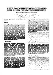
This section presents the details of the experiment, that consists of the process of creating data set in Indonesian emotion speech, speech emotion feature extraction, training, testing , and evaluation. Speech emotion classification is designed in several stages as shown in Figure 1. A. Speech Emotion Data Set The data set of Indonesian speech emotion is created in order to support our research in emotion classification. Speech data set contain short speeches of three semiprofessionals who are trained to imitate speech emotion template. The short speeches include four emotions, such as anger, happiness, sadness and neutral with three different

____________________________________ 978-1-4673-6278-8/13/$31.00 ©2013 IEEE

1015

words. The words are: "diam" (silence), "buka" (open), and "tutup" (close). Each of these words is spoken with intonations that mimicking emotional speech.

windowing process. A window is defined as w(n ) ; then the result of windowing is the signal: ~

x l ( n) = xl ( n) w( n) , where 0 ≤ n ≤ N-1

(3)

The window used in this experiment is Hamming window that has general form: ⎛ 2πn ⎞ w(n) = 0,54 – 0,46 cos ⎜ (4) ⎟ , 0 ≤ n ≤ N-1 ⎝ N −1⎠ 4) Autocorrelation Analysis: Each frame of windowed signal is going through autocorrelation process, then rl (m ) =

N −1− m ~

∑

~

x l ( n) x l ( n + m), m = 0,1,….,p

(5)

n =0

the highest autocorrelation value of p is the order of the LPC. The value of p spreads between 8 to 16. 5) LPC Analysis : The next step is LPC analysis, which changes each frame of p+1 autocorrelations into LPC coefficients. Durbin’s method is used in this analysis. Following equations describe this method:

Figure 1. The design of speech emotion classification

Audio speech signals are recorded by using a good equipment in semi soundproof room. Each utterance is recorded at a sampling frequency of 8 KHz, 16 bit resolution precision, mono channels and in the form of wav files formats. The length of each recording is 1.25 seconds of speech. After the completion of recording process, three participants are asked to do experiment perception test to validate the data set. Almost 40% of the recorded speech do not convince them and discarded. The remaining recorded speech is kept as data set which consist of 360 speech samples.

E(0) = r(0)

⎧

ki = ⎨r (i ) −

⎩

(6) L −1

∑α

( i −1) r j

j =1

⎫

(| i − j |)⎬ ⎭

( i −1)

E

,

where 1 < i < p

α i(i ) = ki α (ji ) = α (ji −1) − kiαi(−i −j j )

B. Speech Emotion Feature Extraction Speech signals are going through feature extraction process using the LPC. The following steps show the basic process of LPC feature extraction [11] : 1) Preemphasis : is used for flattening the spectral purity of the signal and improving the signal on subsequent signal processing. Speech signal s (n ) passes a low order digital system to flatten the spectral signal and remove noise in the signal. The output of Preemphasis ~s (n ) is from the equation: ~ s (n ) = s ( n) − aˆs ( n − 1) where 0.9≤ aˆ ≤1 (1)

E(i) = (1 – ki2 ) E(i-1)

(7) (8) (9) (10)

Equation (6) to (10) are computed with i = 1,2,…,p , and the results are the LPC coefficients or am. The am coefficients themselves are in the forms of : am = αm(p), where 1 ≤ m ≤ p (11) 6) LPC Parameter Conversion to Cepstral Coefficients : The vital set of LPC parameters that are derived directly from the LPC coefficients set is LPC cepstral coefficients, Cm. m −1

Cm

2) Frame Blocking : After the preemphasis step is done, the signal ~ s (n ) is divided into block of frames. Each frame block is comprise of N samples. There are M samples between adjacent frames. Those frames are overlapped, because every next frame is started at M samples after the previous frame. If xl (n) is the lth frame of speech and L frames occurs in the entire speech signal, then: x (n) = ~ (2) s (Ml + n)

k = am + ∑ ⎛⎜ ⎞⎟.Ck .am − k , where 1 ≤ m ≤ p m⎠ k =1 ⎝ m −1 ⎛k⎞ Cm = ∑ ⎜ ⎟.Ck .am − k , where m > p m⎠ k =1 ⎝

(12) (13)

The cepstral coefficients for speech recognition are more reliable than the LPC coefficients [11]. LPC cepstral coefficients are the features extracted from the speech signal. These coefficients are used as input data on machine learning to create a classification model. The speech signals are sampled with sampling frequency at 8 KHz and duration of speech 1.25 seconds. We choose LPC parameter N=240, M=80 and LPC order (p) =10. With these parameters, each speech signal is divided into several

l

where n = 0,1,…,N-1 and l = 0,1,…,L-1 3) Windowing : is done by minimizing the beginning and the end of each signal, hence with both ends become zero, the continuity of the signals is enhanced. After going through the framing process, each frame must go through

1016

frames and frame shifts. Each frame consists of 240 samples. Every frame shift consists of 80 samples. In each speech signal, we have 113 frames. Because each frame has 10 features of LPC cepstral coefficients, thus every speech has 1130 features. The classifiers use these features as input.

algorithm scales indicate someplace between linear and cubic in the train data size. The longest computation time in SMO is in SVM evaluation, thus, for linear SVM, SMO gives the fastest performance. In the actual application of light data sets, SMO is measured to be 1000 times faster than the chunking algorithm [17]. Moreover, there are many kernel options in SMO, one of the kernels is polynomial kernel. Therefore, a polynomial kernel function of SMO is used in this experiment.

C. Speech Emotion Classification Three classifier algorithms are used in this paper, namely Naive Bayes, SMO and MLP, in order to compare the performance of the speech emotion classification: 1) Naive Bayes classifier [15] is a probabilistic classifier based on Bayes theorem that produces probability estimates. The probability of each value that belong to each class is estimated. The advantage of Naive Bayes classifier is that it requires a small amount of training set to estimate the parameters needed for the classification. Naive Bayes assumes that the effect of attribute values in a given class is independent from the value of other attributes. This assumption is called class conditional independent. Naive Bayes classifier estimates the class conditional probability by assuming that attributes are conditionally independent given the class label y. Conditional independent assumption can be expressed in the following form:

(

P XY = y

D. Evaluation Performances of classifier methods are measured using recall, precision and f-measure metrics. The recall is calculated from the amount of speech that is correctly recognized divided by the number of speech that should be recognized. Precision is calculated from the recognized amount of speech that is correctly divided by the total number of recognized speech. F-measure is the harmonic mean of precision and recall. The calculation of recall, precision, and f-measure are stated in (15)-(17) [18] . recall =

) = ∏ P (X i Y = y )

,(15)

# (correctly _ recognized _ recordings)

d

# (correctly_ recognized _ rec.)+ # ( misclassified _ rec.)

(14)

i =1

Each set of attributes X = {X1, X2, ..., Xd} consists of d attributes. 2) MLP classifier is supervised learning algorithm that is used for various applications, such as classification, pattern recognition, prediction and forecasting. Thus, that is the most popular and successful neural network architecture. Moreover, MLP has been used in the domain of speech recognition [16]. An MLP network consists of a number of neurons in each layer. This network has an input layer, hidden layer and output layer. Neural network has only one input and output layer, but the number of hidden layer varies. This paper used one hidden layer with 6 nodes per hidden layer, learning rate equals to 0.3 and momentum equals to 0.2 3) SMO is the most robust training algorithm for support vector machines. The elucidation of huge quadratic programming (QP) optimization problem is required to train a support vector machine. Immense QP problem will be segmented into a sequence of smallest QP problems by using SMO. Moreover, analytical procedure is used to solve the smallest QP problems. This procedure is used to avoid a lengthy numerical QP optimization as an inner loop. Thus, the SMO's memory requirement should be linear in the train data size. As a result, this condition will allow SMO to handle huge train data. However, as the matrix computation is being eluded, the SMO scales indicate someplace between linear and quadratic in the train data size of ranged test problems, and on the other side, standard chunking SVM

precision =

# (correctly _ recognized _ recordings)

,

(16)

# (all _ recognized _ recordings)

f − measure =

2 * recall * precision recall + precision

.

(17)

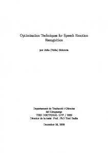
III. EXPERIMENT AND RESULTS This experiment uses 1130 cepstral coefficients features. Performances of three classifier methods (Naive Bayes, SMO and MLP) are compared. The performance measurement is validated using cross validation technique, in order to estimate the accuracy of predictive model performance. One iteration of crossvalidation involved data set separation into two subsets, as to conduct the training set and validate the testing set. We use two types of cross validation technique, the first is 10folds cross validation with a split ratio and the second is Leave-One-Out Cross Validation (LOOCV). The classification results are tested using 10-folds cross validation technique with split ratio as shown in Table I and Figure 2. The percentages of the amount of data used for training and testing varies. Ratio on the training data and testing data start from 10%, with the increase of 10% until it reaches 90%. Each split ratio uses 10-folds cross validation. The 10-folds cross-validation technique divides the data into 10 sub-samples. Testing is repeated 10 times and the measurement result is the average value. The results show

1017

TABLE II.

that best performance of classifier is MLP, with split ratio equals to 80% and accuracy equals to 96.67%.

Emotion Class

TABLE I.

CLASSIFIER PERFORMANCE OF 4 (FOUR) CLASS EMOTION USING 10 FOLDS -CROSS VALIDATION WITH SPLIT RATIO Accuracy (%)

Split Ratio (%)

Naïve Bayes

MLP

SMO

10

48.77

59.14

60.25

20

55.42

71.53

71.74

30

56.98

79.84

82.30

40

54.72

85.56

86.94

50

56.00

91.00

91.33

60

55.97

93.47

94.44

70

52.96

94.07

94.07

80

54.44

96.67

96.39

90

53.33

96.11

95.56

Anger

Neutral

Sadness

Happiness

RESULT OF 4 (FOUR) CLASS EMOTION CLASSIFICATION USING LOOCV Method

Mean Precision (%)

Mean Recall (%)

Mean F-measure (%)

Naïve Bayes

55.60

100.00

71.47

SMO

100.00

97.80

98.89

MLP

97.80

100.00

98.89

Naïve Bayes

37.00

22.20

27.75

SMO

93.60

97.80

95.65

MLP

97.70

95.60

96.64

Naïve Bayes

81.30

28.90

42.64

SMO

95.60

95.60

95.60

MLP

95.60

95.60

95.60

Naïve Bayes

62.50

77.80

69.32

SMO

100.00

97.80

98.89

MLP

100.00

100.00

100.00

In anger emotion class, the result of SMO classifier is equal to 100% for the average of precision. The highest average of recall is 100% as a result from the Naive Bayes and MLP, while the highest average of f-measure is 98.89% as a result from SMO and MLP. For neutral emotional class, the highest average of precision is 97.70% as a result from MLP, the highest average of recall is 97.80% as a result from SMO and the highest average of f-measure is 96.64% as a result from the MLP. For sadness emotion class, the highest average of precision, recall and f-measure are 95.60% as a result from SMO and MLP. In happiness emotions class, SMO and MLP classifiers have 100% as the highest average of precision, while the highest average of recall and f-measure are 100% as a result from MLP. In addition, table II shows that anger emotion class and happiness emotion class more easily classified than neutral emotion class and sad emotion class. This is indicated by the mean of recall, precision and f-measure for anger emotion class and happiness emotion class higher than neutral emotion class and sadness emotion class for all methods of classifier.

Figure 2. Performance of classifier using 10-folds cross validation with split ratio

LOOCV is performed to evaluate the classifiers’ accuracies further. LOOCV involves a single observation from the original sample as the validation data and the remaining observations as the training data. This test is repeated such that each observation in the sample is used once as the validation data. Applying LOOCV is very expensive because the training process is repeated again and again in large number, but LOOCV is able to demonstrate the actual performance of the approach in speech classifiers of real-world applications, since almost all of the training data (except one) must be tested into the classification model. In real implementation, speech classifier uses all training data and should be able to classify a new unknown input [4]. Table II shows the performance of each classifier method for each class of speech emotion.

TABLE III.

CLASSIFIER PERFORMANCE OF 4 (FOUR) CLASS EMOTION USING LOOCV

Method

Mean Recall (%)

Mean Precision (%)

Mean F-measure (%)

Accuracy (%)

Naïve Bayes

57.20

59.10

58.13

57.22

SMO

97.20

97.30

97.25

97.22

MLP

97.80

97.80

97.80

97.78

Table III shows the performance of each classification method that is used to classify the entire classes of speech emotion. MLP generally shows better performance than the other classifiers, in which the accuracy value is 97.78%

1018

compared to 97.22% and 57.22% for SMO and Naive Bayes. For the average of recall and precision shows that the performance of the MLP is also better than other methods.

[6]

[7]

IV. CONCLUSION We have used the classifiers : Naive Bayes, SMO and MLP to classify Indonesian speech emotion data set. LPC method is used to extract speech feature into cepstral coefficients for classification. The experimental results show that MLP has better performance than SMO and Naive Bayes. The average accuracies are equal to 97.78%, 97.22%, and 57.22% respectively. For future work, we will use another feature extraction method of LPC, e.g. Mel Frequency Cepstral Coefficients (MFCC), Zero Crossing Rate (ZCR), and Short Time Energy (STE) for speech emotion classification, and evaluate their performances.

[8]

[9]

[10]

[11] [12]

REFERENCES [1]

[2] [3]

[4]

[5]

[13]

S. A. Firoz, S. A. Raji, and A. P. Babu, “Automatic Emotion Recognition from Speech Using Artificial Neural Networks with Gender-Dependent Databases,” in International Conference on Advances in Computing, Control, Telecommunication Technologies, 2009. ACT ’09, Dec., pp. 162–164. J. Or, Affective Computing, Emotion Expression, Synthesis and Recognition. I-Tech Education and Publishing, 2008. S. Yun and C. D. Yoo, “Loss-Scaled Large-Margin Gaussian Mixture Models for Speech Emotion Classification,” IEEE Transactions on Audio, Speech, and Language Processing, vol. 20, no. 2, pp. 585– 598, Feb. 2012. S. Sumpeno, M. Hariadi, and M. H. Purnomo, “Facial Emotional Expressions of Life-like Character Based on Text Classifier and Fuzzy Logic,” IAENG International Journal of Computer Science, 38:2, pp. 122–133, 2011. C. Busso, S. Lee, and S. Narayanan, “Analysis of Emotionally Salient Aspects of Fundamental Frequency for Emotion Detection,” IEEE Transactions on Audio, Speech, and Language Processing, vol. 17, no. 4, pp. 582–596, May 2009.

[14]

[15] [16]

[17]

[18]

1019

Y. Shi and W. Song, “Speech emotion recognition based on data mining technology,” in 2010 Sixth International Conference on Natural Computation (ICNC), Aug., vol. 2, pp. 615–619. T. Iliou and C.-N. Anagnostopoulos, “SVM-MLP-PNN Classifiers on Speech Emotion Recognition Field - A Comparative Study,” in 2010 Fifth International Conference on Digital Telecommunications (ICDT), June, pp. 1–6. I. Luengo, E. Navas, and I. Hernáez, “Feature Analysis and Evaluation for Automatic Emotion Identification in Speech,” IEEE Transactions on Multimedia, vol. 12, no. 6, pp. 490–501, Oct. 2010. A. A. Razak, R. Komiya, M. Izani, and Z. Abidin, “Comparison between fuzzy and NN method for speech emotion recognition,” in Third International Conference on Information Technology and Applications, 2005. ICITA 2005, 2005, vol. 1, pp. 297–302 vol.1. I. R. Murray and J. L. Arnott, “Toward the simulation of emotion in synthetic speech: a review of the literature on human vocal emotion,” J. Acoust. Soc. Am., vol. 93, no. 2, pp. 1097–1108, Feb. 1993. L. R. Rabiner and B. B.-H. Juang, Fundamentals of Speech Recognition. Prentice Hall, 1993. J. Cho and S. Kato, “Detecting emotion from voice using selective Bayesian pairwise classifiers,” in 2011 IEEE Symposium on Computers Informatics (ISCI), 2011, pp. 90–95. S. Casale, A. Russo, G. Scebba, and S. Serrano, “Speech Emotion Classification Using Machine Learning Algorithms,” in 2008 IEEE International Conference on Semantic Computing, 2008, pp. 158– 165. J. Wang, Z. Han, and S. Lung, “Speech emotion recognition system based on genetic algorithm and neural network,” in 2011 International Conference on Image Analysis and Signal Processing (IASP), Oct., pp. 578–582. J. Han, M. Kamber, and J. Pei, Data Mining: Concepts and Techniques, Third Edition, 3rd ed. Morgan Kaufmann, 2011. A. Ahad, A. Fayyaz, and T. Mehmood, “Speech recognition using multilayer perceptron,” in IEEE Students Conference, 2002. ISCON ’02. Proceedings, 2002, vol. 1, pp. 103–109 vol.1. J. C. Platt, “Sequential Minimal Optimization: A Fast Algorithm for Training Support Vector Machines,” Microsoft Research Technical Report MSR-TR-98-14, Apr. 1998. S. Ntalampiras and N. Fakotakis, “Modeling the Temporal Evolution of Acoustic Parameters for Speech Emotion Recognition,” IEEE Transactions on Affective Computing, vol. 3, no. 1, pp. 116–125, 2012.