JUNE 2001
TIMMERMANN ET AL.
1579
Empirical Dynamical System Modeling of ENSO Using Nonlinear Inverse Techniques A. TIMMERMANN KNMI, De Bilt, Netherlands
H. U. VOSS Physics Department, University of Freiburg, Freiburg, Germany
R. PASMANTER KNMI, De Bilt, Netherlands (Manuscript received 29 September 1999, in final form 8 September 2000) ABSTRACT A statistical technique is presented that allows for the empirical derivation of dynamical system equations from data. It is based on multiple nonparametric regression analysis and is applicable to a broad class of physical systems. It is applied to differential delay equations as well as to ordinary differential equations. The aim of this paper is to illustrate this technique in the context of the El Nin˜o–Southern Oscillation (ENSO) phenomenon. A set of reduced models is derived from an intermediate coupled atmosphere–ocean model of the tropical Pacific and from a state-of-the-art coupled general circulation model simulation. The analysis in this paper focuses on the dimensionality issue as well as on the role of nonlinearities. The empirical technique presented in this study helps to identify key ENSO processes and to explain physical peculiarities of ENSO simulations.
1. Introduction The El Nin˜o–Southern Oscillation (ENSO) phenomenon, the strongest natural interannual climate fluctuation, originates in the tropical Pacific but affects climate conditions globally. ENSO is an irregular low-frequency oscillation between a warm (El Nin˜o) and a cold state (La Nin˜a) with a preferred timescale of 2–8 years. ENSO extremes have a strong impact on the societies of many countries as well as on sensitive ecological systems. Among other effects, typical El Nin˜o events are associated with poor monsoon rains in India, droughts in Indonesia, Australia, the Northeast of Brazil, and southern Africa, and flooding in coastal Peru and Ecuador, the southern cone of South America, and the Great Basin of the United States. El Nin˜o events have been shown to be responsible for high incidences of malaria in the Punjab, poor maize harvests in Zimbabwe and reduced wheat crops in Australia. It is estimated that the 1982/ 83 El Nin˜o caused U.S. $13 billion in damage worldwide and was responsible for about 2000 deaths. The impacts of the even stronger 1997/98 El Nin˜o were somewhat mitigated by prediction and monitoring based Corresponding author address: Dr. Axel Timmermann, IPRC, SOEST, University of Hawaii at Manoa, 2525 Correa Road, Honolulu, HI 96822. E-mail:
[email protected]
q 2001 American Meteorological Society
on the marked increase in our understanding in the intervening 15 years. Hence, prediction of ENSO-related climate anomalies and their societal and ecological impacts has become an important part of climate research. Our understanding of ENSO rests on a hypothesis first put forward by Bjerknes (1969), and supplemented by a later understanding of equatorial ocean dynamics (Neelin et al. 1998). Positive temperature anomalies in the eastern equatorial Pacific (characteristic of an El Nin˜o event) reduce the sea surface temperature difference across the tropical Pacific. Consequently, the trade winds weaken and the Southern Oscillation index (defined as the sea level pressure difference between Tahiti and Darwin) becomes negative. At the same time, these weakened trades reduce the upwelling of cold water in the eastern equatorial Pacific, thereby strengthening the initial positive temperature anomaly. However, they also trigger negative off-equatorial thermocline depth anomalies in the central and western Pacific. These anomalies propagate westward to the coast, where they are reflected to propagate eastward along the equator. Thus, at some delay from when they were generated these negative anomalies cause the temperature anomaly in the east to decrease and change sign. The combination of the tropical air–sea instability and the delayed negative feedback due to subsurface ocean dynamics can give rise to oscillations (Schopf and Suarez 1990; Suarez and
1580
JOURNAL OF PHYSICAL OCEANOGRAPHY
Schopf 1988; Battisti and Hirst 1989; Cane et al. 1990; Mu¨nnich et al. 1991; Tziperman et al. 1994, 1998; Jin 1997). Large-scale temperature anomalies during an El Nin˜o event heat the atmosphere very effectively, which leads to changes of the global atmospheric circulation. The ENSO phenomenon is investigated using a whole hierarchy of models: R R R R R
conceptual models statistical models intermediate coupled models hybrid coupled models coupled general circulation models.
Conceptual models for ENSO are the simplest models in a hierarchy of models of different complexity. They are designed to capture some of the crucial characteristics of ENSO in an intuitively understandable manner. These models have a big impact on our understanding of ENSO. The most prominent candidates are the delayed action oscillator model (Schopf and Suarez 1990; Suarez and Schopf 1988; Battisti and Hirst 1989; Cane et al. 1990) and the ocean recharge oscillator model (Cane et al. 1990; Jin 1997; Wyrtki 1986). The delayed action oscillator concept, which will be treated in our study as a zero-order ENSO model, was first derived by Battisti and Hirst (1989), Suarez and Schopf (1988), and Schopf and Suarez (1990) from the reduced-gravity shallow-water equations on an equatorial beta plane. The atmosphere–ocean instability can be crudely parameterized in terms of a linear relationship and a cubic damping term. Assuming localized atmosphere–ocean coupling and short Kelvin wave delay times, Schopf and Suarez (1990) and Battisti and Hirst (1989) obtained the following prognostic nondimensional temperature equation: dT(t) 5 T(t) 2 aT(t 2 t ) 2 T 3 (t). dt
(1)
For vanishing Rossby wave delay time t this differential delay equation reduces to an ordinary differential equation, which undergoes a pitchfork bifurcation at a 5 1. On the other hand, if the time derivative can be neglected, Eq. (1) has some characteristics of a map. Equation (1) is at the core of our intuitive understanding of ENSO. It explains why the dominant period of ENSO is longer than the sum of the delay times. However, it explains neither the phase locking of ENSO to the annual cycle nor the observed irregularity. Statistical/empirical models are based on the assumption that ENSO can be parameterized in terms of stochastic dynamics. The hierarchy of statistical models ranges from simple univariate autoregressive moving average-type models (Trenberth and Hoar 1996; Burgers 1999; Zwiers and von Storch 1990) to multivariate linear models (e.g., Penland 1989; Blumenthal 1991) based on the principle oscillation pattern (POP) ansatz (Hasselmann 1988) or Canonical Correlation Analysis (Preisendorfer 1988). These statistical models are success-
VOLUME 31
fully applied in the ENSO prediction context (Penland and Magorian 1993; Xue et al. 1994; Johnson et al. 2000) or in order to assess the unusualness of particular ENSO situations (Trenberth and Hoar 1996). Statistical ENSO models have so far focused only on linear dynamics, while attributing ENSO irregularity to the driving noise source. The approach pursued here is to our knowledge one of very few nonlinear empirical approaches (Grieger and Latif 1994) in ENSO modeling. In fact, we do believe that part of the unresolved noise in linear models can be disentangled in terms of deterministic nonlinear dynamics. Whether this also has significant impact on ENSO predictability will be addressed in a forthcoming study. Intermediate coupled models: Physical ENSO modeling started with coupled atmosphere–ocean models of intermediate complexity. These coupled models capture the crucial physical processes in a compressed form. The most famous intermediate coupled model is the Zebiak and Cane model (Zebiak and Cane 1987), which consists of a shallow-water ocean model on an equatorial beta plane and a steady-state response tropical atmosphere. The main characteristic of these models is that they employ effective approximations to the true equations. Their simplicity allows one to explore the phase and parameter space in a systematic way. Furthermore, they have also been quite successful in the ENSO prediction context. Approximate analytical solutions can be derived (Cane et al. 1990; Jin 1997; Mu¨nnich et al. 1991) that have helped in formulating ENSO paradigms such as the delayed action oscillator and the ocean-recharge paradigm. Hybrid coupled models consist of a statistical model for the atmospheric anomalies and an ocean model based on the primitive equations. The crucial simplification rests on the observation that atmospheric anomalies in the Tropics can be diagnosed to a very large extent from the tropical SST anomaly field. A very elegant formulation of the statistical atmospheric model was suggested in Barnett et al. (1993). This formulation exploits the covariant structure of tropical wind stress and SST anomalies in EOF space. Such hybrid coupled models are used also in the ENSO prediction context (Barnett et al. 1993; Flu¨gel and Chang 1996; Blanke et al. 1997; Eckert and Latif 1997). Coupled general circulation models (CGCMs) stand at the top of the hierarchy. They consist of an ocean– atmosphere general circulation model and a sea ice model. The dynamical equations to be solved for the atmosphere and the ocean are the primitive equations for each medium, respectively. This set of equations is a filtered version of the Navier Stokes equations on a sphere. Unresolved and diabatic processes are parameterized. The complexity of these models forbids a detailed exploration of the phase and parameter space. It is the goal of many climate research centers to develop CGCMs and to apply them under different climate conditions. This helps in predicting the climate of the twen-
JUNE 2001
1581
TIMMERMANN ET AL.
ty-first century and to reconstruct past climates. However, CGCMs are only of limited use in generating new ideas and metaphors on the climate system. ‘‘Understanding’’ is also a process of simplification and abstraction. Thus, the development of CGCMs has to go hand in hand with strategies to simplify complexity and to formulate reduced models for particular climate phenomena. The goal of this paper is to derive empirically a whole hierarchy of empirical dynamical models (in terms of univariate differential delay equations and multidimensional ordinary differential equations) for ENSO that optimally reproduce the dynamics of the data under consideration. We will use ENSO data obtained from an intermediate coupled atmosphere–ocean model as well as from a CGCM simulation. Hence, our approach connects the statistical model approach discussed above with the others. In section 2 the mathematical strategy will be outlined. We sketch a methodology that is able to derive the Frobenius Perron operator of a nonlinear dynamical system statistically. Section 3 illustrates how this method is applied to derive differential delay equations from data simulated by given dynamical equations. In section 4 the maximal correlation method is applied to estimate optimal differential delay equations from an ENSO simulation performed with an intermediate coupled atmosphere–ocean model. The same simulation is used in order to reconstruct a whole hierarchy of ordinary differential equation models. Our analysis focuses on the role of nonlinearities and tries to isolate key processes relevant for ENSO. A similar analysis is presented in section 5, which focuses on the statistical derivation of optimal dynamical equations from ENSO data obtained from a coupled general circulation model. We discuss how the space–time structure of ENSO changes with changing number of degrees of freedom. Furthermore, we explore the role of higher order nonlinearities. Our paper concludes with a summary and a discussion of our results, in section 6.
where p( · | · ) denotes the conditional probability density function. Due to the relation p(x˙ j | x) 5 p(x˙ j , x)/p(x) the estimation of the optimal transformation becomes equivalent to the estimation of a multidimensional probability density function. Even for small system dimensionality N this is often practically impossible. In climate dynamics observational datasets are too short and too noisy to apply this strategy successfully. We propose the following alternative: For many problems it is not necessary to solve the general reconstruction problem. On the basis of some a priori knowledge of the probability density function the reconstruction problem simplifies considerably. We assume that the model equation (2) can be approximated by a combination of general transformations F ij(x i ); that is, x˙ j 5
O F (x ) 1 s j , j i
i
(4)
j
j
i51
where the mismatch between (2) and (4) is parameterized in terms of white noise ^j j(t)j k(t9)& 5 d jk d(t 2 t9) of variance s j 2 . Equation (4) defines a nonlinear multiple regression problem. It is solved with the ACE (Alternating Conditional Expectation Value) algorithm of Breiman and Friedman (1985). The ACE algorithm converges in a consistent way to optimal transformations defined by Eq. (4), as has been shown also in Breiman and Friedman (1985). Here we use a modified algorithm, where the modification consists of fixing the lhs of Eq. (4), whereas in Breiman and Friedman (1985) it is also varied. For details on the numerical implementation of the ACE algorithm see Voss (2000), Voss and Kurths (1997), and Voss et al. (1999). (A MATLAB-program and a C-program can be obtained from the authors or from the Web page at http://www.fdm.uni-freiburg.de/ ; hv/hv.html.) The modified ACE algorithm works as follows: Globally optimal solutions [in a least squares ˜ ij (x i )) 2 & 5 min] can be obtained sense, i.e., ^(x˙ j 2 S i51 F iteratively from the sequence ˜ i,j 0 (x i ) 5 ^x˙ j | x i &, F
2. Strategy In the context of dynamical system modeling one very often encounters the problem to determine the relation F that maps x˙ jt 5 F j(x t),
(2)
where x t 5 (x1t , · · · , x ti , · · · , x tN )T is the N-dimensional data vector at time t, and x˙ jt represents the time derivative of the jth component at time t. In the following we omit the time index t. In order to find the transformation F˜ that solves Eq. (1) in a least squares sense, the expectation value of x˙ j conditioned on x has to be determined. In general, the optimal transformation can be estimated as the conditional expectation value F˜ j (x) 5
E
p(x˙ j | x)x˙ j dx˙ j ,
(3)
7 O
˜ i,j k (x i ) 5 x˙ j 2 F
p±i
(5)
)8
˜ p,j k* (x p ) x i . F
(6)
The index j corresponds to the component of the differential equation, k to the iteration step (k . 0), and p to the sum over the predictor components. The index k* equals k for p , i and k 2 1 for p . i, ^ · · | · · & denotes the conditional expectation value. The so-called j ˜ i,k optimal transformations F (x i ) produced by this algorithm are given in the form of numerical tables. In the expression (6) only scalar quantities are involved and, in contrast to Eq. (3), only one-dimensional conditional probabilities (or, equivalently, two-dimensional joint probabilities) have to be estimated. These can be interpreted in terms of the time transition probabilities or as the dynamical contribution to the component-wise
1582
JOURNAL OF PHYSICAL OCEANOGRAPHY
Frobenius Perron operator of the underlying dynamical system. Minimizing ^(x˙ j 2 S i51 F ij (x i )) 2 & is equivalent to the maximization of the correlation
O F˜ (x )8 7 C(x˙ , x , · · · , x ) 5 5^x˙ &7[O F˜ (x )] 86 N
x˙ j
j i
i
i
j
1
N
2
N
j2
j i
1/ 2
,
(7)
where it is assumed that all variables have zero mean. Hence, this technique to solve the nonlinear regression problem is also called maximal correlation approach. Deriving nonlinear models empirically can be highly nontrivial if it is intended not only to fit the dynamics but to identify the fitted components with physical processes and sensitivities. Our goal here is to derive empirically global1 equations of motion for the dynamical system under consideration and to build up an understanding of the underlying physics. If such equations of motion are derived only for prediction purposes, the scientific requirements are much lower than in our case. In the prediction context only tendency errors of the variables x i have to be minimized. No physical interpretation of the components is required. In our situation one is faced with the problem of selecting the ‘‘correct’’ functional forms for the global model out of an infinite set of functions. The combination of nonparametric regression analysis and the maximal correlation method provides some objective means for extracting the optimal functionals. Furthermore, we impose restrictions to the optimal model by choosing an ansatz for the equations of motion that is physically meaningful. In the context of empirical dynamical system modeling a more general problem emerges: The dynamical equations will be derived from just one system trajectory. Therefore, we cannot expect an overall validity throughout the whole system state space. As discussed in Abarbanel (1997), a different set of initial conditions might lead to a different behavior of the system. In this new basin of attraction it is unlikely that our empirical model operates in the same manner as it does in the original part of the system state space. This criticism against models that use empirically derived corrections or parameterizations is quite general. In principle CGCMs also contain a huge amount of parameterizations that had been calibrated on present day observations. There is no a priori certainty that these empirically derived functional forms remain the same when considering past or future climates. 3. Estimation of nonlinear dynamical systems by the maximal correlation method For the purpose of illustration the maximal correlation method sketched above will be applied to the Tziperman 1
In the sense of dynamical system analysis.
et al. (1994) delayed action oscillator (DAO) model, which can be regarded as a paradigmatic ENSO model. Our goal is to recover the DAO model equation for the thermocline depth anomalies x˙ 5 af [x(t 2 t 1 )] 1 bf [x(t 2 t 2 )] 1 c cos(2pn0 t) (8) with f (x) 5 b tanh(kx/b),
i
i
VOLUME 31
b5
5
1.5, 0.3,
x$0 otherwise
(9)
from a simulated time series. The nonlinear function f relates wind stress anomalies to thermocline anomalies, thereby representing the atmosphere–ocean sensitivity. The first delay term is associated with the positive Kelvin wave feedback, whereas the second delay term relates to the negative Rossby wave feedback. As pointed out by Mu¨nnich et al. (1991), f can be regarded as a crude representation of the temperature shape in the thermocline region. In that perspective k determines the thermocline slope and a and b quantify the amplitude of the atmosphere–ocean coupling. The annual cycle strength is denoted by c and the annual cycle frequency by n 0 (fn2). A comparison between Eqs. (4) and (8) shows that by setting s j 5 0, x1 5 x1 , x 2 5 x1(t 2 t1), and x 3 5 x1(t 2 t 2) the reconstruction problem can be solved using the maximum correlation for j 5 1. To estimate the optimal delay times t1 , t 2 , the ACE algorithm is applied for each possible t1 , t 2 pair. The values of t1 , t 2 that maximize C(x˙1 , x1(t 2 t1), x1(t 2 t 2)) represent the optimal choice for the delay model. This method has been successfully applied both to several simulated datasets (Voss and Kurths 1997) and to experimental measurements (of a laser ring resonator experiment) (Voss et al. 1999). The maximal correlation method is applied here by using a simulated time series of thermocline depth anomalies with 500 data points, corresponding to 500 weeks (Fig. 1a). For the numerical integration of Eq. (8) a fourth-order Runge Kutta scheme is used, with the ‘‘standard’’ parameters a 5 1/180, b 5 21/120, c 5 1/138, k 5 2, n 0 5 1/60 (Fn3), t1 5 5.83 weeks, and t 2 5 29.17 weeks, such as to account for quasiperiodicity and potential chaos. Applied to the ansatz (8), the maximal correlation method yields a maximal correlation of 0.9958 for the delay pair (t1 , t 2 ) 5 (6, 29), as shown in Fig. 2a. Furthermore, it can be seen that the fit of a one-delay model (Fig. 2b) yields smaller values for the maximal correlation (0.968) than using the two-delay ansatz. This is 2 Whether it is suitable to include the annual cycle additively rather than in a multiplicative form (see Mu¨nnich et al. 1991) shall not be discussed here. 3 One year is assumed here to have 60 weeks.
JUNE 2001
TIMMERMANN ET AL.
1583
FIG. 1. (a) Simulated time series of the Tziperman model [Eq. (8)]; (b), (c) estimated (dotted) delayed feedback terms; and (d) estimated annual cycle. In (b)–(d), the model functions of Eq. (8) are represented by solid lines. The time unit is one week.
another indication for the inherent two-delay dynamics in the time series. Figures 1b–d display the estimated optimal transformations representing the delayed feedback terms and the cyclostationary forcing. One observes a very good agreement between estimated and theoretical curves. The deviations are due to the shortness of our dataset.
As a further result, the seasonal forcing term has been estimated with high accuracy. In the case of short time series, sample fluctuations can induce artificial dependencies, even in statistically independent data, which are also recovered by the maximal correlation. Therefore, the numerical estimate of the maximal correlation from finite datasets deviates
FIG. 2. (a) Maximal correlation C(t1 , t 2 ) obtained from the simulated thermocline depth anomalies in Fig. 1 using a two-delay model. Dark areas indicate small values, white areas large values. The maxima at ( t1 , t 2 ) 5 (6, 29) and (29, 6) are marked with 1 symbols. The time unit is one week. (b) Maximal correlation C(t) using a one-delay model. Maxima are located at t 5 4 and t 5 33.
1584
JOURNAL OF PHYSICAL OCEANOGRAPHY
TABLE 1. Five percentile quantiles q 5 of the asymptotic distribution of the estimate for C, assuming no statistical dependence (i.e., C 5 0), for N 5 100, · · · , 1000 data points. N
q5
100 200 300 500 1000
0.623 0.441 0.359 0.278 0.197
from its asymptotic value for infinitely large datasets. In particular, it is biased towards too large values (Sethuraman 1990). In order to document the statistical significance of the null hypothesis ‘‘C ± 0,’’ Table 1 shows the 5% quantiles of the maximal correlation as a function of the number of data points. In this example and in all following calculations, the estimates for delay times always correspond to a maximal correlation that is well above these 5% quantiles. The example given above confirms the results of Voss and Kurths (1997), Voss et al. (1999), and Voss (2000): the ACE algorithm is a very powerful method of estimating delayed feedback dynamics from short datasets. This success motivates our next step. 4. Reducing ENSO dynamics of an intermediate model In this section the method sketched above will be applied to the Zebiak and Cane (ZC) ENSO simulation model (Zebiak and Cane 1987). The ZC model is a coupled atmosphere–ocean model for the tropical region. The atmospheric component consists of a Gilltype steady-state linear shallow-water model (Gill 1980) formulated on an equatorial beta plane. Dissipation is parameterized in terms of linear Newtonian cooling and Rayleigh friction. Furthermore, a surface-wind parameterization of low-level moisture convergence is used. This model simulates the steady-state atmospheric response to typical sea surface temperature anomalies (SSTAs) in the Tropics reasonably well. The ocean model is formulated for a rectangular tropical ocean basin. It is based on a linear reduced-gravity model, including a shallow frictional layer of 50 m depth, which accounts for surface intensification of wind-driven currents. The thermodynamic core of this ocean model takes into account three-dimensional temperature advection by mean and anomalous ocean currents, a linear dependence between surface heat flux anomalies and SSTA and the asymmetric effect of vertical advection on temperature. Subsurface temperature anomalies are diagnosed from the variations of the model’s upper-layer thickness. The seasonal background fields of surface winds and wind divergence, as well as of sea surface temperature, are prescribed. First we reduce the simulated ENSO dynamics of the ZC model to an optimal differential delay equation. The
VOLUME 31
maximal correlation method sketched and illustrated above is applied to the simulated 10-daily sampled Nin˜o-3 SSTA time series (37 years of SSTA averaged over the region 58S–58N, 1508W–908W), abbreviated by x(t). Despite the rather unrealistic representation of the annual cycle in model equation (8) we fit a similar delay model to the SSTA time series data under consideration. It has the form x˙ 5 F1 [x(t 2 t 1 )] 1 F2 [x(t 2 t 2 )] 1 G(t, mod 36).
(10)
Browsing through all possible delays with t1 , t 2 , 300 days we find that the maximal correlation of approximately 0.8 is attained for t1 5 40 and t 2 5 250 days, corresponding to the expected Kelvin wave delay and the first Rossby mode delay time, respectively.4 The corresponding optimal transformations are depicted in Fig. 3. Although the estimated optimal delay pair is very close to the values of the heuristic delayed action oscillator model of Tziperman et al. (1994), the optimal transformations differ quite a bit. Here F1 describes a positive feedback for positive SST anomalies. However, large negative SST anomalies are associated by the optimal transformations with a positive temperature tendency, which seems unphysical. The variance of F1 quantifies roughly the relative magnitude of the Kelvin wave effect as compared to the negative Rossby wave feedback, represented by F 2 in Fig. 3. This wave interpretation is motivated by the findings of Mu¨nnich et al. (1991), who derived analytically differential delay equations from a physical model. It should be noted here that the optimal transformations represent only a first-order approximation to the dynamical system. They are uncertain due to the length of the original timeseries, unresolved dynamics not captured by the model ansatz, and initial value problems. These uncertainties are typical for empirical modeling and difficult to assess systematically. Even in linear stochastic modeling the uncertainity in estimating empirical model parameters is often not taken into account (Trenberth and Hoar 1996). In order to perform forward and sensitivity integrations with the reconstructed delay model we fit the optimal transformation F1 , F 2 , and G by a sixth-order polynomial.5 The result of the forward integration of this parameterized model is shown in Fig. 4. One observes that the delay model captures both the dominant period as well as the mean amplitude of the original Nin˜o-3 SSTA very well. The quality of the empirical model simulation can be furthermore quantified by using higher-order statistical moments. As can 4 One could also account for the annual cycle forcing in terms of multiplicative terms. Different representations of the annual cycle forcing might further increase the maximal correlation. This issue will be addressed in a forthcoming study. 5 The aforementioned uncertainty in estimating the parameters of the analytical model is not taken into account here.
JUNE 2001
TIMMERMANN ET AL.
1585
FIG. 3. (top left) F1 1 F 2 1 G vs the estimated time derivative (linear regression fit indicated by thick points). A straight line with slope 1 indicates a high correlation. Optimal transformations F1 [x(t 2 t1 )], F 2 [x(t 2 t 2 )] and G(t, mod 360 days) and fitted sixth-order polynomials, rhs of Eq. (10). A 37-yr-long 10-daily sampled Nin˜o3 SSTA index was used for the reconstruction.
be seen from Fig. 4 the fact that in the original time series large positive anomalies are more likely than negative anomalies (as characterized by the skewness of the distribution) is captured by the empirical model. The exact value of the skewness, however, is not reproduced sufficiently well. The skewness of the probability distribution is a manifestation of nonlinear processes acting in the system. It is unlikely that a single delay equation can capture all of the dynamics and nonlinearities of the ZC model.6 The estimated dynamical models (using third-, fifth-, and sixth-order polynomial fits for F1 , F 2 , G) can be used in order to assess how sensitive ENSO is with
FIG. 4. Nin˜o SST anomalies simulated by the ZC model (dashed curve) Nin˜o-3 SST anomalies simulated by the optimal differential delay equation obtained from dashed curve (solid thick curve).
6 An objective way to quantify the similarity between original time series and simulated time series would be to address the following questions: Are the spectra of the time series seen as statistically equal? Do the probability distributions differ? The former question can be answered by using chi-squared statistics, whereas the latter can be tackled by standard nonparametric tests such as the Mann–Whitney U test. We do not apply these tests here since it is not the aim to reproduce the full dynamics but to capture and simulate the essential dynamical features.
1586
JOURNAL OF PHYSICAL OCEANOGRAPHY
VOLUME 31
FIG. 5. Stroboscopically sampled (10-yr sampling frequency) Nin˜o-3 SST anomalies for different amplitudes a of the negative feedback component simulated by a third, fifth, and sixth order polynomial differential delay equation.
respect to changes of the system, such as increased amplitude of the annual cycle, stronger negative and positive feedback terms, etc., and the degree of nonlinearity. Figure 5 shows the bifurcation diagram of SST anomalies simulated by a third-, a fifth-, and a sixth-order polynomial model. The diagram is obtained by stroboscopically sampling the simulated SST anomalies with a 10-yr period for different negative feedback term amplitudes a. The analytical equation fitted to the optimal transformations in Fig. 3 has the form
O p x (t 2 t ) 1 a O q x (t 2 t ) 1 O r (t, mod 360 days), N
x˙ 5
N
i
i
i
1
i50
i
2
i50
6
i
(11)
i51
with N either 3, 5, or 6. One observes that for small amplitude a, that is, when the effect of the Rossby waves to the temperature equation is small, the simulated temperature anomalies vanish. The temperature evolution is characterized by an annual cycle. In phys-
ical terms this indicates that the delayed negative feedback due to Rossby waves is crucial for the generation of interannual ENSO variability (see also Battisti and Hirst 1989). This type of variability emerges from a Hopf bifurcation for values of a of around 0.9–1.1, depending on the degree of nonlinearity. One observes for all three polynomial models transitions from periodic to quasiperiodic behavior and also chaotic regime transitions. The degree of the highest polynomial in the analytical delay model determines the exact location and also the appearance of transitions and bifurcations. However, some overall features are robust: the emergence of a Hopf bifurcation and an increase of the amplitude of SST anomalies as the Rossby wave amplitudes increase. Due to the rather crude representation of the annual cycle in our model we skip the sensitivity analysis of ENSO with respect to the annual cycle. We next apply the ACE algorithm to a system of ordinary differential equations (ODEs) to be derived from the SSTA and thermocline depth anomaly data simulated by the ZC model.
JUNE 2001
1587
TIMMERMANN ET AL.
FIG. 6. Dominant EOF patterns of sea surface temperature anomalies (top) and thermocline depth anomalies (bottom). Patterns are dimensionless.
In order to simplify the system in a physically meaningful sense, we reduce the number of degrees of freedom of the simulated temperature and thermocline fields by performing an empirical orthogonal function (EOF) analysis on the 37-year-long dataset. Only the two leading EOFs of both temperature and thermocline depth anomalies are retained (shown in Fig. 6) because they can be interpreted in terms of physical features. These EOFs account cumulatively for about 90% and 80% of the temperature and thermocline depth data variance, respectively. The first EOF pattern for SSTA represents the mature ENSO signal, whereas the second pattern can be interpreted as a precursor to the mature phase, due to Kelvin wave propagation. The first thermocline mode clearly represents the Rossby wave precursor to an El Nin˜o or a La Nin˜a event. The second thermocline depth mode corresponds to different thermocline adjustment contributions. From the corresponding principal components shown in Fig. 7 (x1 5 T1 , x 2 5 T 2 for temperature anomalies and x 3 5 H1 , x 4 5 H 2 for thermocline depth anomalies)
a set of ordinary differential equations is constructed based on the following ansatz:
O F (x ), A
x˙ k 5
k i
i
(12)
i51
where the indices k, 5 1, · · · , 4 and A # 4. The optimal ˜ ki are obtained by means of nonlinear transformations F multiple regression analysis combined with the maximal correlation method.7 a. 2-EOF model In order to facilitate the physical interpretation we first focus on a class of models, with A 5 2, that is, we take into account only the first temperature and the first 7 In this analysis we do not take into account the seasonality because, using the ACE algorithm in its present form, it is difficult to implement it such that, for example, multiplicative effects (like cos(vt)F i (xi)) could be taken into account.
1588
JOURNAL OF PHYSICAL OCEANOGRAPHY
VOLUME 31
FIG. 7. Leading principal components for temperature anomalies (T1 , T 2 ) and thermocline depth anomalies (H1 , H 2 ) simulated by the ZC model. The standard deviation of the time series are indicated on top of each figure.
thermocline depth anomaly EOF. We apply the ACE algorithm to the computed time derivatives (accuracy of fourth order in the time step is taken into account) x˙1 and x˙ 3 and the arguments x1 , x 3 . The maximal correlations attain values of about 0.85. The optimal transformations are approximated by polynomials of different order P, and the resulting set of equations ˙x˜k 5 S i51,3 S Pj51 r ji, k x˜ ij (k 5 1, 3) is integrated forward in time for 37 years by means of the fourth-order Runge Kutta scheme. The result for P 5 1, that is, a linear interpolation, gives rise to an unstable oscillation (not shown here). However, the ZC model simulates a bounded ENSO, which implies that either higher-order nonlinearities P . 1 or neglected higher-order EOFs have a damping effect on the linearized ENSO dynamics. We have found (simulated principal components not displayed here) that a cubic interpolation to the optimal transformations yields a stable ENSO cycle with a period of 4 years, which is very close to the original period of 3.7 years. The boundedness of the solution obtained with the cubic 2-EOF model illustrates the fact that nonlinearities have a crucial effect on ENSO dynamics within the context of the ZC model. They stabilize the linearly unstable 2-EOF model. It turns out that cubic
polynomials are enough in order to approximate the numerically given optimal transformations. Despite the fact that the nonlinear 2-EOF model generates interannual oscillations it is not a realistic model from the physical point of view. In order to visualize the reconstructed evolution of ENSO for the 2-EOF model, including cubic nonlinearities, we show in Fig. 8 a set of SSTA and thermocline depth Hovmo¨ller diagrams along the equator and at 148S. The reconstructed SSTA vector is obtained from T(t) 5 x˜1(t)e T,1 and the reconstructed thermocline depth vector from D(t) 5 x˜ 3(t)e D,1 . The first EOF patterns for temperature and thermocline depth anomalies are denoted by e T,1 and e D,1 , respectively. One observes standing SSTA and thermocline depth oscillations and a characteristic phase relationship between surface quantities in the eastern equatorial Pacific and subsurface quantities in the western equatorial Pacific. The next step in our analysis is to take into account more degrees of freedom. b. 4-EOF model In order to allow for spatial propagation of thermocline depth anomalies in time one has to take into ac-
JUNE 2001
TIMMERMANN ET AL.
1589
FIG. 8. Hovmo¨ller plot of temperature (Trecon ) (K) and thermocline depth (Hrecon ) anomalies (m) along the equator (upper panels) and at 148S (lower panels). The anomalies are simulated on the basis of the 2-EOF model and cubic interpolation of the optimal transformations.
count higher-order EOF modes. Therefore, a 4-EOF model will be estimated from the two leading temperature and two leading thermocline depth principal components. The resulting optimal transformations are fitted using a cubic interpolation for the reasons given in the previous paragraph. Eventually the approximated set of ordinary differential equations is integrated forward in time. The maximal correlations between the tendencies and the optimal transformations of the different principal components attain values of about 0.85–0.97. The resulting ‘‘reconstructed’’ principal components (not shown) are multiplied back onto the EOF patterns in order to reconstruct the SSTA and thermocline depth anomaly fields. We compute a Hovmo¨ller diagram of these fields along the equator and at 148S. The Hovmo¨ller diagram (shown in Fig. 9) is characterized by eastward propagating thermocline depth anomalies on the equator and westward propagating subsurface anomalies off the equator. Furthermore, as can be seen from Fig. 9, the ENSO phase transition (from warm to cold and vice versa) is characterized by a zonal near-uniform thermocline depth anomaly being reminiscent of the ocean recharge par-
adigm (Jin 1997). The 4-EOF model8 can thus be interpreted in terms of the ocean recharge oscillator (Jin 1997). Obviously the inclusion of second-order EOF modes changes the dynamical behavior and in particular the period and irregularity of ENSO considerably. 5. Reducing ENSO dynamics of a coupled general circulation model To study whether the strategy to derive reduced models carries over to more complex and noisy systems we analyze the ENSO simulated by a control (present day atmospheric greenhouse concentrations) experiment. This experiment was conducted with the coupled general circulation model ECHAM4/OPYC3. The atmosphere model ECHAM4 is coupled to the isopycnal ocean model OPYC3 by the exchange of freshwater, heat, and momentum fluxes and by adopting a soft flux correction method. In two recent investigations (Roeck8 It should be noted here that similar results can be obtained from a 3-EOF model by omitting the second SSTA mode.
1590
JOURNAL OF PHYSICAL OCEANOGRAPHY
VOLUME 31
FIG. 9. Hovmo¨ller plot of temperature (K) and thermocline depth (m) anomalies along the equator and at 148S. The anomalies are simulated on the basis of the 4-EOF model and cubic interpolation of the optimal transformations.
ner et al. 1996; Timmermann et al. 1999) the ENSO performance of the control integration was validated. It is shown in these studies that the sea surface temperature anomalies (SSTA) related to the El Nin˜o–Southern Oscillation phenomenon have a realistic amplitude and exhibit the typical irregularity of the ENSO signal. The corresponding correlation (teleconnection) patterns of the winds, pressure, and precipitation are very similar to those found in observations. However, the simulated ENSO cycle is too short (period of about 2 years) as compared to observations. The aim of this section is to convey the analysis of section 4 to the CGCM data. We perform an EOF decomposition of sea surface temperature anomalies and sea level anomalies (which correlate well with thermocline depth anomalies used in section 4). The two leading temperature and sea level EOFs for the equatorial Pacific are depicted in Fig. 10. The first SSTA mode corresponds to the mature ENSO phase (El Nin˜o or La Nin˜a), whereas the second EOF mode is characterized by a dipole-like structure. It is associated with a zonal displacement of the ENSO-related SSTA. When the second SSTA EOF mode has a positive principal
component, the El Nin˜o center will be shifted eastward, whereas a La Nin˜a situation will be focused on the equator more westward to its normal position. The opposite holds for negative values of the second principal component. This structure is also connected to the optimal variability fingerprint of the ECHAM4/OPYC3 model (Timmermann 1999), that is, the pattern associated with the strongest increase of variability in a greenhouse warming simulation. The first EOF mode of sea level variability describes an east–west thermocline seesaw mode, consisting of off-equatorial signals in the warm pool region and equatorial anomalies in the central and eastern equatorial Pacific. The second sea level EOF can be interpreted in terms of a Kelvin wave traveling along the equator and an off-equatorial Rossby wave. The corresponding principal components are displayed in Fig. 11. The leading temperature and sea level EOFs are characterized by a noisy oscillation with a period of about 2 years. The second principal component of temperature anomalies is much more noisy than the first one. This is similar to the behavior of the principal components
JUNE 2001
TIMMERMANN ET AL.
1591
FIG. 10. Dominant EOF patterns of sea surface temperature anomalies (upper panel) and sea level anomalies (lower panel). Data are obtained from the first 37 years of a greenhouse warming simulation performed with the CGCM ECHAM4/OPYC. Patterns are dimensionless.
in the ZC model. It appears also that, if T 2 attains large values, the associated interannual variability of T1 , H1 , H 2 is also high. There is some indication that ^T 2 & determines the long-term mean of ^T 12 & . By means of the optimal transformation technique we derive a set of fitted dynamical equations from the principal components of the ECHAM4/OPYC3 model. a. 2-EOF model In analogy to the ZC model we fit a 2-EOF model to the principal components of the leading sea surface temperature EOF mode and the leading sea level mode. A forward integration of the linearized 2-EOF model generates a damped eigenoscillation with a period of about 4.5 years (not shown), which is a factor of 2 too large as compared to the original datasets. In this model configuration noise is needed to sustain the oscillation. Higher-order nonlinearities do not affect the damped oscillation of the 2-EOF model. The Hopf bifurcation point seems to be far away from estimated model parameters.
b. 3-EOF model As we have seen for the ZC model, higher-order EOF terms change the dynamics of the simulated ENSO considerably. In this subsection we investigate the dynamical properties of the 3-EOF model, which is derived from the leading principal components of the tropical SSTA and the two leading principal components of the sea level EOF modes simulated by the ECHAM4/ OPYC3 control integration. As can be seen from Fig. 12 the nonlinear (sixth-order polynomial) 3-EOF model simulates a self-sustained oscillation with a period of about 2.4 years and a standard deviation close to the original time series. The maximal correlations associated with the optimal transformations of the 3-EOF model attain values of about 0.8–0.9. The residue can be modeled in terms of white noise. The effect of higherorder EOFs is similar to that documented for the ZC model: The period of the linearized 2-EOF model is too long compared to the original data, whereas the inclusion of the second sea level anomaly EOF mode shortens the period in the direction of the original data. The
1592
JOURNAL OF PHYSICAL OCEANOGRAPHY
VOLUME 31
FIG. 11. Leading principal components for temperature anomalies and sea level anomalies simulated by the ECHAM4/OPYC3 CGCM.
performance of the 4-EOF model is better than that of the 2-EOF model. The corresponding Hovmo¨ller diagram for SSTA and sea level anomalies is depicted in Fig. 13. One observes a standing SSTA pattern both along and off the equator, eastward propagating equatorial sea level anomalies reminiscent of Kelvin wave propagation, and westward propagating off-equatorial sea level anomalies, which are a manifestation of a Rossby wave signal. The Hovmo¨ller diagram (Fig. 13) can be interpreted also in terms of the ocean recharge paradigm (Jin 1997): At the time of the phase transition from warm to cold the thermocline (as expressed by the sea level anomalies) in the tropical Pacific is anomalously shallow as a result of the discharge during the warm phase. Due to this anomalously shallow thermocline anomalously cold water can be pumped into the surface layer by mean upwelling, thereby generating a negative SSTA. The negative anomaly will be amplified due to the positive air–sea feedback. This phase is also characterized by strengthened trade winds recharging the equatorial thermocline and leading to the development of a positive temperature anomaly. Despite the fact that these processes are not explicitly modeled by the empirical 3-EOF model, their effect is
captured in consistency with the ocean recharge oscillator theory. c. 4-EOF model The role of higher-order EOF modes, and in particular of the second SSTA mode, shall be presented in the following. The ACE algorithm is applied to the two leading temperature and the two leading sea level EOF modes. We employ a sixth-order polynomial fitting to the optimal transformations. The resulting set of ordinary differential equations is integrated forward in time for 120 years. The reconstructed principal components (Fig. 14) reveal a very interesting feature: The ENSO cycle seems to operate in regimes. More precisely, one observes a low-variance regime and a very energetic ENSO regime. Moreover it appears that the state of the second SSTA principal component triggers these ENSO regimes: high values of T 2 go along with high ENSO variance, whereas low T 2 values are associated with a relatively quiet ENSO phase. This is not the complete picture, as can be seen from Fig. 14, just before the high-variance period large negative deviations of T 2 occur. The average time between two energetic ENSO eras is on the order of 17 years. Thus, we have found evi-
JUNE 2001
TIMMERMANN ET AL.
1593
FIG. 12. Simulated leading principal component of temperature (first mode) and sea level anomalies (first and second mode) using ˜ ki of the model x˙k 5 S Ai51 F ki (xi) with A the optimal transformations F 5 3, k 5 1, · · · , 3. The numerical integration of the corresponding equations of motion is performed by a sixth-order polynomial fit to the optimal transformations.
dence for decadal ENSO amplitude modulations that are governed by the dynamics of the second SSTA mode and the underlying nonlinear interactions.9 This evidence for decadal ENSO amplitude modulations is furthermore supported by an analysis of the original CGCM data. Figure 15 depicts the Nin˜o-3 SSTA simulated by the 240-year-long control integration. Already, visual inspection reveals that on timescales of 10–20 years high ENSO variance phases alternate with low variance phases. We apply a 10-yr running standard deviation filter to the simulated Nin˜o-3 SSTA time series in order to filter out the envelop signal z(t). A spectrum analysis (see Fig. 15c) of this envelop time series shows a dominant timescale of 17 years. In order to understand which patterns (and which physics) are associated with the 17-yr ENSO amplitude modulation, we compute associated regression patterns for the sea surface temperature field and z(t) (see Fig. 16). One observes that the phase of highest ENSO energy goes along with a longitudinal dipole pattern charac9 We have also checked (results not shown here) that a sixth-order 3-EOF model that ignores the T 2 component does not generate decadal ENSO amplitude modulations.
terized by warm temperatures of about 2.58C east and relatively low temperatures west of 1258W. This finding is somewhat counterintuitive since the SSTA pattern in Fig. 16 is associated with both a deepened thermocline in the east and a reduced thermocline slope along the equator (subsurface temperature regression patterns not shown here). From a linear perspective these conditions should generate reduced ENSO activity in contrast to our findings. However, it should be noted here that associated zonal advection anomalies might overcompensate this effect. The SSTA pattern associated with the highest ENSO variability is very similar to the second SSTA EOF pattern depicted in Fig. 10. Furthermore, we have seen that the dynamics of the second EOF pattern of SST anomalies modulates the energy of the first EOF mode on a timescale of about 17 years. The findings obtained from our nonlinear 4-EOF model are strongly supported by the rather counterintuitive findings obtained from the full CGCM dataset. This consistency gives us confidence that the reconstruction technique used here captures even complex nonlinear interactions of different dynamical variables hidden in noisy background fluctuations (see T1 , T 2 in Fig. 11). Our findings indicate that the decadal ENSO amplitude modulations seen in
1594
JOURNAL OF PHYSICAL OCEANOGRAPHY
VOLUME 31
FIG. 13. Hovmo¨ller plot of temperature (K) and sea level anomalies (m) along the equator and at 108N. The anomalies are simulated on the basis of the 3-EOF model and by sixth-order polynomial fitting of the optimal transformations.
both the full CGCM data and the nonlinear 4-EOF model can be interpreted in terms of the effect of nonlinear interactions between different EOF components. 6. Summary and discussion ENSO, being the focus of our study, is generated by the interplay between the tropical atmosphere and the Pacific Ocean. In order to understand ENSO and particular features of ENSO (rather than only to simulate it) it is inevitable to rely on simpler (conceptual/loworder) models that capture the crucial interactions in an intuitive manner. An important task is to validate these simple models with observed data and physical reasoning. In this paper simple models, as described by univariate differential delay equations and low-dimensional ordinary differential equations, have been empirically derived from data of well-validated ENSO models of intermediate and high complexity, using a nonparametric estimation technique, that is, the maximal correlation method. It allows one to search for optimal models in structure space rather than, as is usually done
(e.g., Hasselmann 1988; Brown 1993), in coefficient space. The maximal correlation method is, furthermore, a genuinely nonlinear and nonparametric approach; optimal models are iteratively found by an optimization in function space. The derived optimal models are subject to uncertainties that arise from the fact that observed data do not cover the full attractor, due to either initial value problems or limited length of the sampled attractor. These caveats are quite general and apply also to state-of-the-art climate models and their parametrizations (Buizza et al. 1999). The associated uncertainties are difficult to assess statistically. A further source of uncertainty might be due to an inappropriate formulation of the nonparametric model ansatz. The associated errors are, however, captured by the value of the maximal correlation (see Table 1). In our analysis only statistically significant relations at the 95% level were considered. First, we have shown that it is possible to reduce the complexity of a model of intermediate complexity, the Zebiak and Cane ENSO model (Zebiak and Cane 1987), in the sense that it is possible to describe main features of its spatiotemporal dynamics by a nonlinear differ-
JUNE 2001
TIMMERMANN ET AL.
1595
˜ ki of the FIG. 14. Simulated leading principal components for temperature and sea level anomalies, using the optimal transformations F A ˜ ki (xi), with A 5 4, k 5 1, · · · , 4. The numerical integration of the corresponding equations of motion is performed by model x˙k 5 S i51 F sixth-order polynomial fitting the optimal transformations.
ential delay equation, which confirms the delayed action oscillator paradigm for ENSO and by a system of four coupled ODEs. In particular, the derived models reflect features of both the ocean recharge paradigm (Wyrtki 1986; Jin 1997) and the delayed action oscillator picture (Battisti and Hirst 1989; Schopf and Suarez 1990). The simulated period and the ENSO irregularity depend on the number of EOFs taken into account. Furthermore, the degree of nonlinearity governs the stability of the dynamical EOF models. A cubic or higher nonlinearity is needed for the 2-EOF model to simulate a stable periodic ENSO cycle. Next, the maximal correlation method was applied to the tropical SSTA and sea level anomaly fields simulated by a CGCM experiment. A nonlinear version of the 3-EOF model (based on one SSTA and two sea level principal components) generated a self-sustained oscillation with a period close to the original ENSO period and of similar variance. This documented that the statistical technique applied here is able to capture the dominant dynamical features (such as periodic orbits), even from noisy datasets (Fig. 11). A most realistic model in terms of the period, the irregularity, and the
ENSO amplitude was obtained for a nonlinear 4-EOF model. Furthermore, the analysis of the ECHAM4/ OPYC3 CGCM simulation has revealed evidence for a decadal ENSO amplitude modulation. This feature can be reproduced by the 4-EOF model, assuming sufficiently nonlinear interactions among the principal components. On the basis of the low-order model it was documented that energetic ENSO periods are triggered by a dipole-like SSTA pattern (the second SSTA EOF mode), characterized by an equatorial displacement of ENSO’s center of action. This is an illustrative example of nonlinear (and also counterintuitive) climate interactions that have an important impact. An important question to be addressed is that of convergence. Is it possible to recover the complete system dynamics by taking into account higher-order EOFs (more than four)? We believe that our technique (as well as other empirical techniques) is not suited to recover the complete dynamics of noisy systems. The reason is the following: higher-order EOFs of tropical temperature and thermocline depth anomalies carry noise rather than an oscillatory signal. The associated patterns are small scale and the time evolution is basically repre-
1596
JOURNAL OF PHYSICAL OCEANOGRAPHY
FIG. 15. (top) SSTA averaged over the Nin˜o-3 region 58S–58N, 1508–908W simulated by the ECHAM4/ OPYC3 control integration. (middle) Running standard deviation of Nin˜o-3 SSTA obtained using a 10-yr window. (bottom) Maximum entropy spectrum of the time series displayed on the middle panel. A 19thorder autoregressive process is assumed.
FIG. 16. Associated lag 0 regression pattern between SSTA anomalies in the equatorial Pacific and the time series shown in Fig. 15, middle panel.
VOLUME 31
JUNE 2001
1597
TIMMERMANN ET AL.
sented by white or colored noise. Moreover, the estimation of tendencies from the associated higher-order noisy principal components is subject to large uncertainties. Furthermore, it becomes more and more difficult to express the tendency of a noisy time series in terms of nonlinear functions depending on lower-order principal components. Hence, the choice of four EOFs represents a good compromise between explaining a large fraction of ENSO variance and trying to avoid data noise fitting. A way out of this problem might be to use a reduced number of EOFs (e.g., four), to estimate the residual data variance, as well as the unresolved variance measured in terms of the maximal correlation, and to construct an optimal stochastic ordinary differential equation. We hope to address this possibility in the future. The ACE method should not be regarded as a ‘‘dynamical system model generator’’ since the essential components of the physical processes at least have to be known in advance. A good choice of model variables is often more important than taking into account a large number of dynamical variables. Reducing climate complexity by analytical and also empirical techniques has been a major challenge for climate research. Linear multivariate techniques, such as EOFs (Lorenz 1956) and canonical correlation analysis (Preisendorfer 1988), were introduced into climate science in order to reduce complex dynamics to just to a few dominant patterns of variability or covariability. These techniques are well established and often used, though their applicability (North et al. 1982) is not always thoroughly tested. In a seminal paper, Hasselmann (1988) introduced multivariate techniques [called principal interation patterns (PIPs) and principal oscillation patterns (POPs)], designed to empirically derive dynamical system equations from data. These techniques rely on an explicitly given ansatz (linear in case of the POPs and nonlinear in the case of PIPs). In a nonlinear regression exercise the coefficients of the ansatz are determined. A strong disadvantage, namely PIPs, can be the arbitrariness of the ansatz, that is, of the functional form one has to assume. A very careful ansatz choice that requires physical intuition might lead to the successful reduction of dynamical systems (Kwasniok 1996, 1997). Also, EOF models turned out to be very efficient, for example, in reducing atmospheric dynamics (Achatz and Schmitz 1997; Achatz and Branstator 1999; Selten 1993, 1995). The strong advantage of the maximal correlation method applied here to climate data projected into EOF space is that it works nonparametrically, that is, without explicit analytical assumptions. It is worthwhile to recall that other powerful nonlinear multivariate techniques have been invented with the aim to reduce intrinsically nonlinear features of complex dynamical systems. Nonlinear principal component analysis (Oja 1997), which can be implemented through neural networks, has been applied successfully in the climate context (Monahan
2000). Canonical Variate Analysis (Larimore 1987) still has to be tried in climate science. Our aim is to illustrate that nonlinear empirical modeling can help to disentangle complex climate interactions, such as the decadal ENSO modulation described here. We intend to apply this new method to other problems in climate science. Acknowledgments. A. Timmermann wishes to acknowledge the support of the EU project SINTEX ENV4-CT98-0714. H. U. Voss acknowledges support from the Max Planck society. We are very grateful to Prof. Ju¨rgen Kurths for his scientific support and many fruitful discussions. REFERENCES Abarbanel, H. D. I., 1997: Analysis of Observed Chaotic Data. Institute for Nonlinear Science, Springer-Verlag, 284 pp. Achatz, U., and G. Schmitz, 1997: On the closure problem in the reduction of complex atmospheric models by PIPs and EOFs: A comparison for the case of a two-layer model with zonally symmetric forcing. J. Atmos. Sci., 54, 2452–2474. ——, and G. Branstator, 1999: A two-layer model with empirical linear corrections and reduced order for studies of internal climate variability. J. Atmos. Sci., 56, 3140–3160. Barnett, T. P., M. Latif, N. Graham, M. Flu¨gel, S. Pazan, and W. White, 1993: ENSO and ENSO-related predictability. Part I: Prediction of equatorial Pacific sea surface temperature with a hybrid coupled ocean–atmosphere model. J. Climate, 6, 1545– 1566. Battisti, D. S., and A. C. Hirst, 1989: Interannual variability in the tropical atmosphere–ocean system: Influence of the basic state, ocean geometry and nonlinearity. J. Atmos. Sci., 46, 1687–1712. Bjerknes, J., 1969: Atmospheric teleconnections from the equatorial Pacific. Mon. Wea. Rev., 97, 163–172. Blanke, B., J. D. Neelin, and D. Gutzler, 1997: Estimating the effect of stochastic wind stress forcing on ENSO irregularity. J. Climate, 10, 1473–1486. Blumenthal, M. B., 1991: Predictability of a coupled ocean–atmosphere model. J. Climate, 4, 766–784. Breiman, L., and J. H. Friedman, 1985: Estimating optimal transformations for multiple regression and correlation. J. Amer. Stat. Assoc., 80, 580–598. Brown, R., 1993: Orthogonal polynomials as prediction functions in arbitrary phase space dimensions. Phys. Rev. E, 47, 3962–3969. Buizza, R., M. Miller, and T. N. Palmer, 1999: Stochastic representation of model uncertainties in the ECMWF Ensemble Prediction System. Quart. J. Roy. Meteor. Soc., 125, 2887–2908. Burgers, G., 1999: The El Nin˜o stochastic oscillator. Climate Dyn., 15, 491–502. Cane, M. A., M. Mu¨nnich, and S. E. Zebiak, 1990: A study of selfexcited oscillations of the tropical ocean–atmosphere system. Part I: Linear analysis. J. Atmos. Sci., 47, 1562–1577. Eckert, C., and M. Latif, 1997: Predictability of a stochastically forced hybrid coupled model of El Nin˜o. J. Climate, 10, 1488–1504. Flu¨gel, M., and P. Chang, 1996: Impact of dynamical and stochastic processes on the predictability of ENSO. Geophys. Res. Lett., 23, 2089–2092. Gill, A. E., 1980: Some simple solutions for heat-induced tropical circulation. Quart. J. Roy. Meteor. Soc., 106, 447–462. Grieger, B., and M. Latif, 1994: Reconstruction of the El Nin˜o attractor with neural networks. Climate Dyn., 10, 267–276. Hasselmann, K., 1988: PIPs and POPs: The reduction of complex dynamical systems using Principal Interaction and Oscillation Patterns. J. Geophys. Res., 93, 11 015–11 021.
1598
JOURNAL OF PHYSICAL OCEANOGRAPHY
Jin, F., 1997: An equatorial ocean recharge paradigm for ENSO. Part I: Conceptual model. J. Atmos. Sci., 54, 811–829. Johnson, S. D., D. S. Battisti, and E. S. Sarachik, 2000: Empirically derived Markov models and prediction of tropical Pacific sea surface temperature anomalies. J. Climate, 13, 3–17. Kwasniok, F., 1996: The reduction of complex dynamical systems using principal interaction patterns. Physica D, 92, 28–60. ——, 1997: Optimal Galerkin approximations of partial differential equations using principal interaction patterns. Phys. Rev. E, 55, 5365–5375. Larimore, W. E., and J. Baillieul, 1990: Identification and filtering of nonlinear systems using canonical variate analysis. Proc. 26th IEEE Conf. on Decision and Control, Honolulu, HI, IEEE, 596– 604. Lorenz, E. N., 1956: Empirical orthogonal functions and statistical weather prediction. MIT Department of Meteorology Science Rep. 1, 49 pp. Monahan, A., 2000: Nonlinear principal component analysis by neural networks: Theory and application to the Lorenz system. J. Climate, 13, 821–835. Mu¨nnich, M., M. A. Cane, and S. E. Zebiak, 1991: A study of selfexcited oscillations of the tropical ocean–atmosphere system. Part II: Nonlinear cases. J. Atmos. Sci., 48, 1238–1248. Neelin, J. D., D. S. Battisti, A. C. Hirst, F. F. Jin, Y. Wakata, T. Yamagata, and S. E. Zebiak, 1998: ENSO theory. J. Geophys. Res., 103 (C7), 14 261–14 290. North, G. R., T. L. Bell, R. F. Cahalan, and F. J. Moeng, 1982: Sampling errors in the estimation of empirical orthogonal functions. Mon. Wea. Rev., 110, 699–706. Oja, E., 1997: The nonlinear PCA learning rule in independent component analysis. Neurocomputing, 17, 35–45. Penland, C., 1989: Random forcing and forecasting using principal oscillation pattern analysis. Mon. Wea. Rev., 117, 2165–2185. ——, and T. Magorian, 1993: Prediction of Nin˜o 3 sea surface temperatures using linear inverse modeling. J. Climate, 6, 1067– 1076. Preisendorfer, R. W., 1988: Principal Component Analysis in Meteorology and Oceanography. Elsevier, 425 pp. Roeckner, E., J. M. Oberhuber, A. Bacher, M. Christoph, and I. Kirchner, 1996: ENSO variability and atmospheric response in a global atmosphere–ocean GCM. Climate Dyn., 12, 737–754. Schopf, P. S., and M. J. Suarez, 1990: Ocean wave dynamics and the time scale of ENSO. J. Phys. Oceanogr., 20, 629–645.
VOLUME 31
Selten, F. M., 1993: Toward an optimal description of atmospheric flow. J. Atmos. Sci., 50, 861–877. ——, 1995: An efficient description of the dynamics of barotropic flow. J. Atmos. Sci., 52, 915–936. Sethuraman, J., 1990: The asymptotic distribution of the Re´ nyi maximal correlation. Commun. Stat., Theory Methods, 19, 4291– 4298. Suarez, M. J., and P. S. Schopf, 1988: A delayed action oscillator for ENSO. J. Atmos. Sci., 45, 3283–3287. Timmermann, A., 1999: Detecting the nonstationary response of ENSO to greenhouse warming. J. Atmos. Sci., 56, 2313–2325. ——, M. Latif, A. Bacher, J. Oberhuber, and E. Roeckner, 1999: Increased El Nin˜o frequency in a climate model forced by future greenhouse warming. Nature, 398, 694–696. Trenberth, K. E., and T. J. Hoar, 1996: The 1990–1995 El Nin˜o– Southern Oscillation event: Longest on record. Geophys. Res. Lett., 23, 57–60. Tziperman, E., L. Stone, M. A. Cane, and H. Jarosh, 1994: El Nin˜o chaos: Overlapping of resonances between the seasonal cycle and the Pacific ocean–atmosphere oscillator. Science, 264, 72– 74. ——, M. A. Cane, S. E. Zebiak, Y. Xue, and B. Blumenthal, 1998: Locking of El Nin˜o’s peak time to the end of the calendar year in the delayed oscillator picture of ENSO. J. Climate, 11, 2191– 2199. Voss, H. U., 2000: Analysing nonlinear dynamical systems with nonparametric regression. Nonlinear Dynamics and Statistics, A. Mees, Ed., Birkha¨user, in press. ——, and J. Kurths, 1997: Reconstruction of nonlinear time delay models from data by the use of optimal transformations. Phys. Lett. A, 234, 336–344. ——, A. Schwache, J. Kurths, and F. Mitschke, 1999: Equations of motion from chaotic data: A driven optical fiber ring resonator. Phys. Lett. A, 256, 47–54. Wyrtki, K., 1986: Water displacements in the Pacific and the genesis of El Nin˜o cycles. J. Geophys. Res., 91, 7129–7132. Xue, Y., M. A. Cane, S. E. Zebiak, and M. B. Blumenthal, 1994: On the prediction of ENSO: A study with a low-order Markov model. Tellus, 46A, 512–528. Zebiak, S. E., and M. A. Cane, 1987: A model El Nin˜o–Southern Oscillation. Mon. Wea. Rev., 115, 2262–2278. Zwiers, F. W., and H. von Storch, 1990: Regime-dependent autoregressive time series modeling of the Southern Oscillation. J. Climate, 3, 1347–1363.