empirical scaling and regression methods for earthquake strong ... - IITK

ISET Journal of Earthquake Technology, Paper No. 476, Vol. 44, No. 1, March 2007, pp. 39–69

EMPIRICAL SCALING AND REGRESSION METHODS FOR EARTHQUAKE STRONG-MOTION RESPONSE SPECTRA—A REVIEW Vincent W. Lee Department of Civil & Environmental Engineering University of Southern California Los Angeles, CA 90089-2531, U.S.A.

ABSTRACT Spectral regression studies of four selected research groups, namely, Boore and co-workers at the U.S. Geological Survey (USGS) in Menlo Park, California, Abrahamson and Silva at the Pacific Gas and Electric Company (PG&E) in California, Trifunac and co-workers at the Strong-Motion Group of the University of Southern California (USC) in Los Angeles, and Ambraseys and co-workers at the Imperial College of Science, Technology and Medicine in London, England. Their scaling procedures are described, and their approaches are compared. All regression equations reviewed depend upon magnitude, distance, and local site conditions, though different groups used different database, definitions of magnitude, distance and site conditions. Among the many differences, one stands out: Boore and coworkers in 1997, Abrahamson and Silva in 1997, and later Ambraseys and co-workers in 2005 considered using fault-type scaling variables to differentiate among the motions from different fault mechanisms, while the USC Strong-Motion Group introduced a source-to-station path-type term. KEYWORDS:

PSV Spectra, Strong Earthquake Motions, Empirical Scaling of Spectra

INTRODUCTION In this paper a review of the selected regression equations for estimation of pseudo relative velocity (PSV) response spectral amplitudes by various groups and organizations will be presented. The response spectrum concept was first introduced by Biot (1932, 1933, 1934). Until the mid-1960s, when modern digital computers became available, empirical regression analyses of spectral amplitudes were not possible because there were only a few significant processed earthquake records (e.g., those recorded during the 1933 Long Beach, the 1940 Imperial Valley, the 1952 Kern County, the 1966 Parkfield, and the 1968 Borrego Mountain earthquakes). Also, the digitization and processing of strong-motion records from analog instruments was a slow, manual process, requiring many hours of hand digitization (Trifunac, 2006). The San Fernando earthquake of February 9, 1971 changed all that. More than 250 analog accelerometers in Southern California were triggered and recorded many excellent acceleration traces. The earthquake strong-motion data processing program at the California Institute of Technology in Pasadena, California, led by D.E. Hudson, then started to select, digitize, and process all significant records, and by 1975 all of the records had been processed. The data were then distributed on magnetic tapes and computer cards. A series of reports were published detailing the corrected and processed acceleration, velocity, and displacement of each record, and the corresponding response spectral amplitudes were calculated at 91 periods between 0.04 to 15 s for damping ratios of 0.0, 0.02, 0.05, 0.10, and 0.20 (Hudson et al., 1970, 1971, 1972a, 1972b). During the following 30 years, many well-recorded strong-motion earthquakes occurred worldwide, including the three in California: the 1987 Whittier-Narrows, the 1989 Loma-Prieta, and the 1994 Northridge earthquakes. With an ever-increasing digitized database, various groups started to develop regression equations for the empirical scaling of response spectral amplitudes. These equations were later used for the computation of uniform hazard PSV spectra in the probabilistic site-specific analyses for seismic micro- and macro-zonation (Trifunac, 1988, 1989d, 1990b). Those equations were also needed in the probabilistic determination of the envelopes of shear forces and of bending moments in engineering design (Amini and Trifunac, 1985; Gupta and Trifunac, 1988a, 1988b, 1990a, 1990b; Todorovska, 1994a, 1994b, 1995), and in the estimation of losses for buildings exposed to strong shaking (Jordanovski et al., 1992a, 1992b).

40

Empirical Scaling and Regression Methods for Earthquake Strong-Motion Response Spectra—A Review

In this paper, we review the contributions of four groups that performed systematic regression analyses of the response spectral amplitudes. Three of these groups are in the U.S., and one is in Europe. The three U.S. groups are all in California: the group at U.S. Geological Survey (USGS) in Menlo Park, California (D. Boore and colleagues); N.A. Abrahamson at the Pacific Gas and Electric Company (PG&E); and the Strong-Motion Group at the University of Southern California (USC) in Los Angeles. The fourth group works in Europe, at the Imperial College of Science, Technology, and Medicine in London. A summary of the main contributions of each group will be presented next, followed by a comparison of their scaling equations. We will examine the following categories: • the database and data processing procedures, • site classification, • distance definitions used for attenuation relations, and • the regression equations. There are many other groups and individuals in the world who have worked on the same and related topics, but a comprehensive review of all of their contributions is beyond the scope of this paper. SUMMARY OF THE WORKS OF THE USGS GROUP 1. The Database and Data Processing Procedures The first set of equations by this group was for estimating the horizontal response spectra from strong-motion data recorded before 1981 in western North America (Joyner and Boore, 1981, 1982). The authors referred to these studies as JB8182. These data were later expanded to include the recordings from the 1989 Loma Prieta, the 1992 Petrolia, and the 1992 Landers earthquakes. The data set was restricted to shallow earthquakes in western North America with moment magnitudes greater than 5.0. Shallow earthquakes are those with fault ruptures that lie mainly above a depth of 20 km. Most of the data used by this group have been collected by the Strong-Motion Instrumentation Program (SMIP) of the California Division of Mines and Geology (CDMG), and the National Strong-Motion Program of the USGS. This database was also used in the subsequent work by Boore et al. (1993, 1994a, 1994b) and is referred to as BJF93, BJF94a, BJF94b, or collectively as BJF9394. A summary of this work is presented in the paper by Boore et al. (1997). The following points were emphasized in their work: 1. To avoid bias due to soil-structure interaction, the authors did not include data from structures three floors or higher, from dam abutments, or from the bases of bridge columns. 2. No more than one station with the same site condition within a circle of 1-km radius was included, and the station with the lowest database code number was chosen, while others were excluded. 3. A systematic effort was made to exclude records from instruments triggered by the S wave because it was felt that in such cases a part of the strong motion might be missed. 4. To avoid bias toward larger response values, a distance cutoff for each earthquake was imposed, beyond which all data from that earthquake were ignored. This was done to eliminate any bias by any circumstance that might cause high values of ground motion. The cutoff distance was determined by the geological conditions and the trigger level of the recording instrument. The 1993 studies, as well as all previous studies, used the values for peak acceleration scaled directly from the recorded accelerograms, rather than from the processed, instrument-corrected data. The authors did this to avoid “bias” in the peak values from the “sparsely sampled” older data. This bias is not a problem with the densely sampled data after the late 1960s. With few exceptions, the response data used were all PSV response spectra data. 2. Site Classification Originally, a binary classification, “rock” and “soil”, was used to characterize the site by Joyner and Boore (1981, 1982) (JB8182). Later, Boore et al. (1993) (BJF93) used a site classification based on the shear velocity averaged over the upper 30 m, as shown in Table 1. The measurements from boreholes at a site, if available, were used. In most cases when such measurements were not available the site classifications were estimated by analogy with borehole measurements at similar sites. This information was usually obtained from site visits, consultations with geologists familiar with the area, and from various geological maps. Of the four site classes listed below,

ISET Journal of Earthquake Technology, March 2007

41

Class D is poorly represented in the data and thus was not included in the analyses here. Following points may be noted: • The authors pointed out that such classification was similar to the one that was incorporated into the 1994 edition of the code provisions of the National Earthquake Hazard Reduction Program (NEHRP) (Boore et al., 1997), with 5 site classes (see Table 2). The two site classifications were referred to as BJF93 and NEHRP, respectively. • These two site classifications were modified again by Boore et al. (1994a, 1994b) (BJF94a, BJF94b) when the site effects were changed from being a constant for each site class to a continuous function of VS (shear-wave velocity at the site) averaged over the depth of the top 30 m. The authors recommended that the values of VS given in Table 3 be used for the NEHRP site classes B, C, and D, and for typical rock and soil sites (Boore et al., 1997). Table 1: Boore et al. (1993) Site Class versus Range of Shear Wave Velocities Site Class Range of Shear Wave Velocities A > 750 m/s B 360–750 m/s C 180–360 m/s D < 180 m/s Table 2: NEHRP Site Class versus Range of Shear Wave Velocities NEHRP Site Class Range of Shear Wave Velocities A > 1500 m/s B 760–1550 m/s C 360–760 m/s D 180–360 m/s E < 180 m/s Table 3: Boore et al. (1997) Site Class versus Average Shear Velocity Site Class Average Shear Velocity Used NEHRP Site Class B 1070 m/s NEHRP Site Class C 520 m/s NEHRP Site Class D 250 m/s Rock 620 m/s Soil 310 m/s 3. Distance Definition Used for Attenuation Relation In the work of Boore et al. (1993) (BJF93), the “hypocentral” distance term used, r, was defined as

r = d 2 + h 2 , where d is the measured epicentral distance in km from the earthquake source to the site, and h is a fictitious depth to be determined. Instead of using the actually estimated focal depth of the earthquake focus, Boore et al. (1993) treated h as an unknown parameter to be determined by regression. They performed a two-stage linear regression, where, in a departure from Joyner and Boore (1993), the sum of square errors in the first stage was minimized with respect to the parameter h by a simple numerical search, using the subroutine GOLDEN of Press et al. (1992). Note that at all spectral periods used, this fitted fictitious depth h would be a constant for all records and earthquakes. The regression equation of Boore et al. (1993, 1997) used the attenuation term b4 r + b5 ln r . The two terms represent, respectively, anelastic and geometric attenuation. This was subsequently replaced by b5 ln r , which is just the geometric attenuation term. The authors pointed out that regressions that included the anelastic b4 r term resulted in values of b4 greater than zero, which would lead to

42


unreasonable estimates at large distances. The remaining geometric term, b5 ln r , is thus the only term used by Boore et al. (1993, 1997) to characterize the attenuation of the spectral amplitudes from the source to the recording site. 4. The Regression Equation 4.1 The 1993 Regression (Boore et al., 1993, 1997) In their early studies (JB8182), Boore et al. (1993) presented equations for horizontal peak ground acceleration, velocity, and response spectra as functions of earthquake magnitude, distance from the earthquake source, and the type of material underlying the site. The regression equation of Boore et al. (1993, 1997) takes the form:

log Y = b1 + b2 ( M

6) + b3 ( M − 6) 2 + b4 r + b5 log r + b6GB + b7 GC + ∈r + ∈e

(1)

where Y is the ground motion parameter (in cm/s for response spectra, g for peak acceleration); M is the moment magnitude; r = d 2 + h 2 ; d is the distance in km; h is a fictitious depth to be determined, as described in the previous section; GB , GC are the site classification variables; GB = 1 for Class B and 0 otherwise; GC = 1 for Class C and 0 otherwise (for Class A sites, both would be zero); ∈r is an independent random variable that takes on a specific value for each record; and ∈e is an independent random variable that takes on a specific value for each earthquake. The coefficients to be determined are b1 through b7 , h, and the variance of ∈r , and ∈e : σ r2 and σ e2 , respectively. Those are determined using a weighted, two-stage regression procedure. In the first stage, the distance dependence is determined along with a set of amplitude factors, one for each earthquake. In the second stage, the amplitude factors are regressed against magnitude using a weighting matrix to determine the magnitude dependence (Joyner and Boore, 1993). 4.2 The Revised Equation (Boore et al., 1994a, 1994b, 1997) In addition to the site classification revision, as described in the previous section, Boore et al. (1994b) modified the equations to take into consideration different ground-motion estimates for strike-slip and reverse-slip earthquakes. The revised ground-motion equation is

log Y = b1 + b2 ( M − 6) + b3 ( M − 6) 2 + b5 ln r + bV ln

VS VA

(2)

where the same variables are used as in BJF93, except that

for strike-slip earthquakes;  b1SS  b1 =  b1RS for reverse-slip earthquakes; b  1 ALL for unspecified mechanism for earthquakes;

(3)

and VS in m/s is the average shear-wave velocity to 30 m depth below surface. It is now scaled relative to a “fictitious” wave velocity variable VA to be determined by regression. The coefficients to be determined are b1SS , b1RS , b1 ALL , b2 , b3 , b5 , h, bV and VA . It may be noted that the term b4 r + b5 log r (= b4 r + b5 ln r in BJF93) is now replaced by b5 ln r . Also, Boore et al. (1994a, 1994b, 1997) considered only the horizontal response spectra in their regression analyses.


43

SUMMARY OF THE WORKS OF ABRAHAMSON AND SILVA 1. The Database and Data Processing Procedures The strong ground motion data used by Abrahamson and Silva (1997) is from shallow crustal events worldwide, in seismically active tectonic regions. Subduction zones are excluded. The events included are up through the 1994 Northridge earthquake in Southern California. The data set starts out with 853 recordings from 98 earthquakes and aftershocks with magnitudes above 4.5. All of the recordings with either unknown or poor estimates of magnitude, source mechanism, distance, or site conditions are excluded from the regression analysis. In the end, the final data used in the regressions is a set of 655 recordings from 58 earthquakes, starting with the 1940 Imperial Valley earthquake and ending with the 1994 Northridge earthquake. The majority of the earthquakes are from the western U.S., with not more than ten events from Armenia, Canada, Iran, Italy, Mexico, and Russia. As in the studies by Boore et al. (1997), it was pointed out that the data set is biased toward the larger motions because those have a higher likelihood of being recorded. Abrahamson and Silva (1997) summarize the procedures they used to reprocess all the records as follows: 1. Interpolation of uncorrected, non-uniformly sampled data to evenly spaced data at 400 samples/s. This should not be interpreted as implying a Nyquist frequency of 200 Hz, since most of the data are from analog recordings with reliable frequency resolution up to about 25 Hz (Trifunac et al., 1973). 2. Low-pass filtering of the data using a causal 5-pole Butterworth filter. The corner cut-off frequency for each record is selected by visual examination of the Fourier amplitude spectrum. It may be noted that • The Butterworth filter is an infinite impulse response (IIR) filter, which produces the output data only from the input of past (earlier time) and present data. It is known that such filters distort the phase of the filtered output data (Rabiner and Gold, 1975; Lee and Trifunac, 1984). Unlike finite impulse response (FIR) filters, which can be implemented to have zero phase shift, these IIR filters create phase distortions, so corrections to zero-phase output must be made. It seems that no discussion is presented by Abrahamson and Silva (1997 or elsewhere) on whether their data were corrected for this phase distortion. • The selection of the cut-off frequency by visual examination of the Fourier spectra could be subjective. The authors present no discussion on whether this was done by one or several analysts, nor what the criteria of the selection process were. 3. Removing the instrument response (instrument correction). It may be noted that no detailed information is included to describe this procedure. It can thus only be assumed that this is similar to the “instrument correction” procedure outlined by Trifunac (1972) and Trifunac and Lee (1973). 4. Decimating to 100 or 20 samples/s, depending upon the low-pass filter corner frequency. 5. Applying a time-domain baseline-correction procedure and a final high-pass filter. The baseline correction procedure uses a polynomial of 0 or up to 10 degrees depending upon the initial displacements obtained by integration. The high-pass filter used is that proposed by Grazier (1979), based on an over-damped oscillator. This filter is applied in the time domain twice, forward and in reverse time to produce an end result with zero phase shift. The high-pass filtering parameters are selected by visual inspection. It may be noted that • As noted by the authors, correction of the phase shift created by the IIR filter is an important step in the processing. Unfortunately, again no such phase correction appears to have been made in the second step of processing above, where the IIR Butterworth filter was used for low-pass filtering of the data. • With the useful bandwidth of each record separately evaluated, it was found that there are more above-average records than smaller records in the database. The smaller records are also often contaminated with noise. The authors preferred to have some biased data rather than have no data (for higher frequencies and longer periods) at all.

44


2. Site Classification Following the guidelines for the Geomatrix site classification, Abrahamson and Silva (1997) used the classification given in Table 4. It may be noted that for most of their sites, they point out that the quantitative information for soil velocity profiles is not available. Those sites were assigned a site classification subjectively, using the table as a guide, rather than a scheme. This classification might be misleading to some readers, with A, B as rock or shallow soil, and C, D, E as simply deep soil. Table 4: Abrahamson and Silva (1997) Site Classification Site Classification A B C D E

Description Rock ( VS > 600 m/s) or very thin soil (< 5 m) over rock Shallow soil; Soil 5–20 m thick over rock Deep soil in narrow canyon; Soil > 20 m thick; Canyon < 2 km wide Deep soil in broad canyon; Soil > 20 m thick; Canyon > 2 km wide Soft soil ( VS < 150 m/s)

3. Distance Definition Used for Attenuation Relation Abrahamson and Silva (1997) adopted the definition of distance used by Idriss (1991) and Sadigh et al. (1993)—namely, rrup , the closest distance from the site to the rupture plane. They illustrated the distribution of the data in terms of magnitude, M, and rupture distance, rrup , for two soil types, deep soil, and rock or shallow soil, at four natural periods, T = 0.075, 0.2, 1.0, and 5.0 s. 4. The Regression Model The regression model used by Abrahamson and Silva (1997) is of the form

ln Sa ( g ) = f1 ( M , rrup ) + Ff 3 ( M ) + HWf 4 ( M , rrup ) + Sf5 ( pga rock )

(4)

where

Sa( g ) is the spectral acceleration in g; M is the moment magnitude;

rrup is the closest distance to the rupture plane in km; F is the fault type: 1 for reverse, 0.5 for reverse/oblique, and 0 otherwise; HW is the dummy variable for hanging wall sites; S is a dummy variable for the site class: 0 for rock or shallow soil, 1 for deep soil; and f1 , f3 , f 4 and f 5 are the functions for attenuation, style-of-faulting factor, hanging wall effect, and site response, respectively, with each being described below. It may be noted that • Abrahamson and Silva (1997) do not justify or explain how or why the fault type numbers of 1, 0.5, and 0 were assigned respectively to reverse, reverse/oblique, and other fault types. • Abrahamson and Silva (1997) considered the horizontal and vertical response spectra separately in their regression analyses. 4.1 Attenuation Function, f1 ( M , rrup ) The function f1 ( M , rrup ) for attenuation has the following form:

 a + a ( M − c1 ) + a12 (8.5 − M ) n + [ a3 + a13 ( M − c1 ) ] ln R f1 ( M , rrup ) =  1 2 n a1 + a4 ( M − c1 ) + a12 (8.5 − M ) + [ a3 + a13 ( M − c1 )] ln R

M ≤ c1 M > c1

(5)


where

45

2 R = rrup + c42 is a distance (similar to what is used by Boore et al. (1993, 1997)), at which the

c4 = h term can be interpreted as a representative depth. As in Boore et al. (1993), c4 = h is determined by regression. What is different here from Boore et al. (1993, 1997) is that the coefficient for “ln R” is now magnitude-dependent. It may be noted that Abrahamson and Silva (1997) do not describe the procedure used to define the parameter c1 and the exponent n in the above equation. 4.2 Style-of-Faulting Factor, f3 ( M ) Abrahamson and Silva (1997) try to differentiate among the ground motions from strike-slip and reverse faults, arguing that those show a difference in attenuation relations and they characterize this difference using the style-of-faulting factor. Originally, a constant style-of-faulting factor was used, but later, as in Sadigh et al. (1993), Campbell and Bozorgnia (1994), the authors included a magnitude and distance dependence of this factor for peak acceleration. Boore et al. (1997) also included a period dependence in the faulting factor. Combining all of these, the authors allow for a magnitude and period dependence of the faulting factor:

 a5  (a − a )  f3 ( M ) =  a5 + 6 5 c1 − 5.8   a6

for M ≤ 5.8 for 5.8 < M < c1

(6)

for M > c1

It may be noted that • The authors give no explanation on how or why the style-of-faulting factor is of the above form. • The authors point out that the style-of-faulting factor has a strong magnitude dependence. For rock sites, this effect is about 30% for large-magnitude events but almost a factor of 2 for small (M < 5.8) events. Such strong magnitude dependence is driven by the sequence of Coalinga aftershocks, for which 8 of the 11 reverse and reverse/oblique events with magnitudes M < 5.8 were considered. Those produced above-average response motions at high frequencies, and the authors concluded that this resulted in a large style-of-faulting factor for small-magnitude events. 4.3 Hanging Wall Effect, f 4 ( M , rrup ) Here, Abrahamson and Silva (1997) followed the approach of Somerville and Abrahamson (2000) to model the differences in motions on a “hanging wall” and a “foot wall” of dipping faults. The functional form is assumed to be separable into a magnitude and a distance term. Their functional forms are given in Somerville and Abrahamson (2000) as

f 4 ( M , rrup ) = f HW ( M ) f HW (rrup )

(7)

where

 0  f HW ( M ) =  M − 5.5  1 

and

0    a  rrup − 4   9  4   a9 f HW (rrup ) =    r − 18  a9 1 − rup    7   0 

for M ≤ 5.5 for 5.5 < M < 6.5 for M ≥ 6.5

(8)

for rrup < 4 for 4 ≤ rrup ≤ 8 for 8 < rrup ≤ 18 for 18 < rrup ≤ 25 for rrup > 25

(9)

46


This means that • Data from earthquakes with magnitudes below 5.5 are not affected by the hanging wall effect. • Only data from earthquakes with known rupture sizes between 4 and 25 km are included; all others are not affected by the hanging wall effect. 4.4 Site Response, f5 ( PGArock ) Following Youngs (1993), Abrahamson and Silva (1997) used the following functional form of site response to accommodate non-linear soil response:

f5 ( PGArock ) = a10 + a11 ln( PGArock + c5 )

(10)

where PGArock is the expected peak acceleration on rock in units of g, as predicted by the median attenuation relation with S = 0. It is pointed out that the site response factor is dependent only upon the expected peak acceleration on rock. This is an improvement over the models that have only a constant scale factor for the site effects. The authors note that this does not include a magnitude dependence, and thus the model does not include all of the effects that may be found in the detailed site-specific studies. SUMMARY OF THE WORK OF AMBRASEYS ET AL. (1996, 2005a, 2005b) 1. The Database and Data Processing Procedures Ambraseys et al. (1996) state that a large and uniform dataset was used. Their database consists of a total of 422 records from 157 earthquakes in Europe and the Middle East, with surface wave magnitude M S between 4.0 and 7.9 and focal depth ≤ 30 km. The smaller earthquakes are excluded because the authors said that they are generally not of “engineering significance”. All acceleration records available were first preprocessed (plotted and visually inspected, with spurious points from bad digitization removed). A correction procedure was applied to all of the records that involved reducing the noise in the high- and low-frequency ranges. For short records not exceeding 5 s, a parabolic baseline adjustment was made using a least-squares fit. For records longer than 10 s, the data was re-sampled at 100 points/s, and an elliptical filter was applied, using a filter design proposed by Sunder and Connor (1982). For records between 5 and 10 s long, both procedures were applied, and the more effective correction was selected. However, this does not include instrument correction because a large portion of the data are from accelerometers with no reliable information on natural frequencies and damping. The authors claim that “…the instrument characteristics only significantly distort the recorded amplitude at frequencies > 25 Hz, and since the smallest response period considered is 0.1 s (10 Hz), this contamination is not important…”. The local magnitude, M L , which is the common magnitude scale used in California, was avoided because the authors claimed that local magnitudes either were not used in some of the study areas (Algeria, Iran, Turkey, and the former USSR), or if they were used the values were either unavailable or not reliably determined because of differences in the calibration methods. The moment magnitude, M W , defined by Kanamori (1977), M W = 2 log M 0 − 6 , where M 0 is the seismic moment in N-m, was

3

discussed, but the authors pointed out that Kanamori intended only to use this for large earthquakes of magnitudes ≥ 7.2. It was thus decided to use the surface wave magnitude, M S , instead. Ambraseys et al. (2005a, 2005b) updated their earlier work to include 595 triaxial (three-component) strong-motion records, from 135 earthquakes and 338 different stations in seismically active parts of Europe and the Middle East. The magnitude scale used in this recent work is the moment magnitude, M W . They implemented the Basic Strong-Motion Accelerogram Processing (BAP) software (Converse and Brady, 1992) for all time histories, which included the bi-directional, elliptical Butterworth filter to low-pass the acceleration time histories after padding the data with zeros.


47

2. Site Classification As in Boore et al. (1993, 1997) and Abrahamson and Silva (1997), the site classification in Ambraseys et al. (1996) uses the local soil conditions. Using shear wave velocity data available at 207 of the 212 sites, for 416 of 422 records, they use four categories of soil given in Boore et al. (1993) (see Table 5). The R, A, S, L soil classification used here is identical to the A, B, C, D site classification in Boore et al. (1993, 1997). The same site classification was used in Ambraseys et al. (2005a, 2005b). Table 5: Ambraseys et al. (1996) Site Class versus Range of Shear Velocities & Number of Records Site Class Range of Shear Velocities Number of Records 106 R (rock) > 750 m/s 226 A (stiff soil) 360 to 750 m/s 81 S (soft soil) 180 to 360 m/s 3 L (very soft soil) < 180 m/s 3. Distance Definition Used for Attenuation Relation As in the work of Boore et. al. (1993), the “hypocentral” distance term used, r, is defined as

r = d 2 + h02 , where d in km is defined as the shortest distance from the station to the surface projection of the fault rupture, and h0 is a fictitious depth to be determined. Instead of using the seismologically determined focal depth, Ambraseys et al. (1996) treated, as in Boore et al. (1993), h0 as an unknown parameter to be determined by regression. They explained that h0 is a term that accounts for the fact that the source of the peak motion is not necessarily at the closest point on the surface projection of the fault, or at the hypocenter. The attenuation versus distance used in the regression, as in Boore et al. (1993), is of the form, … C3 r + C4 log r + … , which includes the anelastic and geometric distance terms, both of which are magnitude independent. Here r = d 2 + h02 , where h0 is determined in the first of the two-stage regressions. h0 is assumed to be a constant for all records of all earthquakes. As in Boore et al. (1993), the authors found that the distribution of the data is not sufficiently large to allow determination of both the anelastic and geometric attenuation coefficients in “ … C3 r + C4 log r + … ” because a positive value of C3 is obtained. Furthermore, for some choices of h0 the coefficient C3 can be less than zero, and hence permissible, but it is too small to make any difference. The same distance definition was used in Ambraseys et al. (2005a, 2005b). 4. The Regression Equation Ambraseys et al. (1996) use a two-stage regression equation:

log( y ) = C1 + C2 M + C4 log r + C5 S R + C6 S A + C7 S S + σ P

(11)

where y is the parameter being predicted, which is either the peak ground acceleration in g or the spectral amplitudes for 5% critical damping for periods in the range, 0.1 to 2.0 s. M = M S is the surface wave magnitude. At first, the term C3 r was included in the regression equation. However, it was found to be insignificant and was subsequently deleted. The first stage of regression determines the coefficients C1 ,

C2 and C4 (without C3 ) , together with the term h0 in r = d 2 + h02 , and the same h0 for “all” records of “all” the earthquakes. In the second stage of regression, the residues

ε i = log( yi ) − C1 − C2 M i − C4 log(ri ) are fitted with the local site soil classification

(12)

48


ε i = C5 S R + C6 S A + C7 S S

(13)

where S R , S A and S S are, respectively, the indicator variables for the three soil sites: rock, stiff, and soft soil sites, being 1 when the site is of the representative type and 0 otherwise. The standard deviation of log( y ) is σ , and the constant P takes on the value of 0 for mean estimates and 1 for 84-percentile values of log(y). The σ term is calculated using the residuals at the second stage of regression. It may be noted that • Ambraseys et al. (1996) considered only the horizontal response spectra in the above regression analyses. Ambraseys et al. (2005a, 2005b), in their recent regression work, switched back to the onestage maximum-likelihood method of Joyner and Boore (1993). The equation takes the form,

log( y ) = a1 + a2 M W + (a3 + a4 M W ) log d 2 + a52

+ a6 S S + a7 S A + a8 FN + a9 FT + a10 FO

(14)

where S S and S A are, respectively, the indicator variables for the two soil sites: soft and stiff sites. As in Boore et al. (1993) and Abrahamson and Silva (1997), Ambraseys et al. (2005a, 2005b) updated their regression equation to include fault types. The last three terms are for the faulting mechanism, and FN , FT and FO are, respectively, the indicator variables for the three fault types: normal, thrust, and odd faults. FN is equal to 1 for normal faulting earthquakes and 0 otherwise; FT = 1 for thrust faulting earthquakes and 0 otherwise; and FO = 1 for odd faulting earthquakes and 0 otherwise. •

Ambraseys et al. (2005a, 2005b) considered both the horizontal and vertical response spectra in the above regression analyses. As in Abrahamson and Silva (1997), they considered the horizontal and vertical response spectra in separate equations in the above regression analyses.

SUMMARY OF THE WORKS OF THE STRONG-MOTION GROUP AT USC The Strong-Motion Earthquake Research Group at the University of Southern California contributed many papers and reports on the empirical scaling of strong-motion spectra. The examples include 1. 1970s: Trifunac (1973, 1976a, 1976b, 1976c, 1977a, 1977b, 1977c, 1977d, 1978, 1979), Trifunac and Anderson (1977, 1978a, 1978b, 1978c), Trifunac and Brady (1975a, 1975b, 1975c, 1975d, 1975e), Trifunac and Lee (1978, 1979a); 2. 1980s: Trifunac and Lee (1980, 1985a, 1985b, 1985c, 1987, 1989a, 1989b), Lee and Trifunac (1985), Lee (1989), Trifunac (1989a, 1989b, 1989c, 1989d), Trifunac and Todorovska (1989a, 1989b), Trifunac et al. (1988); 3. 1990s: Lee (1990, 1991, 1993), Trifunac (1990a, 1990b, 1991a, 1991b), Trifunac and Lee (1990, 1992), Trifunac and Novikova (1994), Lee and Trifunac (1993, 1995a, 1995b), Lee et al. (1995), Todorovska (1994a, 1994b, 1995), Trifunac and Zivcic (1991), Trifunac et al. (1991); 4. 2000s: Trifunac and Todorovska (2001a, 2001b). They developed three generations of empirical regression equations for the scaling and attenuation of spectral amplitudes. Semi-theoretical extrapolation functions for extension of these empirical equations to both high and low frequencies had also been presented (Trifunac, 1993a, 1993b, 1994a, 1994b, 1994c, 1994d, 1994e, 1995a, 1995b). A review of and further details on the contributions of this group can be found in Lee (2002). The following is a brief summary of all their work on the empirical scaling of response spectral amplitudes only. 1. The Database and Data Processing Procedures The database for the first generation of scaling equations of spectral amplitudes in the 1970s consisted of 186 free-field recordings. This corresponds to 558 acceleration components of data from 57 earthquakes in the western U.S. The data had been selected, digitized, and processed while M.D. Trifunac and V.W. Lee were at the Engineering Research Laboratory of the California Institute of Technology in Pasadena. The earthquakes included in the list of contributing events started with the 1933 Long Beach earthquake and ended with the San Fernando earthquake of 1971. The magnitudes of the earthquakes in


49

the database ranged from 3.0 to 7.7, and all data were hand-digitized from analog records using a manually operated digitizer (Hudson et al., 1970, 1971, 1972a, 1972b). In 1976, the Strong-Motion Group moved to the University of Southern California in Los Angeles. The automatic digitization and data processing of strong-motion records by a mini-computer were developed and introduced in 1979 (Trifunac and Lee, 1979b; Lee and Trifunac, 1979), and the work on the collection of strong-motion records (Anderson et al., 1981; Trifunac and Todorovska, 2001a) continued. By the early 1980s, the second-generation database was expanded to 438 free-field records from 104 earthquakes. Most of the contributing earthquakes were from northern and southern California, and all were from the western U.S. All of these strong-motion records are documented in the first of a series of USC reports entitled the Earthquake Strong-Motion Data Information System (EQINFOS) (Trifunac and Lee, 1987). By late 1994, the strong-motion database (third generation) grew to over 1,926 free-field records from 297 earthquakes and aftershocks. Those included the records from the main shock and aftershocks of both the 1987 Whittier Narrows and the 1994 Northridge earthquakes in Southern California, and from the 1989 Loma Prieta earthquake in Northern California. Many accelerograms in Southern California were recorded by the USC strong-motion array (Trifunac and Todorovksa, 2001b). If the analog records were available, they were digitized and processed by the automatic digitization system using a PC in the strong-motion laboratory at USC (Lee and Trifunac, 1990). Other records included were mainly those from the Strong-Motion Instrumentation Program (SMIP) of the California Division of Mines and Geology and from the United States Geological Survey. At each stage of the database processing, all data were treated uniformly, using the standard software for image processing developed at USC (Trifunac and Lee, 1979b; Lee and Trifunac, 1979, 1984). 2. Site Classification The first geological site classification was introduced (Trifunac and Brady, 1975b) to describe the broad environment of the recording station and was based on geologic maps. The recording sites were to be viewed on a scale measured in terms of kilometers, in contrast to the geotechnical site characterization viewed for the top several tens of meters only (Trifunac, 1990a). This geological site classification is given in Table 6. Ideally, according to this approach, a site should be classified either as being on sediments (s = 0) or on the basement rock (s = 2). However, for some sites having a complex environment, an “intermediate” classification (s = 1) was assigned. Trifunac and Lee (1979a) later refined the above classification and used the depth of sediments beneath the recording site, h, in km, as a site characteristic. This new parameter was used in the second generation of empirical scaling equations in the 1980s. Table 6: USC Strong-Motion Group Geological Site Classification Geological Site Classification Description 0 Alluvial and Sedimentary Deposits 1 Intermediate Sites 2 Basement Rock In the 1980s, additional parameters were introduced to refine the characterization of the local site beyond the geological site condition, s, and the depth of sediments, h. The first such parameter is the local soil type, sL , which is representative of the top 100~200 m of soil (Trifunac, 1990a) (see Table 7). Table 7: USC Strong-Motion Group Soil Type, sL Soil Type, sL 0 1 2

Description “Rock” Soil Site Stiff Soil Site Deep Soil Site

50

Empirical Scaling and Regression Methods for Earthquake Strong-Motion Response Spectra—A Review The second parameter added to site characterization was the average shear wave velocity, VL , of the

soil in the top 30 m. The soil velocity type variable, ST , was used as described in Table 8. In the scaling equations, the velocity type was represented by indicator variables. Table 8: USC Strong-Motion Group Soil Velocity Type, ST Soil Velocity Type, ST

Description

A

VL > 0.75 km/s

B

0.75 km/s ≥ VL > 0.36 km/s

C

0.36 km/s ≥ VL > 0.18 km/s

D

VL ≤ 0.18 km/s

3. Distance Definition Used for Attenuation Relation In the 1970s, the functional form of the attenuation with epicentral distance R followed the definition of local magnitude scale (Trifunac, 1976b), which states that the logarithm of the corrected peak amplitude on a standard instrument is equal to the earthquake magnitude (Richter, 1958; Trifunac, 1991b). Hence, the functional form of attenuation,

log A0 ( R) + … g (T ) R

(15)

was used, where log A0 ( R ) together with a term linear in epicentral distance at each period was intended to account for the average correction for anelastic attenuation. A detailed description of this attenuation function can be found in Trifunac (1976b). In 1980s, Trifunac and Lee (1985a, 1985b) developed the first magnitude-frequency-dependent attenuation function, Att (∆, M , T ), a function of the “representative” distance ∆ from the source to the site, for magnitude M and for period T of strong motion. For a complete, detailed physical description of such a function, the reader is referred to the above reference. Briefly,

Att (∆, M , T ) = A 0 (T ) log10 ∆ where

2 a + b log10 T + c ( log10 T ) − 0.732025 

A 0 (T ) = 

T < 1.8 s T ≥ 1.8 s

(16)

with A 0 (T ) , a function in T, approximated by a parabola for T < 1.8 s and by a constant beyond that,

where a = −0.767 , b = 0.272 and c = −0.526 . The source-to-station distance ∆ , was defined as in Gusev (1983):

 R2 + H 2 + S 2  ∆ = S  ln 2 2 2   R + H + S0 

(17)

where R is the surface distance from epicenter to the site, H is the focal depth, S = 0.2 + 8.51( M − 3) is the size of the earthquake source at magnitude M, and S0 is the correlation radius of the source function. It was approximated by S0 = cS T / 2 , where cS is the shear wave velocity in the rocks surrounding the fault. In the 1990s, Lee and Trifunac (1990) modified this attenuation function to the following form:

( )

 A 0 (T ) log10 ∆ L  Att (∆, M , T ) =  ( R − Rmax ) ∆  A 0 (T ) log10  max  − L 200   

R ≤ Rmax R > Rmax

(18)


51

with ∆ and R defined as above. ∆ max and Rmax represent the distances beyond which Att (∆, M , T ) has a slope defined by the Richter’s local magnitude scale M L . The new parameter, L = L(M), was introduced to model the length of the earthquake fault. It was approximated by L = .01× 100.5 M km (Trifunac, 1993a, 1993b). ∆

L

is thus a dimensionless representative source-to-station distance.

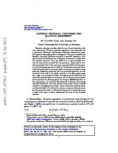
4. The Source-to-Station Path Types In the third generation of regression studies of spectral amplitudes in the 1990s, a new term (Lee et al., 1995; Lee and Trifunac, 1995a, 1995b), r, 0 ≤ r ≤ 1 (or 100r, as a percentage) was introduced. In this, r is the ratio (or percentage) of wave path through geological basement rock relative to the total path, measured along the surface from the earthquake epicenter to the recording site. Alternately, a generalized path type classification was also used. It describes the characteristic types of wave paths between the sources and stations for the strong-motion data available up to the early 1990s in the western U.S. At that time, due to the limited amount of data, only eight such categories could be identified with a sufficient number of recordings to be included in the regression analyses (see Table 9). Figure 1 shows a schematic representation of the “geometry” of these path types. The eight path types in Figure 1 can further be grouped into four path groups: “1”, “2”, “3”, and “4”, as described in Table 10. Table 9: USC Strong-Motion Group Source-to-Station Path Type Path Type 1 2 3 4 5 6 7 8

Description Sediments-to-sediments (100%) Rock-to-sediments, almost vertically Rock-to-sediments, almost horizontally Rock-to-rock (100%) Rock-to-rock through sediments, almost vertically Rock-to-sediments through rock and sediments, almost vertically Rock-to-sediments through rock and sediments, almost horizontally Rock-to-rock through sediments, almost horizontally

5. The Scaling Equations Only the most recent (the third generation) scaling equations (Lee and Trifunac, 1995a, 1995b) for spectral amplitudes will be illustrated here. A description of the complete set of scaling relations of all three generations can be found in Lee (2002). The following regression equations illustrate the four scaling models. Model (i): Mag-site + soil + % rock path multi-step model

log PSV (T ) =

M + Att (∆, M , T ) + b1 (T ) M + b2 (T ) s + b3 (T )v + b4 (T ) + b5 (T ) M 2 + ∑ i b6( i ) (T ) S6(i ) + ( b70 (T )r + b71 (T )(1 − r ) )R
R  + b6(i ) (T ) S6( i ) + ( b70 (T )r + b71 (T )(1 − r ) )Rmax − ∑ max i  200

(20)

52


Fig. 1 Eight path types from source to recording station Table 10: USC Strong-Motion Group Source-to-Station Path Groups Path Group “1”

Path Types Included 1

“2”

2, 6

“3”

3, 7

“4”

4, 5, 8

Description Earthquake source and recording site within the same sediment Earthquake source in basement rock, recording site almost vertically above Earthquake source in basement rock close to the surface; Recording site on nearby sediment, almost horizontally Earthquake source in basement rock, recording site on the same basement rock, with or without sediments in between

Model (ii): Mag-depth + soil + % rock path multi-step model

log PSV (T ) = M + Att (∆, M , T ) + b1 (T ) M + b2 (T )h + b3 (T )v + b4 (T ) + b5 (T ) M 2 + ∑ i b6( i ) (T ) S6(i ) + ( b70 (T )r + b71 (T )(1 − r ) )R
800 m/s and depth < 75–100 m Soil with shear wave velocity < 800 m/s and depth ~ 100–200 m

58


The Strong-Motion Group at USC first started with a completely different site classification. The first, in the 1970s (Trifunac and Brady, 1975b), was proposed to characterize roughly the geological environment of the recording station, using geologic maps. The geological sites were grouped as shown in Table 6. This geological site classification was intended to be measured in “thousands (not hundreds), of feet, or in kilometers (not meters)”. Thus, this is totally different from the soil classifications later proposed by Boore et al. (1993, 1997) and Abrahamson and Silva (1997), which are for the soil deposits below the surface, measured to only about “a hundred feet (not thousands) or meters (not kilometers)”. In the late 1970s, Trifunac and Lee (1979a) refined their site classification and used the “depth of sedimentary deposits beneath the recording site, h, in km, as a geological site characteristic”. The continuous parameter h, and the discrete geological classification s, were subsequently both used at USC in the second and third generations of regression analyses in the 1980s and 1990s. This was the trend in the 1980s—the groups of Boore, Abrahamson, and Ambraseys were all using the surface soil information as a site characteristic, while the Strong-Motion Group at USC was using the geological information below the surface and surrounding the site. In the 1990s, the above differences in site classification and their effects on spectral amplitudes were addressed in the third generation analyses of spectral regressions, in the reports by the Strong-Motion Group at USC (Lee and Trifunac, 1993, 1995a, 1995b; Lee et al., 1995). It is conjectured that the geological characteristics below a site affect the long-to-intermediate periods, or small-to-intermediate frequencies of waves arriving at the site, while the surface soil characteristic at a site affects the short periods (high frequencies) of motions. In the third generation of regressions at USC, two additional parameters were introduced to characterize the local soil site in addition to the geological site effects. The first one is the local soil type, sL , representative of the top 100~200 m beneath the surface (Trifunac, 1990a), defined as in Table 7. A second parameter used was the average soil velocity, VL , in the top 30 m beneath the surface. This is the same parameter as was used by Boore et al. (1994a, 1994b) in their revised site characterization. When this information was not available, a soil velocity type, ST , was adopted, defined as in Table 8. In each case, an indicator variable representing the velocity type is assigned. Thus, the Strong-Motion Group at USC is the only group that has used both geological and soil site classifications in their latest generation of regressions of spectral amplitudes. They argued that both classifications must be included “simultaneously” in the characterization of site-specific spectra because ignoring the local geological conditions may lead to exaggerated factors “representing” the local soil conditions. A study of the response spectral amplitudes of recorded strong motions in California (Lee and Trifunac, 1995b) concluded that the A, B, C, and D local soil classification based only on the average shear wave velocity in the top 30 m, as proposed by Boore et al. (1993), becomes statistically insignificant when used as a third parameter simultaneously with the soil ( sL = 0, 1 and 2) and geological (s = 0, 1 and 2) classifications. This suggests that when the depth of the soil deposit at a site is included in the soil classification, this will out-perform the scaling equations based only on the soil information close to the surface. Finally, we note that the systematic gathering of many of these site soil parameters is often very expensive, difficult, and time consuming, but the geological site description in terms of s = 0, 1 and 2 is simple and easy to perform. The site characterizations used in the spectral regressions in the 1990s for the four groups are summarized in Tables 18(a) and 18(b). Table 18(a): Comparison of Soil Site Characterizations Used by the Four Groups Soil Classification Site Class Soil Velocity average 30 m VL Boore et al. (1993) A, B, C, D Abrahamson and Silva (1997) — A, B, C, D, E Ambraseys et al. (1996, 2005a, 2005b) R, A, S, L — sL : 0, 1, 2 average 30 m VL Lee and Trifunac (1995a, 1995b) Group

Reference Table 1 Table 4 Table 5 Table 7


59

Table 18(b): Comparison of Geological Site Characterizations Used by the Four Groups Geological Classification Site, s Alluvial Depth, h Boore et al. (1993) No No Abrahamson and Silva (1997) No No Ambraseys et al. (1996, 2005a, 2005b) No No Lee and Trifunac (1995a, 1995b) Yes Yes (see Table 6) Group

4. Distance Definition Used in Attenuation Relations In the work of Boore et al. (1993), BJF93, the epicentral distance term used, r, is defined as

r = d 2 + h 2 , where d is the measured epicentral distance in km from the earthquake source to the site, and h is a fictitious depth to be determined. Instead of using the actual measured depth of the earthquake source, Boore et al. (1993) treated h as an unknown parameter to be determined by regression. They first used the attenuation term, b4 r + b5 ln r , in their regression equation, but this was subsequently replaced by b5 ln r . It was pointed out that a regression including the b4 r term resulted in values of b4 greater than zero, which would lead to unreasonable behavior at large distances, and so the term was deleted. The remaining term, b5 ln r , is thus the only term used by Boore et al. (1993, 1997) to characterize the attenuation of the spectral amplitudes from the source to the recording site. In the work of Abrahamson and Silva (1997), the distance introduced by Idriss (1991) and Sadigh et al. (1993)—namely, rrup , is the closest distance from the site to the rupture plane. The distance term is 2 + c42 , which is the same as in Boore et al. (1993), where c4 is again a fictitious term to be then R = rrup

determined by regression. Unlike Boore et al. (1993), where the term c4 is interpreted as a fictitious depth term, Abrahamson and Silva (1997) pointed out that in their model the rupture distance rrup may include the depth for dipping faults and for faults that do not reach the surface. It is not clear if c4 can be interpreted as a fictitious depth, but it is included in their distance definition. The attenuation term used is [ a3 + a13 ( M − c1 )] ln R , which is similar to that used by Boore et al. (1993), except that the coefficient is taken to be dependent upon earthquake magnitude, M. From the seismological and earthquake engineering points of view, the definition of the distance from the earthquake source to the site is not as simple as it may seem. This is because the earthquake source is not a point but a three-dimensional surface, which is often empirically correlated with the magnitude and size of the earthquake. To execute a regression analysis, one has to decide on how to define a distance between a rupture surface area and a recording site. The attenuation of the spectral amplitudes is, thus, even more complicated because the attenuation will also depend upon the frequency of the motions. In the 1980s, Trifunac and Lee (1985a, 1985b) developed the first frequency-dependent attenuation function, Att (∆, M , T ) (see Equation (16)), a function of the “representative” distance ∆ from the source to the site, for magnitude M and period T of strong motion. For a complete, detailed description of this function, the reader is referred to the above references. Here, ∆ is the source-to-station distance of Gusev (1983), selected to include the rupture size of the earthquake (see Equation (17)). In the 1990s, Lee and Trifunac (1990) refined and modified the attenuation function to the form given in Equation (18). This attenuation function aims to account for the complicated nature of the attenuation from the rupture area to the site and is magnitude-, period-, and distance-dependent. Compared with the works of the other three groups—Boore et al. (1993, 1997), Abrahamson and Silva (1997), and Ambraseys et al. (1996)— this is a more detailed description of the attenuation from the source to the site. 5. Differences between the Models: Fault Type and Path Type Boore et al. (1994a, 1994b, 1997), in their updated regression equation, introduced an earthquakefault term (see Equation (3)), as an indicator variable, which defines a constant term, one each for strikeslip, reverse-slip, and unknown-slip earthquakes. This distinction of ground motions that result from

60


strike-slip and reverse-slip faults is a feature that has been studied by others as well (Idriss, 1991; Sadigh et al., 1993; Boore et al., 1993, 1997; Campell and Bozorgnia, 1994; Abrahamson and Silva, 1997). Abrahamson and Silva (1997) introduced a similar term in their regression equation, which they called the style-of-faulting factor, Ff 3 ( M ) , where F is the fault type. It is 1 for reverse, 0.5 for reverse/oblique, and 0 otherwise, and f3 ( M ) is as defined in Equation (6) and fitted for each period T. They, thus, allowed for magnitude and period dependence of the faulting factor. Following Somerville and Abrahamson (2000), they introduced another term to account for the differences in motions from the hanging wall and foot wall of dipping faults; they called this term, f 4 ( M , rrup ) , as the “hanging wall effect” (see Equations (7)-(9)). Ambraseys et al. (1996) did not consider any fault-type parameters in their regression. Ambraseys et al. (2005a, 2005b) did include the fault mechanism terms in their regression equations, as in Boore et al. (1994a, 1994b, 1997). The above indicates that different fault geometries and slip directions could generate different motions at the site, which no one would dispute. If the motions that originate from the fault travel directly to the site without scattering and diffraction, the resulting motions at the site should depend upon the type of faulting and the type of motions at the source. In reality, however, the waves will not travel directly from the source to the site because the medium between the source and the site is almost always very irregular. The waves arriving at the site are thus a combination of waves traveling between different parts of the source and the site along multiple paths, and, therefore, they have undergone significant changes as a result of scattering and diffraction along the path. The arriving signals, besides being attenuated, can thus be very different in phase and amplitude from those at the source. It may be argued and conjectured that such source and fault mechanism factors may have influence mainly on the near-source records and, hence, on the resulting spectra. Further away from the source with increasing distance, such kind of influence may become weaker and weaker. Up till now, there are very few near-field records available in the database worldwide. In the future when more near-field records become available, the question of whether to include a source-mechanism term in regression will be determined by the data. The strong-motion group at USC thus far did not consider earthquake fault-type terms in their regression. Lee and Trifunac (1993, 1995a, 1995b), and Lee et al. (1995) conjectured that, instead, the spectral motions are more dependent on the complicated path between the source and the site. They introduced a generalized path type classification, which describes the different types of wave paths between the source and stations (see Figure 1). As confirmed by the regressions, the path types are significant factors for the resulting motions at the site. Therefore, a new term (Lee et al., 1995a, 1995b), r, with 0 ≤ r ≤ 1 (or 100r, in percentage) was introduced. r is the ratio (or percentage) of wave path through geological basement rock to the total path, measured along the surface from the earthquake epicenter to the recording site. In summary, the use of fault type and path type parameters in the regressions of the four different group is as given in Table 19. Table 19: Fault Type versus Source-to-Station Path Type Group Fault Type Source-to-Station Path Type Boore et al. (1993) Yes No Abrahamson and Silva (1997) Yes No Ambraseys et al. (1996) No No Ambraseys et al. (2005a, 2005b) Yes No Lee and Trifunac (1995a, 1995b) No Yes


61

6. Other Differences between the Models 6.1 Frequency Band of Analysis One additional difference among the various studies of spectral amplitudes has to do with the period range of data in the regression. As noted by many in this field (Trifunac, 2005), the spectral amplitudes are available only for a limited frequency range. This is because the input acceleration data recorded by analog instruments are affected by the recording and digitization noise (Lee et al., 1982). In the 60’s and early 70’s, the digitization process had to be performed manually. In fact, up to 1975, all the recorded accelerograms from the 1933 Long Beach to the 1971 San Fernando earthquakes were processed in this way. The digitized data was not available at many points per second, and the high frequency data beyond 25 Hz (< 0.04 s) was out of reach. At the long period end, the Fourier and spectral data were dependent on the amplitudes of the recorded acceleration, i.e., more dependent on the magnitude of the earthquake, the location of the recording site relative to the earthquake source, and the level of digitization noise associated with the frequency content of the input data. Figure 2 (Lee, 2002) is the PSV spectra for 5% damping and 0.5 probability of exceedance for a site at epicentral distance R = 10 km and on rock (h = 0), the source at depth H = 5 km, and for magnitudes M = 4, 5, 6 and 7. It shows the plot of the usable frequency range of the spectral amplitudes for various amplitudes of the recorded data. The figure shows that the uniformly processed high quality strong-motion data is available at periods from 0.04 second (at or below 25 Hz) up to several seconds, and no more than 10 s (or no less than 0.10 Hz). The figure also indicates the domain (see the lightly shaded area) where the empirical scaling equation can be used.

2 Extrapolated PSV Spectra Trifunac(1995a)

Domain where Empirical Scaling Equations Apply Cut-off fraquencies fc0 = 1 / T(N c)

1

M= 8

Trifunac(1995b)

M= 7

0 M= 6

-1 M= 5

M= 4

Digitization Noise

-2 -2

-1

0 Log (frequency) - Hz

1

Fig. 2 PSV spectra for 5% damping (from Lee (2002))

2

62


This area is bounded by the spectra for M = 4 and M = 7, and is between the period T = 0.04 s and the cut-off period, TC , increasing from TC = 0.90 s for M = 3 and 4 to TC = 7.5 s for M = 7 (Trifunac, 1993a). In the figure, the dark shaded zone, extending from PSV ~ 0.1 in/s around T = 0.04 s to PSV ~ 1 in/s around T = 10.0 s, represents the amplitudes of the recording and processing noise (Trifunac and Todorovska, 2001a). In many engineering applications, the spectral amplitudes need to be specified in a broad frequency band, which is broader than the available band shown above, where the empirical regression equations are valid. Trifunac (1993a, 1993b, 1994a) presented a method for extension of the regression equations of spectral amplitudes to periods at both ends, namely, to the periods beyond just several seconds, and to periods shorter than 0.04 s. 6.2 Component Orientation: Horizontal and Vertical Response Spectra The regression equations of Boore et al. (1997) (see Equations (1) and (2)) have no terms indicating the component orientation of the spectral amplitudes. This is because they considered only the response spectra from the two horizontal components of recorded acceleration at each site. In a similar fashion, Ambraseys et al. (1996) did the regression analyses only on the response spectra from the horizontal components of motions. Abrahamson and Silva (1997) did perform the regression analyses for both the horizontal and vertical response spectra. The vertical components use the same functional form and multiple step procedure as for the horizontal components. The authors listed the coefficients for the horizontal and vertical components in their work. Since the regression procedure is performed separately for the horizontal and vertical components at each period, the coefficients for them are different at each period, even though the scaling equations used have the same form for both components. This means that the dependence of spectral amplitudes on magnitude, distance, local site effects and fault type is different for the horizontal and vertical components in their regression model. Ambraseys et al. (2005a, 2005b), as in Abrahamson and Silva (1997), considered the horizontal and vertical response spectra in separate equations. The strong-motion group at USC considered both the horizontal and vertical components of response spectra in all their studies, the only difference being that the regression for both the horizontal and vertical components were not performed separately, but together simultaneously in one equation (see Equations (19)–(23)). In each of the scaling model, the horizontal and vertical components were differentiated by the term, b3 (T )v, where v = 0 for the horizontal component, and v = 1 for the vertical component. Since both of the components use the same scaling equation, the dependence of the spectral amplitudes on magnitude, distance, path type and site effects are the same for both the horizontal and vertical components of each recorded motion. The only difference between them is just one scaling factor b3 (T )v. This approach is more physical since the horizontal and vertical motions of the recorded accelerations are just components of the total resultant motion at the site. They should thus have the same dependence on magnitude, distance, path type and site effects. A summary of the above is given in Table 20. Table 20: Summary of Regression Works on Horizontal and Vertical Components of Motions Group Boore et al. (1993) Abrahamson and Silva (1997) Ambraseys et al. (1996) Ambraseys et al. (2005a, 2005b) Lee and Trifunac (1995a, 1995b)

Horizontal Vertical Together? Yes No — Yes Yes No Yes No — Yes Yes No Yes Yes Yes

6.3 Scaling in Terms of Earthquake Intensity Of the four groups, the strong-motion group at USC is the only group that has developed scaling equations of response spectra in terms of earthquake intensity. The other three groups used only earthquake magnitude in their regression analyses.


63

ACKNOWLEDGEMENTS The author would like to thank the anonymous reviewers for their critical and constructive comments that resulted in numerous improvements in the final version of this paper. REFERENCES 1. Abrahamson, N.A. and Silva, W.J. (1997). “Empirical Response Spectral Attenuation Relations for Shallow Crustal Earthquakes”, Seismological Research Letters, Vol. 68, No. 1, pp. 94–127. 2. Ambraseys, N.N., Simpson, K.A. and Bommer, J.J. (1996). “Prediction of Horizontal Response Spectra in Europe”, Earthquake Engineering & Structural Dynamics, Vol. 25, No. 4, pp. 371–400. 3. Ambraseys, N.N., Douglas, J., Sarma, S.K. and Smit, P.M. (2005a). “Equations for the Estimation of Strong Ground Motions from Shallow Crustal Earthquakes Using Data from Europe and the Middle East: Horizontal Peak Ground Acceleration and Spectral Acceleration”, Bulletin of Earthquake Engineering, Vol. 3, No. 1, pp. 1–53. 4. Ambraseys, N., Douglas, J., Sarma, S.K. and Smit, P. (2005b). “Equations for the Estimation of Strong Ground Motions from Shallow Crustal Earthquakes Using Data from Europe and the Middle East: Vertical Peak Ground Acceleration and Spectral Acceleration”, Bulletin of Earthquake Engineering, Vol. 3, No. 1, pp. 55–73. 5. Amini, A. and Trifunac, M.D. (1985). “Statistical Extension of Response Spectrum Superposition”, International Journal of Soil Dynamics and Earthquake Engineering, Vol. 4, No. 2, pp. 54–63. 6. Anderson, J.G., Trifunac, M.D., Teng, T.L., Amini, A. and Moslem, K. (1981). “Los Angeles Vicinity Strong Motion Accelerograph Network”, Report CE 81-04, University of Southern California, Los Angeles, U.S.A. 7. Biot, M.A. (1932). “Transient Oscillations in Elastic Systems”, Ph.D. Thesis No. 259, Aeronautics Department, California Institute of Technology, Pasadena, U.S.A. 8. Biot, M.A. (1933). “Theory of Elastic Systems Vibrating under Transient Impulse with an Application to Earthquake-Proof Buildings”, Proceedings of the National Academy of Sciences of the United States of America, Vol. 19, No. 2, pp. 262–268. 9. Biot, M.A. (1934). “Theory of Vibration of Buildings during Earthquake”, Zeitschrift für Angewandte Matematik und Mechanik, Vol. 14, No. 4, pp. 213–223. 10. Boore, D.M., Joyner, W.B. and Fumal, T.E. (1993). “Estimation of Response Spectra and Peak Accelerations from Western North American Earthquakes: An Interim Report”, Open-File Report 93509, United States Geological Survey, Denver, U.S.A. 11. Boore, D.M., Joyner, W.B. and Fumal, T.E. (1994a). “Estimation of Response Spectra and Peak Accelerations from Western North American Earthquakes: An Interim Report, Part 2”, Open-File Report 94-127, United States Geological Survey, Denver, U.S.A. 12. Boore, D.M., Joyner, W.B. and Fumal, T.E. (1994b). “Ground Motion Estimates for Strike- and Reverse-Slip Faults”, Insert in “Estimation of Response Spectra and Peak Accelerations from Western North American Earthquakes: An Interim Report, Part 2 (by D.M. Boore, W.B. Joyner and T.E. Fumal)” for the Southern California Earthquake Center, Open-File Report 94-127, United States Geological Survey, Denver, U.S.A. 13. Boore, D.M., Joyner, W.B. and Fumal, T.E. (1997). “Equations for Estimating Horizontal Response Spectra and Peak Acceleration from Western North American Earthquakes: A Summary of Recent Work”, Seismological Research Letters, Vol. 68, No. 1, pp. 128–153. 14. Campbell, K.W. and Bozorgnia, Y. (1994). “Near-Source Attenuation of Peak Horizontal Acceleration from Worldwide Accelerograms Recorded from 1957 to 1993”, Proceedings of the 5th National Conference of Earthquake Engineering, Chicago, U.S.A., Vol. 1, pp. 283–292. 15. Chandrasekaran, A.R., Das, J.D., Trifunac, M.D., Todorovska, M.I. and Lee, V.W. (1993). “Strong Earthquake Ground Motion Data in EQINFOS for India: Part IB”, Report CE 93-04, University of Southern California, Los Angeles, U.S.A. 16. Converse, A.M. and Brady, A.G. (1992). “BAP, Basic Strong-Motion Accelerogram Processing Software; Version 1.0”, Open-File Report 92-296A, United States Geological Survey, Denver, U.S.A.

64


17. Das, S., Gupta, I.D. and Gupta, V.K. (2002). “A New Attenuation Model for North-East India”, Proceedings of the 12th Symposium on Earthquake Engineering, Roorkee, pp. 151–158. 18. Grazier, V.M. (1979). “Determination of the True Ground Displacement by Using Strong Motion Records”, Physics of the Solid Earth, Izvestiya Academy of Sciences, U.S.S.R., Vol. 15, No. 12, pp. 875–885 (English edition published by the American Geophysical Union). 19. Gupta, I.D. and Trifunac, M.D. (1988a). “Order Statistics of Peaks in Earthquake Response”, Journal of Engineering Mechanics, ASCE, Vol. 114, No. 10, pp. 1605–1627. 20. Gupta, I.D. and Trifunac, M.D. (1988b). “Attenuation of Intensity with Epicentral Distance in India”, Soil Dynamics and Earthquake Engineering, Vol. 7, No. 3, pp. 162–169. 21. Gupta, I.D. and Trifunac, M.D. (1990a). “Probabilistic Spectrum Superposition for Response Analysis Including the Effects of Soil-Structure Interaction”, Probabilistic Engineering Mechanics, Vol. 5, No. 1, pp. 9–18. 22. Gupta, V.K. and Trifunac, M.D. (1990b). “Response of Multistoried Buildings to Ground Translation and Rocking during Earthquakes”, Probabilistic Engineering Mechanics, Vol. 5, No. 3, pp. 138–145. 23. Gupta, I.D., Rambabu, V. and Joshi, R.G. (1993). “Strong Earthquake Ground Motion Data in EQINFOS for India: Part 1A (edited by M.D. Trifunac, M.I. Todorovska and V.W. Lee)”, Report CE 93-03, University of Southern California, Los Angeles, U.S.A. 24. Gusev, A.A. (1983). “Descriptive Statistical Model of Earthquake Source Radiation and Its Application to an Estimation of Short-Period Strong Motion”, Geophysical Journal of the Royal Astronomical Society, Vol. 74, No. 3, pp. 787–808. 25. Hudson, D.E., Trifunac, M.D. and Brady, A.G. (1970). “Strong-Motion Earthquake Accelerograms, Digitized and Plotted Data, Vol. I”, Report EERL 70-20, California Institute of Technology, Pasadena, U.S.A. 26. Hudson, D.E., Trifunac, M.D., Brady, A.G. and Vijayaraghavan, A. (1971). “Strong-Motion Earthquake Accelerograms, II, Corrected Accelerograms and Integrated Velocity and Displacement Curves”, Report EERL 71-50, California Institute of Technology, Pasadena, U.S.A. 27. Hudson, D.E., Trifunac, M.D. and Brady, A.G. (1972a). “Strong-Motion Accelerograms, III, Response Spectra”, Report EERL 72-80, California Institute of Technology, Pasadena, U.S.A. 28. Hudson, D.E., Trifunac, M.D., Udwadia, F.E. and Vijayaraghavan, A. (1972b). “Strong-Motion Earthquake Accelerograms, IV, Fourier Spectra”, Report EERL 72-100, California Institute of Technology, Pasadena, U.S.A. 29. Idriss, I.M. (1991). “Selection of Earthquake Ground Motions at Rock Sites”, Report prepared for National Institute of Standards and Technology, Department of Civil Engineering, University of California, Davis, U.S.A. 30. Jordanovski, L.R., Lee, V.W., Manic, M.I., Olumceva, T., Sinadinovski, C., Todorovska, M.I. and Trifunac, M.D. (1987). “Strong Earthquake Ground Motion Data in EQINFOS: Yugoslavia, Part I”, Report CE 87-05, University of Southern California, Los Angeles, U.S.A. 31. Jordanovski, L.R., Todorovska, M.I. and Trifunac, M.D. (1992a). “Total Loss in a Building Exposed to Earthquake Hazard, Part I: The Model”, European Earthquake Engineering, Vol. VI, No. 3, pp. 14– 25. 32. Jordanovski, L.R., Todorovska, M.I. and Trifunac, M.D. (1992b). “Total Loss in a Building Exposed to Earthquake Hazard, Part II: A Hypothetical Example”, European Earthquake Engineering, Vol. VI, No. 3, pp. 26–32. 33. Joyner, W.B. and Boore, D.M. (1981). “Peak Horizontal Acceleration and Velocity from StrongMotion Records Including Records from the 1979 Imperial Valley, California, Earthquake”, Bulletin of the Seismological Society of America, Vol. 71, No. 6, pp. 2011–2038. 34. Joyner, W.B. and Boore, D.M. (1982). “Prediction of Earthquake Response Spectra”, Open-File Report 82-977, United States Geological Survey, Denver, U.S.A. 35. Joyner, W.B. and Boore, D.M. (1993). “Methods for Regression Analysis of Strong-Motion Data”, Bulletin of the Seismological Society of America, Vol. 83, No. 2, pp. 469–487.


65

36. Kanamori, H. (1977). “The Energy Release in Great Earthquakes”, Journal of Geophysical Research, Vol. 82, No. 20, pp. 2981–2988. 37. Lee, V.W. (1989). “Empirical Scaling of Pseudo Relative Velocity Spectra of Recorded Strong Earthquake Motion in Terms of Magnitude and Both Local Soil and Geologic Site Classifications”, Earthquake Engineering and Engineering Vibrations, Vol. 9, No. 3, pp. 9–29. 38. Lee, V.W. (1990). “Scaling PSV Spectra in Terms of Site Intensity, and Both Local Soil and Geological Site Classifications”, European Earthquake Engineering, Vol. IV, No. 1, pp. 3–12. 39. Lee, V.W. (1991). “Correlation of Pseudo Relative Velocity Spectra with Site Intensity, Local Soil Classification and Depth of Sediments”, Soil Dynamics and Earthquake Engineering, Vol. 10, No. 3, pp. 141–151. 40. Lee, V.W. (1993). “Scaling PSV from Earthquake Magnitude, Local Soil, and Geologic Depth of Sediments”, Journal of Geotechnical Engineering, ASCE, Vol. 119, No. 1, pp. 108–126. 41. Lee, V.W. (1997). “Discussion: Prediction of Horizontal Response Spectra in Europe", Earthquake Engineering & Structural Dynamics, Vol. 26, No. 2, pp. 289–293. 42. Lee, V.W. (2002). “Empirical Scaling of Strong Earthquake Ground Motion—Part I: Attenuation and Scaling of Response Spectra”, ISET Journal of Earthquake Technology, Vol. 39, No. 4, pp. 219–254. 43. Lee, V.W. and Manic, M. (1994). “Empirical Scaling of Response Spectra in Former Yugoslavia”, Proceedings of the Tenth European Conference on Earthquake Engineering, Vienna, Austria, Vol. IV, pp. 2567–2572. 44. Lee, V.W. and Trifunac, M.D. (1979) “Automatic Digitization and Processing of Strong-Motion Accelerograms, Part II: Computer Processing of Accelerograms”, Report CE 79-15 II, University of Southern California, Los Angeles, U.S.A. 45. Lee, V.W. and Trifunac, M.D. (1984). “Current Developments in Data Processing of Strong-Motion Accelerograms”, Report CE 84-01, University of Southern California, Los Angeles, U.S.A. 46. Lee, V.W. and Trifunac, M.D. (1985). “Attenuation of Modified Mercalli Intensity for Small Epicentral Distances in California”, Report CE 85-01, University of Southern California, Los Angeles, U.S.A. 47. Lee, V.W. and Trifunac, M.D. (1990). “Automatic Digitization and Processing of Accelerograms Using PC”, Report CE 90-03, University of Southern California, Los Angeles, U.S.A. 48. Lee, V.W. and Trifunac, M.D. (1992). “Frequency Dependent Attenuation of Strong Earthquake Ground Motion in Yugoslavia”, European Earthquake Engineering, Vol. VI, No. 1, pp. 3–13. 49. Lee, V.W. and Trifunac, M.D. (1993). “Empirical Scaling of Fourier Amplitude Spectra in Former Yugoslavia”, European Earthquake Engineering, Vol. VII, No. 2, pp. 47–61. 50. Lee, V.W. and Trifunac, M.D. (1995a). “Frequency Dependent Attenuation Function and Fourier Amplitude Spectra of Strong Earthquake Ground Motion in California”, Report CE 95-03, Department of Civil Engineering, University of Southern California, Los Angeles, California, 355pp. 51. Lee, V.W. and Trifunac, M.D. (1995b). “Pseudo Relative Velocity Spectra of Strong Earthquake Ground Motion in California”, Report No. CE 95-04, University of Southern California, Los Angeles, U.S.A. 52. Lee, V.W., Trifunac, M.D. and Amini, A. (1982). “Noise in Earthquake Accelerograms”, Journal of the Engineering Mechanics Division, Proceedings of ASCE, Vol. 108, No. EM6, pp. 1121–1129. 53. Lee, V.W., Trifunac, M.D., Todorovska, M.I. and Novikova, E.I. (1995). “Empirical Equations Describing Attenuation of the Peaks of Strong Ground Motion, in Terms of Magnitude, Distance, Path Effects, and Site Conditions”, Report CE 95-02, University of Southern California, Los Angeles, U.S.A. 54. Nenov, D., Georgiev, G., Paskaleva, I., Lee, V.W. and Trifunac, M.D. (1990). “Strong Earthquake Ground Motion Data in EQINFOS: Accelerograms Recorded in Bulgaria between 1981 and 1987”, Report CE 90-02, Bulgarian Academy of Sciences, Sofia, Bulgaria, and University of Southern California, Los Angeles, U.S.A. 55. Novikova, E.I., Todorovska, M.I. and Trifunac, M.D. (1993). “A Preliminary Study of the Duration of Strong Earthquake Ground Motion on the Territory of Former Yugoslavia”, Report CE 93-09, University of Southern California, Los Angeles, U.S.A.

66


56. Press, W.H., Teukolsky, S.A., Vetterling, W.T. and Flannery, B.P. (1992). “Numerical Recipes”, Cambridge University Press, London, U.K. 57. Rabiner, L.R. and Gold, B. (1975). “Theory and Application of Digital Signal Processing”, PrenticeHall, Englewood Cliffs, U.S.A. 58. Richter, C.F. (1958). “Elementary Seismology”, W.H. Freeman & Company, San Francisco, U.S.A. 59. Sadigh, K., Chang, C.-Y., Abrahamson, N.A., Chiou, S.J. and Power, M. (1993). “Specification of Long Period Motions: Updated Attenuation Relations for Rock Site Conditions and Adjustment Factors for Near-Fault Effects” in “Proceedings of a Seminar on Seismic Isolation, Passive Energy Dissipation and Active Control”, Report ATC-17-1, Applied Technology Council, Redwood City, California, U.S.A. 60. Seed, H.B., Ugas, C. and Lysmer, J. (1974). “Site-Dependent Spectra for Earthquake-Resistant Design”, Report UCB/EERC-74/12, University of California, Berkeley, U.S.A. 61. Shebalin, N.V., Karnik, V. and Hadžievski, D. (editors) (1974). “Catalogue of Earthquakes (Part I, 1901–1970; Part II, Prior to 1901)”, UNDP/UNESCO Survey of the Seismicity of the Balkan Region, UNESCO, Skopje, Yugoslavia. 62. Somerville, P. and Abrahamson, N. (2000). “Prediction of Ground Motions for Thrust Earthquakes”, Data Utilization Report CSMIP/00-01, California Department of Conservation, Sacramento, U.S.A. 63. Sunder, S.S. and Conner, J.J. (1982). “A New Procedure for Processing Strong-Motion Earthquake Signals”, Bulletin of the Seismological Society of America, Vol. 72, No. 2, pp. 643–661. 64. Todorovska, M.I. (1994a). “Order Statistics of Functionals of Strong Motion”, Soil Dynamics and Earthquake Engineering, Vol. 13, No. 3, pp. 149–161. 65. Todorovska, M.I. (1994b). “Comparison of Response Spectrum Amplitudes from Earthquakes with Lognormally and Exponentially Distributed Return Period”, Soil Dynamics and Earthquake Engineering, Vol. 13, No. 2, pp. 97–116. 66. Todorovska, M.I. (1995). “A Note on Distribution of Amplitudes of Peaks in Structural Response Including Uncertainties of the Exciting Ground Motion and of the Structural Model”, Soil Dynamics and Earthquake Engineering, Vol. 14, No. 3, pp. 211–217. 67. Trifunac, M.D. (1972). “A Note on Correction of Strong-Motion Accelerograms for Instrument Response”, Bulletin of the Seismological Society of America, Vol. 62, No. 1, pp. 401–409. 68. Trifunac, M.D. (1973). “Analysis of Strong Earthquake Ground Motion for Prediction of Response Spectra”, Earthquake Engineering & Structural Dynamics, Vol. 2, No. 1, pp. 59–69. 69. Trifunac, M.D. (1976a). “Preliminary Analysis of the Peaks of Strong Earthquake Ground Motion— Dependence of Peaks on Earthquake Magnitude, Epicentral Distance, and Recording Site Conditions”, Bulletin of the Seismological Society of America, Vol. 66, No. 1, pp. 189–219. 70. Trifunac, M.D. (1976b). “Preliminary Empirical Model for Scaling Fourier Amplitude Spectra of Strong Ground Acceleration in Terms of Earthquake Magnitude, Source-to-Station Distance, and Recording Site Conditions”, Bulletin of the Seismological Society of America, Vol. 66, No. 4, pp. 1343–1373. 71. Trifunac, M.D. (1976c). “A Note on the Range of Peak Amplitudes of Recorded Accelerations, Velocities and Displacements with Respect to the Modified Mercalli Intensity”, Earthquake Notes, Vol. 47, No. 1, pp. 9–24. 72. Trifunac, M.D. (1977a). “Statistical Analysis of the Computed Response of Structural Response Recorders (S.R.R.) for Accelerograms Recorded in the United States of America”, Proceedings of the Sixth World Conference on Earthquake Engineering, New Delhi, Vol. III, pp. 2956–2961. 73. Trifunac, M.D. (1977b). “Forecasting the Spectral Amplitudes of Strong Earthquake Ground Motion”, Proceedings of the Sixth World Conference on Earthquake Engineering, New Delhi, Vol. I, pp. 139–152. 74. Trifunac, M.D. (1977c). “An Instrumental Comparison of the Modified Mercalli (M.M.I.) and Medvedev-Karnik-Sponheuer (M.K.S.) Intensity Scales”, Proceedings of the Sixth World Conference on Earthquake Engineering, New Delhi, Vol. I, pp. 715–721.


67

75. Trifunac, M.D. (1977d). “Uniformly Processed Strong Earthquake Ground Accelerations in the Western United States of America for the Period from 1933 to 1971: Pseudo Relative Velocity Spectra and Processing Noise”, Report CE 77-04, University of Southern California, Los Angeles, U.S.A. 76. Trifunac, M.D. (1978). “Response Spectra of Earthquake Ground Motion”, Journal of the Engineering Mechanics Division, Proceedings of ASCE, Vol. 104, No. EM5, pp. 1081–1097. 77. Trifunac, M.D. (1979). “Preliminary Empirical Model for Scaling Fourier Amplitude Spectra of Strong Motion Acceleration in Terms of Modified Mercalli Intensity and Geologic Site Conditions”, Earthquake Engineering & Structural Dynamics, Vol. 7, No. 1, pp. 63–74. 78. Trifunac, M.D. (1988). “Seismic Microzonation Mapping via Uniform Risk Spectra”, Proceedings of the Ninth World Conference on Earthquake Engineering, Tokyo-Kyoto, Japan, Vol. VII, pp. 75–80. 79. Trifunac, M.D. (1989a). “Dependence of Fourier Spectrum Amplitudes of Recorded Strong Earthquake Accelerations on Magnitude, Local Soil Conditions and on Depth of Sediments”, Earthquake Engineering & Structural Dynamics, Vol. 18, No. 7, pp. 999–1016. 80. Trifunac, M.D. (1989b). “Empirical Scaling of Fourier Spectrum Amplitudes of Recorded Strong Earthquake Accelerations in Terms of Magnitude and Local Soil and Geologic Conditions”, Earthquake Engineering and Engineering Vibration, Vol. 9, No. 2, pp. 23–44. 81. Trifunac, M.D. (1989c). “Scaling Strong Motion Fourier Spectra by Modified Mercalli Intensity, Local Soil and Geologic Site Conditions”, Structural Engineering/Earthquake Engineering, JSCE, Vol. 6, No. 2, pp. 217–224. 82. Trifunac, M.D. (1989d). “Threshold Magnitudes Which Exceed the Expected Ground Motion during the Next 50 Years in a Metropolitan Area”, Geofizika, Vol. 6, No. 1, pp. 1–12. 83. Trifunac, M.D. (1990a). “How to Model Amplification of Strong Earthquake Motions by Local Soil and Geologic Site Conditions”, Earthquake Engineering & Structural Dynamics, Vol. 19, No. 6, pp. 833–846. 84. Trifunac, M.D. (1990b). “A Microzonation Method Based on Uniform Risk Spectra”, Soil Dynamics and Earthquake Engineering, Vol. 9, No. 1, pp. 34–43. 85. Trifunac, M.D. (1991a). “Empirical Scaling of Fourier Spectrum Amplitudes of Recorded Strong Earthquake Accelerations in Terms of Modified Mercalli Intensity, Local Soil Conditions and Depth of Sediments”, Soil Dynamics and Earthquake Engineering, Vol. 10, No. 1, pp. 65–72. 86. Trifunac, M.D. (1991b). “MLSM”, Soil Dynamics and Earthquake Engineering, Vol. 10, No. 1, pp. 17– 25. 87. Trifunac, M.D. (1993a). “Long Period Fourier Amplitude Spectra of Strong Motion Acceleration”, Soil Dynamics and Earthquake Engineering, Vol. 12, No. 6, pp. 363–382. 88. Trifunac, M.D. (1993b). “Broad Band Extension of Fourier Amplitude Spectra of Strong Motion Acceleration”, Report CE 93-01, University of Southern California, Los Angeles, U.S.A. 89. Trifunac, M.D. (1994a). “Fourier Amplitude Spectra of Strong Motion Acceleration: Extension to High and Low Frequencies”, Earthquake Engineering & Structural Dynamics, Vol. 23, No. 4, pp. 389–411. 90. Trifunac, M.D. (1994b). “Q and High-Frequency Strong Motion Spectra”, Soil Dynamics and Earthquake Engineering, Vol. 13, No. 3, pp. 149–161. 91. Trifunac, M.D. (1994c). “Earthquake Source Variables for Scaling Spectral and Temporal Characteristics of Strong Ground Motion”, Proceedings of the Tenth European Conference of Earthquake Engineering, Vienna, Austria, Vol. 4, pp. 2585–2590. 92. Trifunac, M.D. (1994d). “Response Spectra of Strong Motion Acceleration: Extension to High and Low Frequencies”, Proceedings of the Tenth European Conference of Earthquake Engineering, Vienna, Austria, Vol. 1, pp. 203–208. 93. Trifunac, M.D. (1994e). “Broad Band Extension of Pseudo Relative Velocity Spectra of Strong Motion”, Report CE 94-02, University of Southern California, Los Angeles, U.S.A. 94. Trifunac, M.D. (1995a). “Pseudo Relative Velocity Spectra of Earthquake Ground Motion at Long Periods”, Soil Dynamics and Earthquake Engineering, Vol. 14, No. 5, pp. 331–346.

68


95. Trifunac, M.D. (1995b). “Pseudo Relative Velocity Spectra of Earthquake Ground Motion at High Frequencies”, Earthquake Engineering & Structural Dynamics, Vol. 24, No. 8, pp. 1113–1130. 96. Trifunac, M.D. (2005). “The Role of the Brune Spectrum in Earthquake Engineering”, Journal of Seismology and Earthquake Engineering, Vol. 7, No. 2, pp. 63–82. 97. Trifunac, M.D. (2006). “Brief History of Computation of Earthquake Response Spectra”, Soil Dynamics and Earthquake Engineering, Vol. 26, No. 6-7, pp. 501–508. 98. Trifunac, M.D. and Anderson, J.G. (1977). “Preliminary Empirical Models for Scaling Absolute Acceleration Spectra”, Report CE 77-03, University of Southern California, Los Angeles, U.S.A. 99. Trifunac, M.D. and Anderson, J.G. (1978a). “Preliminary Empirical Models for Scaling Pseudo Relative Velocity Spectra”, Report CE 78-04, University of Southern California, Los Angeles, U.S.A. 100. Trifunac, M.D. and Anderson, J.G. (1978b). “Preliminary Models for Scaling Relative Velocity Spectra”, Report CE 78-05, University of Southern California, Los Angeles, U.S.A. 101. Trifunac, M.D. and Anderson, J.G. (1978c). “Estimation of Relative Velocity Spectra”, Proceedings of the Sixth Symposium on Earthquake Engineering, Roorkee, Vol. I, pp. 9–18. 102. Trifunac, M.D. and Brady, A.G. (1975a). “A Study on the Duration of Strong Earthquake Ground Motion”, Bulletin of the Seismological Society of America, Vol. 65, No. 3, pp. 581–626. 103. Trifunac, M.D. and Brady, A.G. (1975b). “On the Correlation of Seismic Intensity Scales with the Peaks of Recorded Strong Ground Motion”, Bulletin of the Seismological Society of America, Vol. 65, No. 1, pp. 139–162. 104. Trifunac, M.D. and Brady, A.G. (1975c). “On the Correlation of Seismoscope Response with Earthquake Magnitude and Modified Mercalli Intensity”, Bulletin of the Seismological Society of America, Vol. 65, No. 2, pp. 307–321. 105. Trifunac, M.D. and Brady, A.G. (1975d). “Correlations of Peak Acceleration, Velocity and Displacement with Earthquake Magnitude, Epicentral Distance and Site Conditions”, Earthquake Engineering & Structural Dynamics, Vol. 4, No. 5, pp. 455–471. 106. Trifunac, M.D. and Brady, A.G. (1975e). “On the Correlation of Peak Accelerations of StrongMotion with Earthquake Magnitude, Epicentral Distance and Site Conditions”, Proceedings of the U.S. National Conference on Earthquake Engineering, Ann Arbor, U.S.A., pp. 43–52. 107. Trifunac, M.D. and Lee, V.W. (1973). “Routine Computer Processing of Strong-Motion Accelerograms”, Report EERL 73-03, California Institute of Technology, Pasadena, U.S.A. 108. Trifunac, M.D. and Lee, V.W. (1978). “Dependence of Fourier Amplitude Spectra of Strong Motion Acceleration on the Depth of Sedimentary Deposits”, Report CE 78-14, University of Southern California, Los Angeles, U.S.A. 109. Trifunac, M.D. and Lee, V.W. (1979a). “Dependence of Pseudo Relative Velocity Spectra of Strong Motion Acceleration on the Depth of Sedimentary Deposits”, Report CE 79-02, University of Southern California, Los Angeles, U.S.A. 110. Trifunac, M.D. and Lee, V.W. (1979b). “Automatic Digitization and Processing of Strong-Motion Accelerograms, Part I: Automatic Digitization”, Report CE 79-15 I, University of Southern California, Los Angeles, U.S.A. 111. Trifunac, M.D. and Lee, V.W. (1980). “Fourier Amplitude Spectra of Strong Motion Acceleration”, The Bulletin of the European Association for Earthquake Engineering, Vol. 6, No. 1, pp. 2–18. 112. Trifunac, M.D. and Lee, V.W. (1985a). “Frequency Dependent Attenuation of Strong Earthquake Ground Motion”, Report CE 85-02, University of Southern California, Los Angeles, U.S.A. 113. Trifunac, M.D. and Lee, V.W. (1985b). “Preliminary Empirical Model for Scaling Fourier Amplitude Spectra of Strong Ground Acceleration in Terms of Earthquake Magnitude, Source to Station Distance, Site Intensity and Recording Site Conditions”, Report CE 85-03, University of Southern California, Los Angeles, U.S.A. 114. Trifunac, M.D and Lee, V.W. (1985c). “Preliminary Empirical Model for Scaling Pseudo Relative Velocity Spectra of Strong Earthquake Accelerations in Terms of Magnitude, Distance, Site Intensity and Recording Site Conditions”, Report CE 85-04, University of Southern California, Los Angeles, U.S.A.


69

115. Trifunac, M.D. and Lee, V.W. (1987). “Direct Empirical Scaling of Response Spectral Amplitudes from Various Site and Earthquake Parameters”, Report NUREG/CR-4903, Vol. 1, United States Nuclear Regulatory Commission, Washington, DC, U.S.A. 116. Trifunac, M.D. and Lee, V.W. (1989a). “Empirical Models for Scaling Fourier Amplitude Spectra of Strong Ground Acceleration in Terms of Earthquake Magnitude, Source to Station Distance, Site Intensity and Recording Site Conditions”, Soil Dynamics and Earthquake Engineering, Vol. 8, No. 3, pp. 110–125. 117. Trifunac, M.D. and Lee, V.W. (1989b). “Empirical Models for Scaling Pseudo Relative Velocity Spectra of Strong Earthquake Accelerations in Terms of Magnitude, Distance, Site Intensity and Recording Site Conditions”, Soil Dynamics and Earthquake Engineering, Vol. 8, No. 3, pp. 126– 144. 118. Trifunac, M.D. and Lee, V.W. (1990). “Frequency Dependent Attenuation of Strong Earthquake Ground Motion”, Soil Dynamics and Earthquake Engineering, Vol. 9, No. 1, pp. 3–15. 119. Trifunac, M.D. and Lee, V.W. (1992). “A Note on Scaling Peak Acceleration, Velocity and Displacement of Strong Earthquake Shaking by Modified Mercalli Intensity (MMI) and Site Soil and Geologic Conditions”, Soil Dynamics and Earthquake Engineering, Vol. 11, No. 2, pp. 101–110. 120. Trifunac, M.D. and Novikova, E.I. (1994). “State of the Art Review of Strong Motion Duration”, Proceedings of the Tenth European Conference on Earthquake Engineering, Vienna, Austria, Vol. 1, pp. 131–140. 121. Trifunac, M.D. and Todorovska, M.I. (1989a). “Attenuation of Seismic Intensity in Albania and Yugoslavia”, Soil Dynamics and Earthquake Engineering, Vol. 18, No. 5, pp. 617–631. 122. Trifunac, M.D. and Todorovska, M.I. (1989b). “Methodology for Selection of Earthquake Design Motions for Important Engineering Structures”, Report CE 89-01, University of Southern California, Los Angeles, U.S.A. 123. Trifunac, M.D. and Todorovska, M.I. (2001a). “A Note on the Useable Range in Accelerographs Recording Translation”, Soil Dynamics and Earthquake Engineering, Vol. 21, No. 4, pp. 275–286. 124. Trifunac, M.D. and Todorovska, M.I. (2001b). “Evolution of Accelerographs, Data Processing, Strong Motion Arrays and Amplitude and Spatial Resolution in Recording Strong Earthquake Motion”, Soil Dynamics and Earthquake Engineering, Vol. 21, No. 6, pp. 537–555. 125. Trifunac, M.D. and Zivcic, M. (1991). “A Note on Instrumental Comparison of the Modified Mercalli Intensity (MMI) in the Western United States and the Mercalli-Cancani-Sieberg (MCS) Intensity in Yugoslavia”, European Earthquake Engineering, Vol. V, No. 1, pp. 22–26. 126. Trifunac, M.D., Udwadia, F.E. and Brady, A.G. (1973). “Analysis of Errors in Digitized StrongMotion Accelerograms”, Bulletin of the Seismological Society of America, Vol. 63, No. 1, pp. 157– 187. 127. Trifunac, M.D., Lee, V.W., Cao, H. and Todorovska, M.I. (1988). “Attenuation of Seismic Intensity in Balkan Countries”, Report CE 88-01, University of Southern California, Los Angeles, U.S.A. 128. Trifunac, M.D., Lee, V.W., Zivcic, M. and Manic, M. (1991). “On the Correlation of MercalliCancani-Sieberg Intensity Scale in Yugoslavia with the Peaks of Recorded Strong Earthquake Ground Motion”, European Earthquake Engineering, Vol. V, No. 1, pp. 27–33. 129. Youngs, R.R. (1993). “Soil Amplification and Vertical to Horizontal Ratios for Analysis of Strong Motion Data from Active Tectonic Regions” in “Guidelines for Determining Design Basis Ground Motions, Vol. 2: Appendices for Ground Motion Estimation”, Report TR-102293, Electric Power Research Institute, Palo Alto, U.S.A.

empirical scaling and regression methods for earthquake strong ... - IITK

empirical scaling and regression methods for earthquake strong ... - IITK

Suggest Documents

A Review on Empirical Likelihood Methods for Regression

Empirical Scaling of Rotational Spectra of Strong ... - CiteSeerX

Empirical Scaling of Rotational Spectra of Strong ... - CiteSeerX

poisson regression with a periodic function - IITK

Quantile Regression using Metaheuristic Algorithms - IITK

Scaling Earthquake Records for Response-History ...

Guidelines for Empirical Vulnerability Assessment - Global Earthquake ...

Fault heterogeneity and earthquake scaling - Semantic Scholar

Methods and Benchmarks for Auto-Scaling ...

Regression Methods and Performance Criteria for

Approximate Bayesian Inference Methods for Regression and ...

Modulus of strong proximinality and continuity of metric projection - IITK

Analytic and Empirical Methods Empirical Evaluations: Validity

Asymptotic scaling from strong coupling

Selecting and Scaling Earthquake Ground Motions for ... - MCEER

Soil Dynamics and Earthquake Engineering Empirical

Bayesian empirical likelihood for quantile regression - arXiv

Selecting and Scaling Earthquake Ground Motions for Performing ...

Scaling Range and Cutoffs in Empirical Fractals

the early entrance of dynamics in earthquake engineering: arturo ... - IITK

Probabilistic Modeling of Earthquake Hazard in Stable Continental - IITK

Methods for Earthquake Analysis - BIBSYS Brage

Athens Earthquake of 7 September 1999: Intensity Measures ... - IITK

Strong Tsunamis in the Mediterranean Sea: A Re-evaluation - IITK