surplus is to increase demand for a product. If price volatility does indeed inhibit demand, as the proponents of dairy compacts argue, the quantity demanded by.
Journal of Agribusiness 18,2(Spring 2000):155S172 © 2000 Agricultural Economics Association of Georgia
Empirical Tests of the Argument that Consumers Value Stable Retail Milk Prices Leigh J. Maynard Existing policy allows interstate dairy compacts if they serve a compelling public interest. Compact supporters argue consumers benefit from retail price stability, but no supporting evidence was found. Milk demand systems were estimated using scanner data and four measures of price volatility. Price volatility defined as forecast errors influenced demand, but did not systematically depress demand. Response was more elastic to unanticipated than anticipated price changes, possibly explaining the higher elasticities often observed in scanner data studies. Key Words: dairy compacts, dairy demand, price instability, scanner data
The 1996 Federal Agriculture Improvement and Reform (FAIR) Act allowed the formation of the Northeast Dairy Compact only if the Secretary of Agriculture found a compelling public interest justifying the compact’s existence. In the current debates about whether to extend the Northeast Dairy Compact and establish a Southern Dairy Compact, some of the most contentious issues involve the impact of dairy compacts on consumer welfare. Proponents of the compact often argue that, although higher retail prices are likely, consumers will benefit from more stable retail prices. The purpose of this study is to assess the validity of the argument that consumers benefit from more stable retail milk prices. Economists commonly measure net benefits in terms of consumer surplus. For any given supply conditions, and assuming retail milk markets are in equilibrium, the only way to generate increased consumer surplus is to increase demand for a product. If price volatility does indeed inhibit demand, as the proponents of dairy compacts argue, the quantity demanded by consumers would depend not only on the price level but also on the range of prices recently observed in the market. This hypothesis can be tested empirically. While a number of studies have examined demand for fluid milk (e.g., Boehm, 1975; Liu Leigh J. Maynard is assistant professor, Department of Agricultural Economics, University of Kentucky, Lexington. The author wishes to thank the International Dairy Foods Association (IDFA) and A. C. Nielsen for providing the data used in this study, and two anonymous reviewers for helpful comments. Financial support for presentation of the initial results was received from IDFA. All errors remain the responsibility of the author.
156 Spring 2000
Journal of Agribusiness
and Forker, 1988; Gould, 1995; Green and Park, 1998; Heien and Wessells, 1988; Huang, 1993; Suzuki and Kaiser, 1997; Vande Kamp and Kaiser, 1999), the author is not aware of any studies that have empirically addressed the impact of price volatility on demand for any food product. Conceptual Justification for Price Volatility as a Demand Shifter The benefits to consumers from price stability have been debated on theoretical grounds in the economics literature for at least five decades. Waugh (1945) argued that price stability harms consumers on the grounds that a negatively sloped demand curve causes the gain in consumer surplus from a price decrease to exceed the loss in consumer surplus from a price increase. Thus, higher average consumer surplus should result from volatile prices than from prices stabilized at their means. Massell (1969), on the other hand, demonstrated the general result that price stability raises aggregate welfare (the sum of consumer and producer surplus). Turnovsky, Shalit, and Schmitz (1980) argued that the consumers most likely to prefer price volatility are those with more price-elastic demand, more income-elastic demand, and less risk aversion. Denoting the consumer’s indirect utility function as V and the price of a product as p, a consumer would prefer price volatility if the second derivative of V with respect to p is positive. The sign of the second derivative is such that: (1)
sgn
M 2V Mp 2
' sgn s (η & ρ) & e ,
where s denotes the product’s expenditure share, η denotes income elasticity of demand, ρ denotes the coefficient of relative risk aversion, and e denotes own-price elasticity of demand. The data collected for the present study suggest an average expenditure share for fluid milk of only 0.0017. Assuming unitary income elasticity, risk neutrality, and an own-price demand elasticity for fluid milk of !0.3 for the sake of illustration, the formula implies that consumers would prefer volatile milk prices over stable milk prices. Dunn and Heien (1982) applied Jensen’s inequality to the expenditure function to concisely prove that consumers always benefit from price volatility under the assumption of ordinal utility and a linear budget constraint. Monte Carlo analysis indicated, however, that the gains from price volatility would be exceedingly small. Milk price volatility appears to be a theoretical nonissue, yet Waugh noted in 1945 that a typical reaction to the notion of benefits from price volatility was that it conflicted with common sense, and today we observe retail price stability being touted as one of the benefits of dairy compacts. In its January 2000 issue, Consumer Reports began an article on milk with the statement, “Volatile prices and more choices than ever mean that buying milk isn’t so simple anymore” (p. 34). The article advised consumers to check prices at multiple stores before buying. In states
Maynard
Do Consumers Value Stable Prices? 157
where law permits selling food below cost, milk is commonly used as a loss leader to attract customers (Kahn and McAlister, 1997). Milk price volatility appears to be a relevant issue in the marketplace, despite the assurances of economic theory. One explanation for the apparent divergence between theory and observed behavior is that the price instability literature and the popular press emphasize different sources of disutility from volatile prices. For example, the first heading in the text of the Consumer Reports article is “More Volatile Prices” (p. 34); the second heading is “Finding the Cheapest Milk” (p. 35). Most consumers can purchase milk at a number of stores, all of which may charge different prices. Price volatility makes it more difficult to identify where a given store’s price falls within the local price distribution. The price instability literature does not emphasize this feature of the issue. Stigler’s (1961) theory of optimal search behavior proposed that a consumer should conduct n searches, where the expected reduction in price of the nth search equals the marginal search cost. Rothschild (1973) described the subsequent emergence of an improved sequential decision rule, whereby the consumer continues searching as long as the expected reduction in price exceeds the marginal search cost. If consumers use a sequential decision rule and erroneously estimate the distribution of prices, perhaps due to price volatility, Rothschild noted that the optimal number of searches increases. Stigler (1961) derived the demand curve facing a firm under restrictive assumptions, and found that an increase in the number of searches causes demand to change according to a function of store-level price and the number of searches. The sign of the demand impact, however, was indeterminate. Thus, although economic theory addresses the aspect of price volatility that appears most salient to consumers, empirical analysis is important in drawing productspecific conclusions. If a primary source of consumer discontent with volatile prices is the confusion associated with increased likelihood of errors in estimating the distribution of prices, price volatility defined simply as price movements may have a smaller impact on milk demand (and therefore on consumer surplus) than price volatility defined as unanticipated price movements. This hypothesis can be empirically tested by modeling milk demand using both definitions of price volatility and comparing the results.
Methods Complete Demand System Specification for Fluid Milk The type of data and empirical methods used affect the results of any demand analysis. For example, Gould (1995) used household panel data from 1991S92 to investigate factors affecting U.S. demand for reduced-fat milk. Estimated short-run own-price elasticities were !0.80 for whole milk, !0.51 for 2% milk, and !0.59 for skim and 1% milk. These estimates are similar to the !0.63 elasticity estimate for milk obtained from the 1977S78 household data used by Heien and Wessells (1988).
158 Spring 2000
Journal of Agribusiness
Green and Park (1998), however, used weekly scanner data from three stores operated by a grocery retail chain in New York State, and thus obtained sales elasticities not directly comparable to those from household data. The double-log specification returned own-price elasticity estimates of !0.89 for whole milk, !2.20 for 2% milk, !1.85 for 1% milk, and !2.16 for skim milk. Xiao, Kinnucan, and Kaiser (1998) used annual consumption data from 1970S94 and a Rotterdam model to obtain an own-price elasticity estimate of !0.16 for milk. Chung and Kaiser (1998) used monthly data from New York City over the 1986S95 period and obtained an unexpected positive own-price elasticity estimate. In the present study, demand functions for whole milk, 2% milk, 1% milk, skim milk, and (indirectly) all other goods were simultaneously estimated using a complete linear approximate almost ideal demand system (LA/AIDS) in levels (Deaton and Muellbauer, 1980). Weekly data were used for estimation. The LA/AIDS model is specified as: wi ' αi % j γij ln( pj ) % βi ln
(2)
X , P
j
where wi denotes the expenditure share of the ith good, pj denotes the nominal price of the jth good, X denotes total expenditures, and P denotes a Paasche price index constructed as follows: ln(Pt ) ' j wj,t ln pj,t /pj0 ,
(3)
j
pj0
where denotes the mean nominal price of the jth good during the study period. This Paasche price index is equivalent to a Stone price index calculated from prices normalized to unity at their mean values (Asche and Wessells, 1997), where elasticities will be evaluated. Unlike the Stone price index, however, the Paasche index produces parameter estimates that are invariant to the units of measurement in prices and quantities (Moschini, 1995). Asche and Wessells demonstrate that the nonlinear AIDS model and the more tractable LA/AIDS model are equivalent when evaluated at the point of normalization. At the point of normalization, the uncompensated price elasticities of demand are (4)
ηij ' & δij %
γij wi
& βi
wj wi
,
where δij = 1 if i = j, and δij = 0 if i … j. Compensated price elasticities take the form (5)
ηij ' & δij %
γij wi
% wj .
The demand system was estimated using iterative seemingly unrelated regressions (SUR). The adding-up restriction was imposed (no demand function for all other goods was estimated); homogeneity and symmetry restrictions were tested and imposed when not rejected.
Maynard
Do Consumers Value Stable Prices? 159
Specification testing was performed using the joint conditional mean and joint conditional variance tests outlined in McGuirk, Driscoll, and Alwang (1993). The joint conditional mean test simultaneously evaluates parameter instability, functional form, and autocorrelation, while the joint conditional variance test identifies variance instability, static heteroskedasticity, and ARCH errors. Joint misspecification tests require fewer maintained assumptions than individual tests, thus reducing the risk of erroneous conclusions. Individual tests were also used in this application for identifying specific econometric violations and evaluating model respecification, as suggested by McGuirk, Driscoll, and Alwang. Incorporating Measures of Price Volatility in a Demand System Four measures of price volatility were carefully selected to identify the most likely sources of consumer reaction, if any, to price volatility. Two of the four volatility measures test for consumer reaction to price movements per se, and the remaining two volatility measures test for consumer reaction to unanticipated price movements. Each pair of volatility measures contains one measure with low computational requirements and one measure with high computational requirements. All of the measures are based on information readily accessible to consumers. Furthermore, the reference period in which consumers perceive price volatility is allowed to vary from two to six weeks, depending on the volatility measure under consideration. The first measure is simply the first difference of each price series, and it represents the most myopic view of price volatility. Given an own-price pt in time t, one might expect consumers to reveal lower demand if the price rose to pt than if the price fell to pt . Under this hypothesis, one would expect a negative sign on the firstdifference term. The first-difference term can be segmented into upswing (positive first differences) and downswing (negative first differences) terms such that the sum of both terms equals the first-differenced price for each observation (e.g., if the upswing term is positive, the downswing term equals zero). The loss-aversion hypothesis that is widely accepted by retail food marketers (Kahn and McAlister, 1997, p. 189) would gain support if the coefficient on the upswing term was significantly more negative than the coefficient on the downswing term. The second price volatility measure is the variance of the current and five previous own-price observations, thus extending the assumed reference period used by consumers. The hypothesis that consumers lower demand in response to recent ownprice volatility gains support if significantly negative coefficients are observed. Note that the hypothesis to be tested in this case addresses consumer reaction to the sample variance that consumers observe, not the unobservable population variance. The first two volatility measures define volatility simply as price movements, while the next two volatility measures define volatility as unexpected price movements. The third volatility measure is the forecast error based on a three-week weighted moving average with weights of 0.5, 0.3, and 0.2 on the first, second, and third lags
160 Spring 2000
Journal of Agribusiness
of own prices, respectively. The fourth volatility measure involves estimating each price series as an autoregressive (AR) process, generating one-step-ahead forecasts, and retaining the innovations (i.e., actual price minus forecast price) as the measure of volatility. By replacing the own-price variable in the AIDS model with the “anticipated” own price (i.e., the forecasts from the moving average and AR processes), one can estimate separate own-price elasticities for anticipated versus unanticipated price changes. As with the first-difference volatility measure, the moving average and AR volatility terms are segmented into upswing series and downswing series, allowing tests of whether consumers respond differently to upward and downward price movements. While the first three volatility measures are simply pre-selected functions of lagged exogenous variables, the AR forecast error volatility measure is a series of residuals from a supplementary regression, and is known as a generated regressor. Pagan (1984) provides a thorough treatment of econometric problems caused by inclusion of generated regressors in six classes of models. In the most general class of models, ordinary least squares (OLS) estimation yields downward-biased estimates of the variance of the parameter associated with the generated regressor, causing inflated t-statistics. Two-stage least squares (2SLS) estimation produces consistent variance estimates in this class of models. In this study, the demand equations containing “anticipated” and “unanticipated” price terms based on AR forecasts fall into a specific class of models in which OLS yields correct variance estimates for the parameter on the unanticipated price term, while 2SLS yields correct variance estimates for the parameter on the anticipated price term (Pagan, 1984). Thus, the model must be estimated under both methods, with the conditional mean and variance parameter estimates drawn from the appropriate method. The corresponding methodology in the context of demand system estimation is to estimate the “anticipated” own-price parameters using three-stage least squares (3SLS), and estimate the “unanticipated” own-price parameters and the remaining parameters using seemingly unrelated regressions (SUR). The 3SLS estimator yields efficiency gains over 2SLS by accounting for contemporaneous correlation in the same manner that SUR offers efficiency gains over OLS estimation. Data The price and quantity data used in this study are weekly scanner data collected by A.C. Nielsen and purchased by the International Dairy Foods Association. The data set consists of weekly observations for the week ending March 2, 1996 through the week ending June 13, 1998. Quantities are defined as total gallons of U.S. milk sales at establishments with over $2 million in annual sales, and prices are defined as the U.S. average weekly price ($/gallon) for four fluid milk products: whole milk, reduced-fat (2%) milk, low-fat (1%) milk, and skim milk. Total monthly U.S. personal consumption expenditures were obtained from Bureau of Economic Analysis
Maynard
Do Consumers Value Stable Prices? 161
Table 1. Descriptive Statistics of Weekly U.S. Retail Fluid Milk Sales (March 1996SJune 1998)
Description Quantity (gal./week): Whole Milk 2% Milk 1% Milk Skim Milk
Mean
Standard Deviation
Coeff. of Variation (%)
Minimum
Maximum
20,758,930 23,102,289 9,209,857 12,943,134
549,977 757,695 239,538 351,823
2.65 3.28 2.60 2.72
19,642,502 21,158,510 8,651,411 11,906,522
22,615,690 25,420,356 9,792,641 13,840,528
2.72 2.55 2.66 2.70
0.064 0.061 0.059 0.056
2.34 2.38 2.21 2.07
2.60 2.43 2.54 2.59
2.84 2.70 2.79 2.83
12.66 19.68 16.45 16.05
6.34 6.42 5.60 5.07
50.12 32.63 34.02 31.62
5.52 10.19 8.24 7.85
40.77 44.84 38.08 31.42
104,025,497
4,057,808
3.90
98,017,308
110,575,000
Price ($/gal.): Whole Milk 2% Milk 1% Milk Skim Milk % Volume Sold Under Promotion: Whole Milk 2% Milk 1% Milk Skim Milk Total Expenditures ($000):
news releases (U.S. Department of Commerce) and interpolated to obtain weekly observations for estimation. The monthly Consumer Price Index series for all goods was obtained from the U.S. Department of Labor/Bureau of Labor Statistics and interpolated to obtain a weekly series. Additional variables deemed most important in a well-specified weekly U.S. milk demand model are seasonality, the influence of relevant holidays, and the influence of promotional activity. A cosine seasonality variable reflects the historically lower consumption of milk during the warmer months and the influence of the school year on milk consumption (Bailey, 1997, p. 20). A dummy variable equal to one during weeks containing Thanksgiving and Christmas is useful for capturing the expectation that consumers consume more food and higher-fat foods during these holidays. Variables representing the volume share of each variety of milk sold under promotion are the most accessible means of controlling for the influence of store features and other promotions when working with aggregated weekly scanner data. Temporary price reductions are one form of promotion, but the volume share of milk sold under promotion was only weakly correlated with milk prices during the period considered in this study (correlations ranged from !0.01 for skim milk to !0.19 for 2% milk). Table 1 provides descriptive statistics for the milk price, quantity, and promotion variables used in the study, as well as total expenditures, and figure 1 shows price movements for each of the four products during the study period. Of the products, 2% milk captured the largest volume and expenditure share, displayed the lowest
162 Spring 2000
Journal of Agribusiness
2.90 Whole
Two Percent
One Percent
Skim
2.85 2.80
$/gallon
2.75 2.70 2.65 2.60 2.55 2.50 2.45 2.40 5/
3/
1/
2/
2/
2/
98
98
98
/9 7
6
97
97
97
97
/9
97
/2
2/
2/
2/
2/
2/
11
9/
7/
5/
3/
1/
96
96
96
96
/2
2/
2/
2/
2/
11
9/
7/
5/
3/
Figure 1. U.S. retail fluid milk prices, March 1996–June 1998 average price, and was most frequently promoted. Neither prices nor quantities were especially volatile, with coefficients of variation between 2% and 3%. If the results of this analysis suggest that consumer demand responds to milk price volatility, one might expect to observe corresponding behavior in more volatile products such as breakfast cereals. The volume share sold under promotion was highly volatile, with coefficients of variation ranging from 32% to 50%. Given that features in newspaper circulars and in-store promotions are highly visible sources of consumer information, one would expect these volatile variables to be relevant determinants of demand. Results Baseline Model Results with No Price Volatility Terms Joint conditional mean specification tests and individual Durbin-Watson tests indicated autocorrelated errors in each of the weekly demand equations. After correcting for autocorrelation using the Cochrane-Orcutt procedure, joint conditional mean and joint conditional variance specification tests indicated that the estimated demand equations did not suffer from parameter instability, autocorrelation, or heteroskedasticity. Table 2 shows the estimated weekly U.S. milk demand system with no volatility measures as a baseline model. R2 statistics ranged from 0.62 for the skim equation to 0.85 for the 2% equation. The parameter estimates are not intuitively meaningful
Maynard
Do Consumers Value Stable Prices? 163
Table 2. U.S. Fluid Milk Demand System, No Price Volatility Terms Variables
Whole Milk
2% Milk
1% Milk
Skim Milk
Intercept
0.9841*** (0.0920)
1.6614*** (0.0951)
0.4108*** (0.0418)
0.8164*** (0.0832)
Whole price
0.0312*** (0.0089)
0.0056 (0.0053)
0.0052 (0.0035)
0.0045 (0.0051)
2% price
0.0056 (0.0053)
0.0268*** (0.0069)
0.0103*** (0.0033)
0.0027 (0.0041)
1% price
0.0052 (0.0034)
0.0103*** (0.0033)
0.0024 (0.0039)
!0.0049 (0.0040)
Skim price
0.0045 (0.0051)
0.0027 (0.0041)
!0.0049 (0.0040)
0.0080 (0.0059)
All other goods price (CPI)
!0.0465*** (0.0078)
!0.0455*** (0.0076)
!0.0130*** (0.0030)
0.0440*** (0.0143)
Total expenditure
!0.0609*** (0.0071)
!0.1033*** (0.0070)
!0.0208*** (0.0026)
!0.0615*** (0.0077)
Holiday weeks
0.0031*** (0.0004)
0.0024*** (0.0005)
0.00006 (0.0021)
!0.0006** (0.0003)
Seasonality
0.0010*** (0.0002)
0.0014*** (0.0002)
0.0006*** (0.00007)
0.0005*** (0.0001)
% volume sold under promotion
0.00003* (0.00002)
0.00005*** (0.00002)
0.000007 (0.000007)
0.00002 (0.00001)
R2 D-W Statistic
0.78 1.975
0.85 1.994
0.71 1.969
0.62 1.997
Notes: Single, double, and triple asterisks (*) denote statistical significance at the .10, .05, and .01 levels, respectively. Numbers in parentheses are standard errors. All values except R2 and the Durbin-Watson statistic are multiplied by 100 for ease of presentation.
in the AIDS model; they represent the impact of a one-unit change in the natural logs of prices and real expenditures on the expenditure share of a given milk product. The elasticity estimates shown in table 5 are more meaningful, but tables 2, 3, and 4 provide useful information about variables’ statistical significance. Own prices in the baseline model were statistically significant at a .01 level for whole milk and 2% milk, but were not significant in the 1% and skim milk equations. As shown in table 5, the own-price demand elasticities are high (in absolute value) relative to most previously estimated fluid milk demand elasticities estimated from monthly, quarterly, or annual data (a representative sample includes Huang, 1993; Suzuki and Kaiser, 1997; Xiao, Kinnucan, and Kaiser, 1998; and Liu and Forker, 1988). Similarly high elasticity estimates appear in a recent dairy product demand system estimated from weekly scanner data (Maynard and Liu, 1999). Capps and Nayga (1990) argue that demand estimated from shorter-term data may appear more elastic
164 Spring 2000
Journal of Agribusiness
due to storage activities, but in this application, storage of fluid milk is difficult because it is perishable and bulky. If demand appears less elastic after controlling for consumers’ response to price volatility, a competing explanation may be that weekly data more fully reflect consumer response to price volatility than do monthly, quarterly, or annual data. Cross-price terms among the milk products were not statistically significant except for the 2%/1% relationship. The lack of strong substitute relationships among varieties of milk is consistent with findings presented in Bailey (1997, p. 23) and Green and Park (1998). As figure 1 shows, price changes among the four fluid milk products were highly correlated, and multicollinearity contributes to the lack of significant price terms. The Consumer Price Index (CPI) that represents the price of the “all other goods” category was significant in all four equations, implying compensated cross-price elasticities of 0.14, 0.20, 0.45, and 2.31 for whole, 2%, 1%, and skim milk, respectively. The CPI was highly correlated (0.99) with a linear time trend; consequently, the high cross-price elasticity between skim milk and “all other goods” may reflect a combination of substitution effects and growing consumer preferences for fat-free milk during the study period. The total expenditure terms were significant in each equation, and the coefficients imply expenditure elasticities ranging from !0.83 to 0.12. Given the steady decline in per capita milk consumption over the last 30 years (Bailey, 1999), a trend toward increasing food expenditures away from home, and a rapidly growing economy during the study period, negative expenditure elasticities for fluid milk products are unexpected but not entirely surprising. Demand for whole and 2% milk increased, while demand for skim milk decreased during the Thanksgiving and Christmas holidays, as expected. Milk is used in recipes and served as a beverage during these holidays, and it appears reasonable that consumers who normally drink skim milk for its health benefits may be reluctant to serve it to others during the holidays. The seasonality variable was highly significant in all four equations, as expected. The positive coefficients imply higher demand during the winter and lower demand during the summer. The volume share of sales under promotion was significant at the .01 level in the 2% milk equation, and significant at the .10 level in the whole milk equation. Whole milk and 2% milk account for two-thirds of fluid milk sales, and may be more likely to be prominently featured in product promotions. The two volatility measures based only on price movements (first differences and six-week variance) did not appear to influence fluid milk demand. None of the volatility measures based on first-differenced own prices were individually or jointly significant at a .10 level. Using the six-week variance measure of own-price volatility, only the volatility term in the 1% milk equation was statistically significant at a .10 level, with an unexpected sign. In other respects, the results of these two models closely resembled those of the baseline model, and regression results are not reported here (but are available from the author upon request).
Maynard
Do Consumers Value Stable Prices? 165
Demand Impacts of Price Volatility Defined as Forecast Errors Unlike the first-difference and six-week variance volatility measures, the two volatility measures based on forecast errors significantly affected milk demand, suggesting that price volatility due to unanticipated price changes is more relevant to consumers than price volatility in and of itself. Given the lack of strong crossprice relationships in the baseline model, and the high correlation among milk product prices, only own-price volatility effects were considered. In the case of the AR forecast error volatility measure, each set of autoregressive terms was selected to obtain the most parsimonious model that produced white-noise forecast residuals (i.e., unanticipated price changes). Accordingly, the whole milk, 2% milk, 1% milk, and skim milk prices were respectively modeled as AR(1), AR(1,3,5), AR(1,2), and AR(1,4,5) processes. The maximum five-week lag length suggests that monthly data would be an inappropriate tool with which to study the influence of retail price volatility. Following Pagan (1984), consistent parameter variance estimates were obtained in the AR forecast error model by estimating “anticipated” own-price parameters via 3SLS, and estimating the remaining parameters via SUR. Table 3 shows regression results when price volatility was defined as a three-week weighted moving average forecast error, and table 4 presents results from the AR forecast error model. Table 5 shows the resulting own-price elasticity estimates for anticipated price changes, unanticipated price increases, and unanticipated price decreases. The weighted moving average forecast error and AR forecast error models shared several similarities. In contrast to the baseline model, both models returned statistically significant anticipated own-price estimates in all four equations, suggesting that the distinction between own price and anticipated own price is relevant in explaining demand at the weekly level. The CPI, total expenditure, and seasonality variables were all significant (at the .01 level, with one exception) in all equations in both models. The holiday dummy variable was significant in the whole, 2%, and skim milk equations in both models, with consistent and expected signs. All of the price volatility terms were of the expected sign in both models, with the exception of the unanticipated price decrease term in the whole milk equation of the weighted moving average model, which was not statistically significant. In the 2% milk equation, both models suggested that consumers respond to both unanticipated price increases and decreases, based on individual t-statistics and joint F-tests. Results for these models showed significant demand responses to unanticipated 1% milk price decreases, and skim milk price increases. The weighted moving average model also indicated a highly significant demand response to unanticipated whole milk price increases. Tables 3 and 4 report F-tests rejecting the null hypothesis that the own-price volatility terms were jointly equal to zero in two equations of the weighted moving average forecast error model, and in three equations of the AR forecast error model. Furthermore, cross-equation F-tests rejected the null hypothesis
166 Spring 2000
Journal of Agribusiness
Table 3. U.S. Fluid Milk Demand System Using Three-Week Weighted Moving Average Price Volatility Measure Variables
Whole Milk
2% Milk
1% Milk
Skim Milk
Intercept
1.0387*** (0.0938)
1.7224*** (0.1012)
0.4346*** (0.0437)
0.7794*** (0.0876)
Whole price a
0.0442*** (0.0130)
!0.0139 (0.0087)
0.0223*** (0.0056)
0.0072 (0.0090)
2% price a
!0.0139 (0.0087)
0.0544*** (0.0148)
!0.0154** (0.0077)
!0.0200 (0.0134)
1% price a
0.0223*** (0.0056)
!0.0154** (0.0077)
0.0124* (0.0070)
!0.0015 (0.0064)
Skim price a
0.0072 (0.0090)
0.0309 (0.0210)
!0.0015 (0.0064)
0.0329*** (0.0112)
All other goods price (CPI)
!0.0598*** (0.0076)
!0.0561*** (0.0078)
!0.0179*** (0.0033)
0.0269* (0.0152)
Total expenditure
!0.0565*** (0.0067)
!0.0964*** (0.0068)
!0.0197*** (0.0026)
!0.0561*** (0.0081)
Holiday weeks
0.0032*** (0.0004)
0.0024*** (0.0005)
0.0002 (0.0002)
!0.0006** (0.0003)
Seasonality
0.0009*** (0.0002)
0.0013*** (0.0002)
0.0005*** (0.00007)
0.0004*** (0.0001)
% volume sold under promotion
0.00001 (0.00002)
0.00003* (0.00002)
0.000009 (0.000007)
0.00002 (0.00001)
Unanticipated own-price increase (UI)
0.0367*** (0.0139)
0.0271*** (0.0097)
0.0063 (0.0052)
0.0114* (0.0070)
Unanticipated own-price decrease (UD)
!0.0121 (0.0171)
0.0194** (0.0096)
0.0083* (0.0047)
0.0031 (0.0074)
0.76 1.893 2.2859 0.1029
0.64 1.916 1.4829 0.2282
R2 D-W Statistic F (UI = UD = 0) Prob. [F(2,424) > F]
0.82 1.976 3.6636** 0.0265
0.88 1.938 5.5151*** 0.0043
Notes: Single, double, and triple asterisks (*) denote statistical significance at the .10, .05, and .01 levels, respectively. Numbers in parentheses are standard errors. All values except R2 and the Durbin-Watson statistic are multiplied by 100 for ease of presentation. a Own-price parameter estimate reflects response to anticipated price changes, where an anticipated price is defined as the portion of the current price predicted by a three-week weighted moving average; any remaining price change is deemed unanticipated.
that all eight of the volatility terms jointly equaled zero at the .05 level in both models. Thus, evidence exists that retail fluid milk demand is sensitive to price volatility defined as unanticipated price movements. Focusing on the compensated own-price elasticity estimates presented in table 5, the most interesting result is that in all four equations and in both models, the
Maynard
Do Consumers Value Stable Prices? 167
Table 4. U.S. Fluid Milk Demand System Using Autoregressive Forecast Errors as a Price Volatility Measure Variables
Whole Milk
2% Milk
1% Milk
Skim Milk
Intercept
0.9797*** (0.0921)
1.6373*** (0.0961)
0.4181*** (0.0418)
0.8316*** (0.0836)
Whole price a
0.0347*** (0.0064)
0.0006 (0.0064)
0.0107** (0.0042)
-0.0007 (0.0058)
2% price a
0.0006 (0.0064)
0.0349*** (0.0067)
0.0026 (0.0041)
0.0006 (0.0050)
1% price a
0.0107** (0.0042)
0.0026 (0.0041)
0.0146*** (0.0042)
-0.0025 (0.0039)
Skim price a
-0.0007 (0.0058)
0.0006 (0.0050)
-0.0025 (0.0039)
0.0167*** (0.0054)
All other goods price (CPI)
-0.0502*** (0.0082)
-0.0479*** (0.0080)
-0.0137*** (0.0032)
0.0439*** (0.0146)
Total expenditure
-0.0600*** (0.0072)
-0.1013*** (0.0071)
-0.0211*** (0.0026)
-0.0626*** (0.0078)
Holiday weeks
0.0032*** (0.0004)
0.0023*** (0.0005)
0.0001 (0.0002)
-0.0006** (0.0003)
Seasonality
0.0009*** (0.0002)
0.0014*** (0.0002)
0.0005*** (0.00007)
0.0005*** (0.0001)
% volume sold under promotion
0.00003 (0.00002)
0.00005** (0.00002)
0.00001 (0.000008)
0.00002* (0.00001)
Unanticipated own-price increase (UI)
0.0221 (0.0138)
0.0295*** (0.0103)
0.0071 (0.0048)
0.0111* (0.0063)
Unanticipated own-price decrease (UD)
0.0259 (0.0160)
0.0234** (0.0096)
0.0107** (0.0044)
0.0045 (0.0074)
0.71 1.988 3.7444** 0.0244
0.62 1.986 1.6299 0.1971
R2 D-W Statistic F (UI = UD = 0) Prob. [F(2,437) > F]
0.78 1.982 2.9818* 0.0517
0.85 2.033 6.9951*** 0.0010
Notes: Single, double, and triple asterisks (*) denote statistical significance at the .10, .05, and .01 levels, respectively. Numbers in parentheses are standard errors. All values except R2 and the Durbin-Watson statistic are multiplied by 100 for ease of presentation. a Own-price parameter estimate reflects response to anticipated price changes, where an anticipated price is defined as the portion of the current price predicted by an autoregressive (AR) model; any remaining price change is deemed unanticipated.
response to anticipated price changes is less elastic than the response to both unanticipated price increases and unanticipated price decreases. The results suggest that consumers react to unexpected price volatility more than they react to expected price changes. Moreover, the anticipated own-price elasticities are all less elastic than the corresponding own-price elasticities estimated in the baseline model without price
168 Spring 2000
Journal of Agribusiness
Table 5. Compensated Price Elasticity Estimates Using Various Measures of Price Volatility Demand Equation Model
Price Variable
No Volatility Terms
Whole Milk 2% Milk 1% Milk Skim Milk
Whole Milk
2% Milk
1% Milk
Skim Milk
Own-Price and Cross-Price Elasticities !0.43 0.10 0.10 0.08
0.10 !0.53 0.18 0.05
0.22 0.44 !0.90 !0.21
0.13 0.08 !0.15 !0.76
Own-Price Elasticities by Source of Price Change 3-Week Moving Average Forecast Error
Anticipated Price Change Unanticipated Increase Unanticipated Decrease
!0.19 !0.32 !1.22
!0.04 !0.52 !0.66
!0.47 !0.73 !0.65
!0.02 !0.66 !0.91
Own-Price Elasticities by Source of Price Change Autoregressive Forecast Error
Anticipated Price Change Unanticipated Increase Unanticipated Decrease
!0.36 !0.59 !0.52
!0.39 !0.48 !0.59
!0.38 !0.70 !0.55
!0.50 !0.67 !0.87
volatility terms. The anticipated own-price elasticities are considerably more consistent across equations in the AR forecast error model than in the weighted moving average model, but in all cases the anticipated own-price elasticities approximate fluid milk demand elasticities estimated in previous studies using monthly, quarterly, or annual data. The findings raise the interesting possibility that one of the main sources of divergence between elasticities estimated from scanner data versus data of longer frequency is the tendency of temporal aggregation to mask demand responses to price volatility. The results offer little evidence in support of the loss-aversion hypothesis that consumers rebel against price increases more than they delight in price decreases. In the weighted moving average forecast error model, unanticipated price decreases produced more elastic responses in three of the four equations, and unanticipated price decreases were more elastic in two of the AR forecast error equations. The sum of unanticipated own-price increase elasticities in the AR forecast error model, weighted by expenditure shares of the fluid milk products, is !0.59, while the weighted sum of unanticipated own-price decrease elasticities is !0.62. Consumers’ willingness to take advantage of unexpectedly low milk prices approximated their negative response to unexpectedly high prices. As a group, the results fail to support the claim by dairy compact supporters that price volatility systematically reduces retail milk demand.
Maynard
Do Consumers Value Stable Prices? 169
Discussion One of the potential benefits attributed to interstate dairy compacts is that consumers will benefit from more stable retail milk prices. In contrast, economic theory addressing price instability predicts that consumers benefit from volatile prices, albeit very slightly. The purpose of this study was to empirically test whether price volatility systematically depressed weekly U.S. fluid milk demand during a recent 27-month period, and therefore lowered consumer welfare derived from milk consumption. The results provide support for three main conclusions: P Consumers respond to price changes even after controlling for their response to price levels. P Consumers respond more to unexpected price changes than to price changes in general. P Milk price volatility does not systematically depress U.S. fluid milk demand. Price volatility terms were incorporated into a complete demand system, with the resulting parameter estimates interpreted as the influence of price volatility on demand, holding all other variables constant. Four specific definitions of price volatility were examined. In the two models where volatility was defined as price movements per se, no demand response appeared to accompany price instability. In the two models where price volatility was defined as forecast errors, however, price volatility terms were individually and jointly statistically significant. The results suggested that when observed prices deviated from consumers’ expectations, purchasing behavior changed temporarily while consumers reconciled the new information with prior expectations. The finding that expectations influence demand responses to price volatility may help explain why consumers intuitively believe price instability to be harmful, while the price instability literature repeatedly finds no theoretical cause for concern. The price instability literature focuses on welfare impacts of price volatility in and of itself, but consumers appear to be more concerned with a by-product of price volatility: diminished ability to evaluate the local distribution of milk prices. In an environment of volatile milk prices, one is less certain if the price observed in a store is a good deal relative to prices in other stores. Thus, price volatility encourages more search behavior that expends resources without conveying any intrinsic value relative to a stable price environment. In other words, the consumer must incur costs of estimating the local milk price distribution more frequently in a volatile price environment, quite apart from the costs and benefits of search behavior that would exist regardless of price volatility. From an academic perspective, efforts to integrate the price instability literature with the economics-of-information literature may be a fruitful means of reconciling theory with observed behavior. From a retail strategy perspective, one would expect firms to derive greater benefits in a volatile price environment from signaling behavior such as guarantees to match competitors’ prices.
170 Spring 2000
Journal of Agribusiness
In every demand equation estimated in this study that incorporated forecast errors, unanticipated price changes provoked more elastic quantity responses than anticipated price changes. Furthermore, the estimated own-price elasticities from anticipated price changes approximated those reported in previous studies based on monthly or annual data. This suggests a new explanation for the tendency of weekly scanner data to produce more elastic results than data of longer duration. Demand responses attributable to price volatility would be offset as a result of temporal aggregation, leaving anticipated price changes as the dominant source of observable demand response. The finding that unexpected price changes influence demand more strongly than anticipated price changes is consistent with the view (Kahn and McAlister, 1997, p. 188) that consumers use reference prices to guide their purchase decisions. For example, casual observation and the occasional imposition of price-gouging laws suggest that the more consumers perceive rent-seeking behavior on the seller’s part, the less willing they are to pay a given price for a product. In this case, the perception of underlying production costs provides a reference price. Conversely, the widespread adoption of product labeling implying substantial bargains (e.g., “33% more free!”) suggests that consumers readily respond to the perception of an unexpectedly good deal. In this case, the marketer provides the consumer with a reference point where none existed before. A textbook demand function does not recognize the use of reference prices as purchasing guides, unless one forces these aspects of behavior into the category of tastes and preferences. Despite the empirical evidence that price volatility is a salient issue in retail milk demand, the results provided no indication that price volatility systematically depressed fluid milk demand during the study period. Demand responses to unanticipated price increases were not statistically different from responses to unanticipated price decreases at a .10 level in any of the demand equations, with one exception involving an insignificant parameter estimate with a perverse sign. Consumers appeared to be as willing to exploit unexpectedly low prices as they were to avoid unexpectedly high prices. Over a period of months or years, one would expect the frequency and magnitude of unanticipated price increases and decreases to be approximately equal, and the symmetry of the estimated demand responses implies that price volatility would not cause a net reduction in demand. Thus, the argument that dairy compacts would benefit consumers by stabilizing milk prices does not appear to be warranted based on the results of this study. Directions for future research include addressing cointegration among fluid milk product prices with an error correction model, more rigorous development of volatility measures consistent with consumer perception and behavior, use of household panel data instead of aggregated quantities and average prices, estimation of fluid milk demand within a system including more substitutes and complements, and use of more detailed data regarding store promotions. On a broader level, the issues raised in this paper suggest the need for closer integration of economic demand theory with perceptions of consumer behavior outside the discipline.
Maynard
Do Consumers Value Stable Prices? 171
References Asche, F., and C. R. Wessells. (1997). “On price indices in the almost ideal demand system.” American Journal of Agricultural Economics 79, 1182S1185. Bailey, K. W. (1997). Marketing and Pricing of Milk and Dairy Products in the United States. Ames, IA: Iowa State University Press. ———. (1999, 4th Quarter). “Milk marketing in the new millennium: It will be different!” Choices, pp. 61S63. Boehm, W. T. (1975). “The household demand for major dairy products in the southern region.” Southern Journal of Agricultural Economics 7, 187S196. Capps, O., Jr., and R. M. Nayga, Jr. (1990). “Effect of length of time on measured demand elasticities: The problem revisited.” Canadian Journal of Agricultural Economics 38, 499S512. Chung, C., and H. M. Kaiser. (1998, April). “Determinants of temporal variations in generic advertising effectiveness.” Research Paper No. 98-02, National Institute for Commodity Promotion Research and Evaluation, Cornell University, Ithaca, NY. Consumer Reports [staff]. (2000, January). “Milk: New questions for an old staple.” Consumer Reports, pp. 34S37. Deaton, A., and J. Muellbauer. (1980). “An almost ideal demand system.” American Economic Review 70, 312S326. Dunn, J., and D. M. Heien. (1982). “The gains from price stabilization: A quantitative assessment.” American Journal of Agricultural Economics 64, 578S580. Gould, B. W. (1995, October). “Factors affecting U.S. demand for reduced-fat milk.” Staff Paper No. 386, Department of Agricultural and Applied Economics, University of Wisconsin, Madison. Green, G. M., and J. L. Park. (1998, August 2S5). “Retail demand for whole vs. low-fat milk: New perspectives on loss leader pricing.” Paper presented at the annual meetings of the American Agricultural Economics Association, Salt Lake City, UT. Heien, D. M., and C. R. Wessells. (1988). “The demand for dairy products: Structure, prediction, and decomposition.” American Journal of Agricultural Economics 70, 219S228. Huang, K. S. (1993, September). “A complete system of U.S. demand for food.” Technical Bulletin No. 1821, USDA, Economic Research Service, Washington, DC. Kahn, B. E., and L. McAlister. (1997). Grocery Revolution: The New Focus on the Consumer. Reading, MA: Addison-Wesley. Liu, D. J., and O. D. Forker. (1988). “Generic fluid milk advertising, demand expansion, and supply response: The case of New York City.” American Journal of Agricultural Economics 70, 229S236. Massell, B. F. (1969). “Price stabilization and welfare.” Quarterly Journal of Economics 83, 284S298. Maynard, L. J., and D. Liu. (1999, August 9). “Fragility in dairy product demand analysis.” Paper presented at the annual meetings of the American Agricultural Economics Association, Nashville, TN. McGuirk, A. M., P. Driscoll, and J. Alwang. (1993). “Misspecification testing: A comprehensive approach.” American Journal of Agricultural Economics 75, 1044S1055.
172 Spring 2000
Journal of Agribusiness
Moschini, G. (1995). “Units of measurement and the Stone Index in demand system estimation.” American Journal of Agricultural Economics 77, 63S68. Pagan, A. (1984). “Econometric issues in the analysis of regressions with generated regressors.” International Economic Review 25, 221S247. Rothschild, M. (1973). “Models of market organization with imperfect information: A survey.” Journal of Political Economy 81, 1283S1308. Stigler, G. J. (1961). “The economics of information.” Journal of Political Economy 69, 213S225. Suzuki, N., and H. M. Kaiser. (1997). “Imperfect competition models and commodity promotion evaluation: The case of U.S. generic milk advertising.” Journal of Agricultural and Applied Economics 29, 315S325. Turnovsky, S. J., H. Shalit, and A. Schmitz. (1980). “Consumers’ surplus, price instability, and consumer welfare.” Econometrica 48, 135S152. U.S. Department of Commerce, Bureau of Economic Analysis. (1996S98). Personal Income and Outlays News Release (various issues). USDC/BEA, Washington, DC. U.S. Department of Labor, Bureau of Labor Statistics. (1998). Monthly Consumer Price Index series. BLS home page website. Online at http://stats.bls.gov/datahome.htm. Vande Kamp, P. R., and H. M. Kaiser. (1999). “Irreversibility in advertising-demand response functions: An application to milk.” American Journal of Agricultural Economics 81, 385S396. Waugh, F. V. (1945). “Does the consumer benefit from price instability?” Quarterly Journal of Economics 58, 602S614. Xiao, H., H. W. Kinnucan, and H. M. Kaiser. (1998, March). “Advertising, structural change, and U.S. non-alcoholic drink demand.” Research Paper No. 98-01, National Institute for Commodity Promotion Research and Evaluation, Cornell University, Ithaca, NY.