empirical yield-curve dynamics, scenario simulation ...

EMPIRICAL YIELD-CURVE DYNAMICS, SCENARIO SIMULATION AND VAR Claus Madsen First Version November 29, 1994 This Version 20 August 1998

Abstract: This paper has two objectives. First we will construct a general model for the variation in the term structure of interest rates, or to put it another way, we will define a general model for the shift function. Secondly, I will specify a VaR model which uses the shift function derived in the first part of the paper as its main building block. Firstly, using Principal Component Analysis (PCA) we show that it takes a 4 factor model (which, in principle, can very well be considered a 3 factor model due to the limited effect of factor four (4)) to explain the variation in the term structure of interest rates over the period from the beginning of 1990 to mid-1998. These 3 factors can be called a Level factor, a Slope factor and a Curvature factor, where this is in line with what is generally reported in the literature, see among others Litterman and Scheinkmann (1988). Secondly, we specify a VaR model which relies on the scenario simulation procedure of Jamshidian and Zhu (1997). The general idea behind the scenario simulation procedure is to limit the number of portfolio evaluations by using the factor loadings derived in the first part of paper and then specify particular intervals for the Monte Carlo simulated random numbers and assign appropriate probabilities to these intervals (states). We find that the scenario simulation procedure is computational efficient, because we with a limited number of states is capable of deriving robust approximations of the probability distribution. We also find that it is very useful for non-linear securities (Danish MBBs), and argue that the method is feasible for large portfolios of highly complex non-linear securities for example Danish MBBs. Keywords: Multi-factor models, PCA, empirical yield-curve dynamics, APT, VaR, Monte Carlo simulation, scenario simulation, non-linear securities - Danish MBBs

e-mail: [email protected]

Electronic copy available at: http://ssrn.com/abstract=1481787

Empirical Yield-Curve Dynamics, Scenario Símulation and VaR

Empirical Yield-Curve Dynamics, Scenario Simulation and VaR 1

1.

Introduction

This paper has two objectives. First we will construct a general model for the variation in the term structure of interest rates, or to put it another way, we will define a general model for the shift function. Secondly, I will specify a VaR model which uses the shift function derived in the first part of the paper as its main building block. This general model of the variation in the term structure of interest rates is assumed to belong to the linear class, and, moreover, the factors that determine the shift function are independent; the model is therefore comparable to the Ross (1976) APT model. The traditional approach to describing the dynamics of the term structure of interest rates is either by defining the stochastic process that drives one or more state variables, such as Cox, Ingersoll and Ross (1985), Vasicek (1977) and Longstaff and Schwartz (1991), or by postulating one or more volatility structures for determining the dynamics of the initial term structure of interest rates, such as Heath, Jarrow and Morton (1991). However, the approach used in this paper to describe the dynamics of the term structure of interest rates is an empirical approach in order to derive the number of factors needed to describe the variation in the term structure of interest rates. Our reference period will here be 2 January 1990 - 30 June 1998. The approach here follows along the lines of Litterman and Scheinkman (1988) and in that connection we will relate the approach to the Heath, Jarrow and Morton framework. We show in that connection that the PCA method can be thought of as a tool for specifying/determining the spot rate volatility structure using a non-parametric approach. In the second and by far the largest part of the paper we will turn our attention to VaR models. The reason being that VaR have - and will even more in the future have - three very important roles within a modern financial institution: 1. 2. 3.

1

It allows risky positions to be directly compared and aggregrated It is a measure of the economic or equity capital required to support a given level of risk activities It helps management to make the returns from a diverse risky business directly comparable on a risk adjusted basis

I thank Kostas Giannopoulos for comments to the GARCH estimation and VaR in general.

1

Electronic copy available at: http://ssrn.com/abstract=1481787

Empirical Yield-Curve Dynamics, Scenario Símulation and VaR Our approach to the calculation of VaR is a simulation based methodology with relies on the scenario simulation framework of Jamshidian and Zhu (1997). The general idea behind the scenario simulation procedure is to limit the number of portfolio evaluations by using the factor loadings derived in the first part of paper and then specify particular intervals for the Monte Carlo simulated random numbers and assign appropriate probabilities to these intervals (states). We find that the scenario simulation procedure is computational efficient, because we with a limited number of states is capable of deriving robust approximations of the probability distribution. Compared to Monte Carlo simulation another important feature with the scenario simulation procedure is that we have more control over the tails of the distribution - which for VaR models is important. We also find that it is very useful for non-linear securities (Danish MBBs), and argue that the method is feasible for large portfolios of highly complex non-linear securities - for example Danish MBBs. The paper is organized as follows: In section 2 we will specify the relationship between the shift function and price sensitivities in a fairly general way. After that in section 3 we will specify a multi-factor term structure model in the Heath, Jarrow and Morton framework and show how the volatility structure is related to the shift function. Section 4 and 5 will be focusing on the estimation of the non-parametric volatility structure (the shift function) using PCA. After that in section 6 we will compare price sensitivities in the traditional one-factor duration model with price sensitivities derived from the empirical 4-factor yield-curve model. The rest of the paper (section 7) will concentrate on scenario simulation and VaR. We will here start with a short introduction to VaR and at the same time discuss some of the different approaches that has been proposed in the litterature. Next we will turn our attention to a practical example using a simple portfolio of government bonds. For that portfolio we will compare the scenario simulation model with the full Monte Carlo simulation procedure. The promising results we obtain here leads us to address the problem of VaR for non-linear securities. More precisely we turn our attention to VaR for Danish MBBs, with as far as we are aware of, only has been considered by Jacobsen (1996). We conclude here that the methodology is both efficient and feasible to use for large portfolios of non-linear securities because even for complex instruments like Danish MBBs the computational burden is acceptable.

2.

The traditional approach - Duration models

The traditional approach to calculating the sensitivities of interest-rate-contingent claims as a 2

Empirical Yield-Curve Dynamics, Scenario Símulation and VaR function of changes in the initial term structure is to apply a fairly basic assumption - namely that term structure movements only appear as additive shifts to the initial term structure. The price of a coupon bond can generally be expressed as follows: (1) Where R(t,T) is the initial term structure and Fj is the j'th cash flow of the bond. An expression of the marginal change in this bond, assuming that the term structure movements are defined by a shift function S(t,T), can be formulated as follows2:

(2)

Where kk(S(t,T)) is the price risk, Qk(S(t,T)) is the curvature, Θok is the time sensitivity of the bond, i.e. the bond theta, λS(t,T) is the size of the impact on the initial term structure, τ is the time to maturity, ∆τ is the chosen time-change unit for which the time sensitivity is desired to be computed, and S(t,T) is a specific term structure shift function - as of now left unspecified. 2.1

The relationship between the initial term structure and the shift function

Initially the price of a bond is given by formula 1. Following the impact on the initial term structure caused by the shift function S(t,T) the price of this bond can be formulated as: (3) Now define a function f(λ) as follows: (4) Where f(λ) is an expression of the change in the bond price when the initial term structure changes from R(t,T) to λS(t,T). In addition, as for λ = 1, , this implies that we want to determine the second-order approximation to f(λ) in point λ = 1. The f(λ) function can be written as a second-order Taylor expansion around λ = 0, as follows:

2

If we disregard yield-curve changes of higher order than 2 and time changes of higher order than 1.

3

Empirical Yield-Curve Dynamics, Scenario Símulation and VaR (5) As f(0) = 0 (see formula 3). Based on formula 4, it can be deduced that a computation of

for λ = 1, yields the

desired first-order approximation, and the corresponding argumentation can be used for the second-order approximation. Bearing this in mind, the price risk (kk(S(t,T))) and the curvature (Qk(S(t,T))) can be formulated as follows:

(6)

Where the traditional approach is to let S(t,T) be equal to 0.01, i.e. an additive shift in the term structure of 1%. Now it can be seen that S(t,T) = 0.01 causes the sensitivities stated in formulas 2 to degenerate into the traditional key figures in a duration/convexity approach, however extended by including the sensitivity to a shortening of maturity3. Thus, in this connection it can be deduced that once the shift function is known (is determined/specified), it is possible to calculate relevant and consistent key figures.

3.

A multi-factor model for the bond return

Let us first recall some properties about the HJM framework as this will be our starting point when specifying a bond return model. The dynamic in the zero-coupon bond-prices P(t,T), for t < T # τ, is assumed to be governed by an Ito process under the risk-neutral martingale measure Q:

3

In the rest of paper I will however only focus on the sensitivity that is a function of the shift-function - thus I will disregard time-sensitivities.

4


(7)

Where we have that P(0,T) is known for all T and P(T,T) = 1 for all T. Furthermore r is the risk-free interest rate, and σP(t,T;i) represents the bond-price volatility, which can be associated with the i'th Wiener process, where is a Wiener process on (Ω,F,Q), for dQ = ρdP and ρ is

the Radon-Nikodym derivative. We also have that Γi(t) represents the market-price of risk that can be associated with the i'th Wiener process.

In order to derive the following results it is not necessary to assume that σp(t,T;i) for i = {1,2,...m} is deterministic. It is sufficient to assume that σp(t,T;i) is bounded, and its derivatives (which are assumed to exist) are bounded. Formula 7 can be rewritten as: (8)

The solution to this process can be expressed as: (9)

and: (10)

Where equation 10 follows from the horizon condition that P(T,T) = 1. The drift in the process for the bond-price - r in formula 7 - can now be eliminated if we consider the difference between the process defined in formula 9 and the process that follows from the horizon condition (formula 10), ie:

5


(11)

The process for the forward-rates, can also be derived - namely by using formula 11, ie: (12)

Where σF(t,T;i) is defined as

, and can be recognized as being a measure for the

forward rate volatility. We furthermore assume that the volatility function satisfies the usual identification hypothesis,

that

is non singular for any t and any unique set of maturities [T1,T2,...Tm].

The spot-rate process is easily found from the process for the forward rate, ie: (13)

That is, the spot-rate process is identical to the forward-rate process, except that in formula 13 we have a simultanous variation in the time and maturity arguments. It may be seen from formulas 12 and 13 that the process for the interest rates is fully defined by the initial yield-curve and the volatility structure, which is precisely the main result of the Heath, Jarrow and Morton (1991) model framework. From this we can deduce that there are the following relationships between the bond price volatility structure and the shift-function:

6

Empirical Yield-Curve Dynamics, Scenario Símulation and VaR (14) It can now be seen that the shift function is identical to the volatility structure of the spot rate structure. In this connection, it can therefore be deduced that the traditional 1-factor duration model given by additive impacts on the term structure of interest rates can be formulated as follows: (15) Where this formulation of the spot rate volatility structure is identical to the continuous-time version of the Ho and Lee model4. In determining the shift function S(t,T) there are, in principle, two methods, as was also shown by HJM (1990), namely to either make a pre-defined specification of the functional shape of the volatility structures (the implicit method)5, or to estimate them historically - that is determine the volatility structure empirically6. The first method is the principle used in option theory and will not be the approach used in this paper; instead I intend to use historical data to determine the volatility structures - that is a non-parametric approach.

4.

Principal Component Analysis (PCA)

It is now assumed that the shift function is to be determined by considering the historically observed movements in the term structure of interest rates; in addition, it is assumed that the estimation length (i.e. the number of times the term structure of interest rates is to be observed in the estimation) is equal to L, where l = {1,2,....,L} is the l'th observed variation of the term structure of interest rates. Furthermore, only a finite number of points on the term structure of interest rates are used. The number of points/interest rates is P, where p = {1,2,...,P} is the p'th interest rate and where the terms to maturity of these P interest rates cover the entire maturity spectrum from t-T. It is now assumed that the shift function S(t,T) can be written as a linear factor model, as

4

This result can be seen to clash with Ingersoll, Skelton and Weil (1978), who postulate that under the no arbitrage assumption the term structure of interest rates cannot change additively without the term structure of interest rates being flat. Thus, it can be concluded that this assertion is not valid, where this is also shown by Bierwag (1987b), however in a completely different framework. 5

See for example Amin and Morton (1993).

6

This is not to be understood in the sense that it is not possible to estimate the parameters that describe the functional shape of the volatility structures by using historical data, as this is of course possible; see Heath, Jarrow and Morton (1990) "Contingent Claim Valuation with a Random Evolution of Interest Rates".

7

Empirical Yield-Curve Dynamics, Scenario Símulation and VaR follows7: (16) Where vp(t,T;i) is a function consisting of m-independent risk factors, where a risk factor is defined for each p (i.e. each point/interest rate used in the estimation); in matrix form vp(t,T;i) can therefore be understood as being defined by P-rows and m-columns. In addition dFl(t,T) represents the change in the risk factors vp(t,T) across the entire estimation length L, i.e. in matrix form dFl(t,T) is therefore defined as a matrix with m-rows and L-columns. Furthermore, εp(t,T) is an error element that is assumed to be normally distributed, so that , where it is assumed that the error elements are independent of the interest rate variation, so that V is a diagonal variance matrix, which can be formulated as follows in matrix form:

(17)

That is, εp(t,T) is a PxP matrix. Where the more V deviates from the 0 matrix, the less correctly will the model describe the original data material. The model constructed here can also be formulated as a function of the bond yield, as follows:

(18)

Where it can be seen that this model formulation is identical to the Ross (1976) APT model (The Arbitrage Pricing Theory), with the quantity being better known as the i'th

7

This is of course not the only formulation of the shift function imaginable; for a brief review of models related to this formulation, please refer to Appendix A.

8

Empirical Yield-Curve Dynamics, Scenario Símulation and VaR factor loading8. The difference between how we have formulated the APT model and the traditional APT model is that we have no factor-independent Rate-Of-Return (apart from the residual element). I focus namely on modelling/estimating the total Rate-Of-Return of the bonds, and not the excess rateof-return, where the excess rate-of-return is defined as the Rate-Of-Return that exceeds the risk-free interest rate. In addition, it should be mentioned at this point that I have not made any kind of explicit definition of the individual factors F; the explanation is that this analysis will not focus on estimating spot rate volatility structures that have a specific pattern, but on the other hand on identifying the number of linear independent parameters that explain the variation in the term structure of interest rates historically. In connection with the estimation of the model, I have used formula 16 as my starting point. The model is estimated by constructing a matrix of historical variations in the term structure of interest rates, after which the loading matrix and the factor values dFl(t,τ;i) are estimated using the Principal Component Analysis (PCA). The underlying idea of PCA is to analyze the correlation structure (the correlation matrix), that is, the starting point is to find the correlation matrix on the basis of the matrix of historical interest changes, after which it is standardized in such a way that the diagonal consists of 1's, which means that the dispersion matrix is equal to its correlation matrix. The principal factor solution to the estimation problem is then: (19)

8

It appears from my definition of formulas 16 and 18 that the value/size of the factor loadings is implicitly postulated to be independent of whether the model is defined in the context of interest rates or in terms of the historical period returns. This clashes with the way in which Dahl (1989) uses factor loadings, since Dahl determines factor loadings on the basis of historical period returns and then determines the shift function as the estimated factor loadings divided by the term to maturity of the zero-coupon bonds used. The explanation of rewriting the formula thus stems from the following relation:

Even though the above relation is valid, the relationship between the resulting shift function and factor loadings estimated on the basis of historical period returns is not defined by this proposition. In fact, it does not matter whether factor loadings are determined on the basis of historical period returns or on the basis of historical term structure movements/variations, as the estimated factor loadings are completely identical.

9

Empirical Yield-Curve Dynamics, Scenario Símulation and VaR respectively represent the eigenvalues9 of the

where

correlation matrix and the associated standardized orthogonal eigenvectors. In addition, K is a matrix containing the eigenvectors by columns and Λ is a diagonal matrix with the eigenvalues in the diagonal. As the correlation matrix is an estimate of the squared loading matrix, the squared loading matrix is defined by formula 19. In this formulation it is assumed that the number of factors is known in advance, namely m. If this is not the case, the factors that are attributable to the highest eigenvalues are selected until there is a satisfactory description of the data material, where Kaiser's theorem suggests that all the factors that have an eigenvalue higher than 1 are to be chosen. As a factor loading is a vector of correlation coefficients, this means that the best interpretable factor loadings are achieved when they are either close to 0 (zero) or 110. This can be achieved by rotating the factors, the main rule being that a new estimate for the loading matrix can be obtained - without changing the explanatory degree at row level, or for that matter at column level - by multiplying the principal factor solution by an orthogonal matrix. In this connection I have chosen to use Kaiser's Varimax method for rotating the factors. The generation of the factor values is the last point missing. Where this can be done in the following way , for L being the loading matrix and D(s) being the original interest rate variation matrix (with the number of rows equal to P and the number of columns equal to L), however in a standardized form, i.e. each column has a mean value equal to 0 (zero) and a standard deviation of 111. In conclusion, it should be stressed that these considerations regarding PCA are taken from Harman (1967). Lastly, with respect to the model defined in formulas 16 and 17, the individual factor loadings are assumed to be constant, whereas the factor values (factor scores) are time-dependent. This indicates that - assuming that the residual element is negligible - the factor values can be understood as being a time-dependent weighting parameter which, in principle, can be fixed at 1% when risk parameters are to be calculated. Where this means that the shift function can be formulated as follows: (20)

9

In this connection I have used Jacobi's algorithm to solve the eigenvalue problem.

10

It can therefore also be concluded that the individual loadings relate to the explanatory degree, in fact, the explanatory degree of the individual factors is given by the squared loadings. 11

In the construction of this expression of the factor values, the residual matrix has been disregarded, as will appear. This means that it is implicitly assumed that so many factors are being selected that the entire variation in the data material has been described.

10

Empirical Yield-Curve Dynamics, Scenario Símulation and VaR Which results in term structure shifts being measured in terms of standard deviations, which is also a relevant calculation unit when bearing formula 14 in mind. The determination of risk parameters in this multi-factor model will be discussed in more detail in section 6.

5.

Estimation of the Volatility Structure

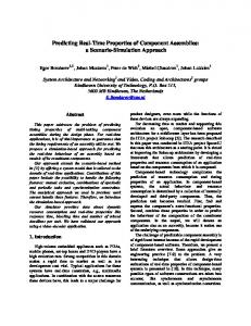
The analysis period has been selected to cover every Wednesday over the period 2 January 1990 - 30 June 1998, based on the yield-curve estimated on the basis of a variant of the doubledecay model from Beaglehole and Tenney (1991). In addition, it has been arbitrarily chosen to re-estimate the model every single Wednesday throughout the period, using an estimation length of 360 days, or to put it more accurately the estimated yield-curves during the last 360 preceding days. Furthermore we have used the following vector of maturity dates as our key-maturity dates: [0.083,0.25,0.5,1,2,3,4,5,7.5,10,12.5,15] - that is P = 12. In connection with the estimation of the model defined in formula 18, it turns out that 4-factors largely explain the entire variation in the term structure of interest rates, where in some periods a 5-factor can be observed, but this 5-factor can be disregarded for all practical purposes. These 4-factors can be called a Level factor, a Slope factor, a Curvature factor and an “residual” factor. These factors each explain about 72.4%, 24.5%, 1.6% and 1.2%, respectively, of the variation in the term structure of interest rates. This result is very similar to Dahl (1989) using Danish data, Litterman and Scheinkmann (1988) and Garbade (1986) using American data, and Caverhill and Strickland (1992) using English data, which conclude that empirically 3 factors exist that describe the dynamics of the term structure of interest rates. However, at this point it should be stressed that Dahl has a somewhat different distribution of the explanatory degree from mine, considering that his factor 1 explains as much as 86% of the variation. An explanation could be that firstly his calculations have been made based on the term structure in 1987 and 1988, and secondly that he uses the Cox, Ingersoll and Ross (1985) model as the basic term structure, which is not as flexible in the context of term structure shapes as the model we have been using for estimating the term structure of interest rates. Figure 1 below show the estimated factor loadings before the varimax rotation and figure 2 show the factor loadings after we have performed the varimax rotation:

11

Empirical Yield-Curve Dynamics, Scenario Símulation and VaR Estimated Faktor Loadings - Original (period 2. January - 30. June 1998) 1.2

Standard Deviation

1 0.8 0.6 0.4 0.2 0 -0.2 -0.4 -0.6 -0.8 0.083 0.25

0.5

1

2

3

4

5

7.5

10

12.5

15

Maturity Faktor Loading 1

Faktor Loading 2

Faktor Loading 3

Faktor Loading 4

Figure 1 E stim ated Faktor Loading s - after V arim ax R otation (pe riod 2. Ja nua ry - 30. June 1998)

Standard Deviation

1 .2 1 0 .8 0 .6 0 .4 0 .2 0 -0 .2 -0 .4 -0 .6 0.08 3 0.25

0.5

1

2

3

4

5

7.5

10

12 .5

M aturity Faktor Loading 1

Faktor Loading 2

Fkator Loading 3

Figure 2

12

Faktor Loading 4

15

Empirical Yield-Curve Dynamics, Scenario Símulation and VaR In figure 3 below we have shown the degree of explanation for each of the factors12:

Degree of Explanation (period 2. January - 30. June 1998) 1.2

Degree of Explanation

1 0.8 0.6 0.4 0.2 0 0.0833

0.25

0.5

1

2

3

4

5

7.5

10

12.5

15

Maturity Faktor 1

Faktor 2

Faktor 3

Faktor 4

Figure 3 Even though these results are not completely independent of the period over which we select to estimate the factor loadings - the factor loadings are very robust as the patterns reported here appear in all cases. The factor loadings are both very robust in connection with the length of the estimation period13, the model used for estimating the yield-curve14 and if we for example had used forward rates or bond returns instead of spot yields.

6.

Measuring of Risk in a multi-factor shift function model

The shift function in this 4-factor term structure model can now be formulated as follows: (21)

12

From now on when we use the phrase factor loading we refer to the factor loadings that are obtained after the varimax rotation. 13

The data period has to be fairly long however in order to have enough degree of freedom to estimate a reasonable covariance matrix. Our experience indicates that at least 1.5 years of data should be used. 14

It is worth pointing out that some problems can be encountered if the estimation procedure is too smooth - which for example would be the case for boot-strapping like estimation procedures.

13

Empirical Yield-Curve Dynamics, Scenario Símulation and VaR where vm, for m = {1,2,3,4} is the vector of factor loadings and dwm is the vector of factor scores. In this connection, the vector sensitivities can be formulated as follows for the coupon bond Pk(t,T): (22)

where this can be regarded as the factor duration. The factor convexity has the following form:

(23)

These two equations deserve a few comments. To fully understand these relations we first note that if we disregard vm, for each m, then the equations degenerate into the portion of returns of the bond which result from a unit change (a standard deviation)15 in the whole yield-curve. The factor model on the other hand tells us that a unit change to the factor does not change the yield-curve by one percent - but by vm percent. From this we can deduce that in order to find the total impact on bond returns from a factor change, we need to scale by a weight that is exactly equal to the appropriate factor loading. 6.1

A practical example - risk factors in the 4-factor term structure model compared with the risk factors in the traditional 1-factor duration model

In order to illustrate the difference between the traditional approach in calculating price sensitivities (i.e. S(t,T) = 0.01), and the price sensitivities generated by this 4-factor model the table below shows the risk calculated using modified duration and the factor duration for a wide range of Danish Government bonds.

Duration Interest Rate Sensitivities as at 30 June 1998

Table 1: Sec. Code 990493

Name of Instrument 12% INK S 2001 01

15

Mod. Duration -1,523

Factor 1 -1,363

S(t,T) = 1%.

14

Factor 2 -0,565

Factor 3 0,249

Factor 4 -0,118

Empirical Yield-Curve Dynamics, Scenario Símulation and VaR 990736

10% INK S 1999 99

-1,033

-0,988

-0,262

0,095

-0,104

990744

10% INK S 2004 04

-3,182

-2,174

-2,030

0,767

-0,065

991015

10% INK S 2001. 01

-1,948

-1,697

-0,818

0,374

-0,143

991619

9% INK St.l}n 00

-2,140

-1,873

-0,893

0,418

-0,160

991716

8% INK St.l}n 03

-4,226

-2,681

-2,998

1,137

-0,011

991783

7% INK St.l}n 04

-5,291

-2,778

-4,184

1,312

0,065

991813

7% INK St.l}n 24

-13,092

-1,072

-12,493

-0,824

-0,581

991821

6% INK St.l}n 99

-1,380

-1,290

-0,416

0,173

-0,130

991864

8% INK St.l}n 06

-6,068

-2,743

-5,089

1,370

0,109

991872

8% INK St.l}n 01

-2,970

-2,336

-1,628

0,735

-0,128

991902

7% INK St.l}n 07

-7,053

-2,396

-6,307

1,177

0,095

991910

6% INK St.l}n 02

-3,848

-2,623

-2,563

1,036

-0,050

991929

6% INK Stgb I 99

-0,617

-0,603

-0,109

0,021

-0,049

991937

4% INK Stgb I 00

-1,578

-1,459

-0,512

0,223

-0,146

991945

5% INK St.l}n 05

-5,903

-2,790

-4,900

1,407

0,112

991961

4% INK Stgb I 01

-2,502

-2,131

-1,145

0,539

-0,168

There is no need to make too many comments about this table, apart from the fact that it is obvious that this 4-factor model measure the risk at the relevant segments/parts of the yieldcurve where the risks of each securities are more logically attributable than what is the case for the traditional 1-factor duration model16. 16

For comparison we have for the same securities shown in Appendix B the traditional convexity concept and the factor convexity.

15

Empirical Yield-Curve Dynamics, Scenario Símulation and VaR This ends the first part of the paper - namely determining the number of factors that drive the evolution in the yield-curve using an empirical approach. We will now turn our focus on efficient methods for simulating yield-curves. Why this is of importance can be formulated as follows.

7.

VaR - a Survey

VaR is probably the most important development in risk management over the past years. This methodology has been specially designed to measure and aggregate diverse risky positions across an entire institution using a common conceptual framework. Even though these measures come under difference disguises e.g. Banker Trusts Capital at Risk (CaR), J.P. Morgans Value at Risk (VaR) and Daily Earnings at Risk (DeaR), they are all based on the same foundation. Even though different institutions has come up with their own names the one that seems to be most commonly used is VaR - which we also will employ here. Definition 1: Risk Capital is defined as the maximum possible loss for a given position (or portfolio) within a known confidence interval over a specific time horizon. VaR plays three important roles within a modern financial institution: ! ! !

It allows risky positions to be directly compared and aggregrated It is a measure of the economic or equity capital required to support a given level of risk activities It helps management to make the returns from a diverse risky business directly comparable on a risk adjusted basis

Even though there are some open issues regarding its calculation, VaR is nevertheless a very useful tool for helping management to steer and control diverse risk operation. The problem with VaR is that there are a variety of different ways to implement the definition of Risk Capital (see Definition 1) each having distinct advantages and weaknesses. In order to get a better grasp of the trade-offs implicit in each method - it is important to understand which kind of components Risk Capital is built around. Risk Capital comprises of the following two (2) distincts parts: ! !

The sensitivity of a position’s (portfolio’s) value to changes in market rates The probability distribution of changes in the market rates over a predefined reporting horizon

Given these assumption - VaR is (usually) defined as the maximum loss within the 99% 16

Empirical Yield-Curve Dynamics, Scenario Símulation and VaR confidence interval. In the following table we have listed the 3 most common methods used when calculating VaR together with their advantages and disadvantages: Method

RiskMetricTM

Delta-Gamma Methods17

Simulation Based Methods

Description

Assume that asset returns are normally distributed, implying linear pay-off profiles and normally distributed portfolio returns18:

Assume that asset returns are normally distributed, but pay-off profiles are approximated by local second order terms

Approximate probability distribution for asset returns based on simulated rate movements, either historically or model based

Advantage

Simplicity.

Simplicity. Captures second order effects.

Captures local and nonlocal price movements. Takes into account fat tails, skewness and kurtosis. With Monte Carlo simulation, we have flexibility to select a probability distribution. With historical simulation we do not need to infer a probability distribution.

Disadvantage

Assuming normality of returns ignores fat tails, skewness and kurtosis. Ignores higher order moments in sensitivities. Captures only risks of local movements for linear securities. Does not capture risks of non-local movements.

Assuming normality of returns ignores fat tails, skewness and kurtosis. Does not capture risks of non-local movements.

Computationally expensive - for Monte Carlo simulation. With Monte Carlo simulation then we need to select a probability distribution. With historical simulation then we cannot select a probability distribution.

It is not directly mentioned in this table but in general it is assumed that the expected return is

17

This method is due to Wilson (1994).

α = 2.54 if we wish to calculate VaR at the 99% confidence level, ∆t = unwind period, V = vector of volatilities and C is the correlation matrix. 18

17

Empirical Yield-Curve Dynamics, Scenario Símulation and VaR zero (0), ie:

. This assumption corresponds closely to the notion of market

efficiency and the random wall hypothesis. The issue that has been mostly widely discussed in the literature with respect to VaR is how to derive appropriate volatility estimates? - see for example Alexander (1996). We will not here discuss that issue but will address it in section 7.3. Another very important issue in connection with VaR is how to derive a reliable correlation matrix? The problem with estimating and modelling the correlation matrix can be summarized as follows: ! !

Correlations coefficients are highly unstable and their signs are ambiguous If for example we have 12 interest rates we need to keep track of (model) correlation coefficients

!

We need a long data period in order to have enough degrees of freedom to estimate a reliable correlation matrix. There is however no guarantee that the resulting matrix satisfy the multivariate properties of the data - we might even encounter a correlation matrix that is not positive definit

These observations have inspired research to reduce the dimensionality - where a common suggested method is PCA - like the one we performed in section 4 and 5 in this paper. The nice property in this context is - as mentioned in section 5 - that even though the correlation coefficients are highly unstable the factor loadings are extremely stable19. Recently Barone-Adesi, Bourgoin and Giannopoulos (1997) has suggested an interesting new approach to worst case scenarios. This method is based on historical returns combined with a GARCH approach (actually a AGARCH-model) for forecasting purposes. The procedure does not employ the correlation matrix directly as the correlation is embedded indirectly in the historical simulation procedure - which is a very neat property of their method. For our implementation of a VaR model we will limit ourselves to domestic interest rate data but extending to multiple currencies is of course possible, this will however not be treated in this paper. Our VaR approach is based on the following basic assumptions: !

We will build our VaR approach on top of our empirical yield curve dynamics model from section 4 and 5

19

The Factor ARCH approach of Engle, Ng and Rothschild (1990) is also in this spirit - see Christiansen (1998) on Danish data.

18

Empirical Yield-Curve Dynamics, Scenario Símulation and VaR ! ! !

7.1

We will estimate the volatility structure using the GARCH approach, see section 7.3 Our approach is a simulation based method which follows along the lines of Jamshidian and Zhu (1997) We will impose the restriction that the expected price change in a discount bond is equal to the price change with arises through the combined effect of a shortening of maturity and a movement down the yield-curve. This means that we will assume that the expected yield-curve will be equal to the initial yield-curve

An Empirical Multi-Factor Model

Before continuing it is worth mentioning that we have the following relationship between dWi (the Wiener process) and dwi (the factor scores), for i = [1,2,3,..,P], and P = number of keyrates (maturities) (in our case 12)20: (24)

this equation arises because dWi .N(0,1) and as we have normalized the correlation matrix21 then and therefore dwi .N(0,1). That is the factor scores are assumed to be standardised normal distributed variables. The equal sign in the last equality in formula 24 becomes an approximation sign for P > 3 where 3 is the number of factors. As follows we have limited ourselves to a 3-factor model as we will consider the fourth-factor to be negligible. Furthermore we assume that the approximation error this gives rise to in equation 24 is negligible. Using the results from section 3 we can in abstract form express the dynamic in the yield-curve as follows: (25) where S(t,T) is the shift-function matrix which in our case for all practical purposes can be fixed to have 3 columns. Furthermore we have that σ(t,T) is a vector of volatilities. The reason why we scale the shift-function is because factor loadings are normalized. 20

For these derivations, we note that if we consider the factor loadings before the varimax rotation - then the correlation matrix is given by KKT and KTK = diag(λ) - if K is the factor loading matrix. It should here be stressed that if we consider the factor loadings after varimax rotation then KTK will only be equal to diag(λ) if the vector of eigenvalues are being recalculated from the factor loading matrix after rotation. In the case that we have not normalized the correlation matrix then λ is the vector of eigenvalues for the correlation matrix. This is however only true if we do not perform varimax rotation of the factors. 21

19

Empirical Yield-Curve Dynamics, Scenario Símulation and VaR The drift in formula 25 depends on the expectation hypothesis, which means that the process has been written under the original probability measure - the implication is that the model as it is formulated in formula 25 is not appropriate for pricing purposes. Using formula 24 and because for our purpose it is more convenient (and appropriate) to assume a lognormal process, we can rewrite formula 25 as: (26)

or alternatively expressed in integral form: (27) We have assumed that µ is equal to the initial yield-curve. That is we assume that the expected yield-curve is equal to the actual yield-curve. This is a more intuitive assumption than using forward rates when our motive is to generate yield-curve scenarios for future dates that are to be used as inputs in various valuation models. The model setup is nevertheless arbitrage free as the uncertainty of each key rate is governed by its own market price of risk - which implicitly are determined through the expectation hypothesis. Again we stress that we are here working under the actual probability measure and not under the risk-neutral probability measure. 7.2

Scenario Simulation

In order to simulate yield-curve movements, we can apply the Monte Carlo method to equation 27. If we now assume that we perform N simulations for each of the 3-factors - then the total number of yield curves at a given point in time will be N3. For N = 100 we will therefore have 1,000,000 future yield-curves which is adequate in order to generate a probability distribution of the future yield curves. However this will require a substantial amount of portfolio evaluation. This approach will for that reason not be of practical use, if firstly the portfolio is fairly large and secondly if the portfolio contains a fair number of non-linear instruments of moderate complexity, like for example Bermudan Swaptions, Barrier options and Mortgage-Backed-Bonds. The interesting question is - how can we reduce the computational burden while at the same time having a reasonable specification of the future yield-curves probability distribution? As shown by Jamshidian and Zhu (1997) this is possible. The argumentation is as follows: Let us suppose that x is a random variable with distribution P(x). In a Monte Carlo method, we simulate N possible outcomes for the random variable x - where each simulated x has the same probability.

20

Empirical Yield-Curve Dynamics, Scenario Símulation and VaR However, we have that numbers xi’s, for i = [1,2,...,N], that falls between xl and xu is proportional to the probability . From this it follows that we can select a region (xl, xu] and assign a given probability for all numbers that fall inside this region. If we utilize this procedure, it is possible for example to perform 100 simulations for each factor but we only need to perform the portfolio evaluation at a limited number of states - more precisely at the number of states that equal the number of predefined regions. A good candidate for a probability distribution is the multinomial distribution22. If k + 1 states (ordered from 0 to k) are selected then the probability for a given state i is given by the binomial distribution and can be expressed as: (28)

For this distribution we have that there is a distance of furthermore is the furthest state

between two adjacent states, and

standard deviation away from the center.

We will now assume that we only need to select nine (9) states for factor 1, five (5) states for factor 2 and three (3) states for factor 323. This gives us all in all 9 x 5 x 3 = 135 scenarios in which we have to evaluate our portfolios - which is independent of the number of Monte Carlo simulations. Under this assumption we get the following probabilities for each of the states for the 3-factors:

(29)

As the 3-factors are independent we have that their joint probability is defined by the products of the three marginal probabilities. We have implemented the technique as follows: Given the number of states for each of the 322

See Cox and Rubenstein (1985).

23

In Jamshidian and Zhu (1997) they select 7,5 and 3 - but as they mention (their footnote 7) the determination of the appropriate number of states for each factor is an empirical question. In section 7.2 we will give evidence that support our decision to have 9 x 5 x 3 states.

21

Empirical Yield-Curve Dynamics, Scenario Símulation and VaR factors we calculate the probability of being in that state for each of the states for each of the 3factors. For each of the 3-factors we now derive the cumulative distribution function given the state-probabilities. After that we utilize the inverse of the normal distribution function in order to determine the random numbers which specify each of the regions. The problem is now boiled down to run a Monte Carlo simulation to select random numbers for the standardized normal distribution and then apply it to the appropriate region. 7.3

An Illustrative Example

In order to show how the approach works we have constructed the following example: The portfolio we have selected is the following:

Example Portfolio as at 30 June 1998

Table 2: Sec. Code

Sec. Name

Position

Clean Price

Accrued Interest

Dirty Price

991937,0000

4% INK Stgb I 00

100000

99,61

1,53

101,14

991716,0000

8% INK St.lån 03

250000

114,35

1,07

115,42

991902,0000

7% INK St.lån 07

135000

115,09

4,43

119,52

991953,0000

6% INK St.lån 09

205000

107,99

3,80

111,79

From table 2 it follows that the value of the portfolio as at 30 June 1998 is 780,211.50 kr. To illustrate the technique we have performed 100 simulations for each of the 3 factors, assigned the simulated random numbers to the appropriate state for that factor and calculated the joint probability. We have used this simulation to calculate the distribution of the portfolio for a 30-day horizon using the factor loadings24 shown in figure 2. The volatility structure we have used as at 30 July 1998 has been forecasted using the GARCH approach and is shown below in figure 4:

24

Though disregarding the fourth factor.

22


Volatility Forecast - GARCH 40

Volatility p.a.

35 30 25 20 15 10 5 0 0.0833

0.25

0.5

1

2

3

4

5

7.5

10

12.5

15

Maturity Volatility - GARCH

Figure 4 For the interested reader we have in Appendix C briefly discussed the idea behind GARCH and also explained how we have constructed the forecasted volatility structure. Before we are able to determine the distribution of the value of the portfolio we need to address one more issue - namely the building of a yield-curve given the price of zero-coupon bonds at the following fixed maturity dates: [0.083,0.25,0.5,1,2,3,4,5,7.5,10,12.5,15]. For that purpose we are using the maximum smoothness approach of Adams and Deventer (1994), see Appendix D for an elaboration. In figure 5 below we have shown the distribution of the portfolio value at 30 July 1998 using the scenario simulation approach described in section 7.2 and compared it to the normal distribution which has a first-and second order moment equal to the empirical distribution:

23


Probability

Simulated Horizon Portfolio Distribution 1 0.9 0.8 0.7 0.6 0.5 0.4 0.3 0.2 0.1 0

14 12 10 8 6 4 2 0 761040 765907 770774 775640 780507 785374 790240 795107 799974 804841 0 763474 768340 773207 778074 782940 787807 792674 797540 802407

Portfolio Value Intervals Calculated Frequency

Theoretical Frequency

Calculated Probability

Theoretical Probability

Figure 5 We have also tested the hypothesis that the portfolio distribution is normally distributed25 and can report the following:

Goodness Of Fit-Test

Table 2: χ2

8,47

Degrees of Freedom

20

Level of Significance

0,9883

As a comparison in figure 6 we have shown the portfolio distribution using Monte Carlo simulation with the number of future yield-curves equal to 503 - 125.000 simulations (that is 50 simulations for each factor)26:

25

It should be noted here that as interest rates are lognormal and for that reason log-prices are lognormally distributed this mean that we cannot derive the probability distribution of bond-prices. This indicates that we would expect the portfolio value not to be normally distributed. We however fail to reject that hypothesis, even though we observe fatter tails. 26

We have for practical reasons restricted ourselves to 50 simulation per factor instead of 100 - but 125,000 future yield-curves is sufficient to generate a probability distribution. It should be stressed here that a normal distribution assumption is clearly rejected for the Monte Carlo simulated portfolio value.

24


Probability

Monte Carlo Simulated Horizon Portfolio Distribution 1 0.9 0.8 0.7 0.6 0.5 0.4 0.3 0.2 0.1 0

18000 16000 14000 12000 10000 8000 6000 4000 2000 0 760751 765091 769431 773771 778111 782451 786791 791131 795471 799811 0 762921 767261 771601 775941 780281 784621 788961 793301 797641

Portfolio Value Intervals Calculated Frequency

Theoretical Frequency

Calculated Probability

Theoretical Probability

Figure 6 To further compare the scenario simulation procedure with the full Monte Carlo simulation technique we have in table 3 below shown various statistics: Table 3:

Various Statistics for the Simulated Portfolio Value Scenario Simulated Portfolio Value (9 x 5 x 3)

Monte Carlo Simulated Portfolio Value (125000)

783831,94

782992,94

10654,32

6473,06

Skewness

-0,08

-0,23

Kurtosis

2,43

2,61

Maximum

807273,87

801980,81

Minimum

758606,89

758581,34

Mean - Expected Portfolio Value Standard Deviation

To select to simulate 9,5, and 3 states for the 3-factors is as mentioned a subjective decision. In order to analyse the significance of this decision we have also performed the portfolio valuation for the following combinations:

25

Empirical Yield-Curve Dynamics, Scenario Símulation and VaR 3-Factors - 7 x 5 x 3 2-Factors - 9 x 5 2-Factors - 7 x 5

! ! !

For these different scenario simulation procedures we can report the following:

Various Statistics for the Scenario Simulated Portfolio Value

Table 4:

Scenario Simulated Portfolio Value (7 x 5 x 3)27

Scenario Simulated Portfolio Value (9 x 5)

Scenario Simulated Portfolio Value (7 x 5)

783861,66

783833,96

783863,68

10229,01

10696,37

10288,70

Skewness

-0,07

-0,08

-0,07

Kurtosis

2,34

2,42

2,33

Maximum

805431,49

806281,25

804428,31

Minimum

760895,35

759812,80

762088,92

Mean - Expected Portfolio Value Standard Deviation

From the results in table 3 and table 4 we conclude the following: The scenario simulation procedure generates a mean that is very close to the mean derived from the Monte Carlo simulation - this is the case for all the 4 scenario simulations ! The standard deviation in the scenario simulations is in all cases higher than the standard deviation obtained in the Monte Carlo simulation. The reason for this is because in the scenario simulations we give relatively more weight to factor 1 and because the volatility structure is downward sloping. In the Monte Carlo simulation each factor is given equal weights28 ! In general we have relatively more observations in the tails for the scenario simulation than for the Monte Carlo simulation (this can also be observed in figure 5 and figure 6) ! We also observe that the maximum value obtained in the scenario simulation is higher than the one we get from the Monte Carlo simulation It also seems to be the case that for all practical purposes we can disregard factor 3. However !

27

This is the combination suggested by Jamshidian and Zhu (1997).

28

We could of course also have chosen to weight factor 1 relatively more in the Monte Carlo simulation. If we had done that the standard deviation obtained from the Monte Carlo method would have been closer to the standard deviation derived from the scenario simulation procedure.

26

Empirical Yield-Curve Dynamics, Scenario Símulation and VaR this observation might be explained by the fact that the portfolio we have been using in our example is a very simple portfolio as it only consist of securities with a nearly linear price-yield relationship29. Knowing the probability distribution makes it straightforward to calculate VaR. This is done below in table 5 where as comparison we have also shown VaR calculated in a parametric fashion using the RiskMetricTM-approach. Table 5: Calculated

30-day VaR (Percentage of primo Portfolio Value)30 95%-Confidence Level

97.5%Confidence Level

99%-Confidence Level

Monte Carlo Simulated VaR (125000)

1,3295

1,5328

1,7770

Scenario Simulated VaR (9 x 5 x 3)

1,8748

2,3952

2,7852

Scenario Simulated VaR (7 x 5 x 3)

1,7782

2,2087

2,5387

Scenario Simulated VaR (9 x 5)

1,9480

2,6014

2,6949

Scenario Simulated VaR (7 x 5)

1,9601

2,3937

2,4256

Parametric VaR31 (RiskMetricTM Methodology)

1,7910

2,0470

2,3570

As can be seen in table 5 it actually might not be that important to include factor 3. As a matter of fact there is evidence that support that it is more appropriate to select 9 x 5 states than 7 x 5 x 3 states. From this we deduce that it is probably more important to have more states for factor 1 than including factor 3. For this analysis we will though assume that 9 x 5 x 3 states are 29

By nearly we mean that the convexity is approximately negligible for these securities.

30

That means that the figures in the table can be thought of as some kind of duration measures.

31

We have calculated the Parametric VaR by using equation 22 though scaled by respectively 1.96σP(t,T)∆t0.5, 2.24σP(t,T)∆t0.5, 2.58σP(t,T)∆t0.5, for ∆t = 30 days (the unwind period). We find the bond-price volatility using the following formula: . This technique is in principle identical to the RiskMetricTM-approach. The difference is that in RiskMetricTM the adjustment parameter is made to the traditional 1-factor duration measure - more precisely the adjustment is given by

- where C is the

correlation matrix, V is a vector of bond price volatilities and α is defined as respectively 1.96, 2.24 and 2.58.

27

Empirical Yield-Curve Dynamics, Scenario Símulation and VaR neccesary and sufficient. It is important to point out a few things with repect to the VaR figures obtained from the Monte Carlo procedure. For example at the 99% confidence interval we still have 1250 observation left in the tails, which mean that we have to go to the 99.99% fractile in order to get an observation which lies close to the minimum - at the minimum it is worth mentioning that we have a value of 2.7724. This is actually a general feature of Monte Carlo simulation and VaR - a confidence level which usually is considered to be appropriate might fail to produce a reasonable VaR number - because of the close distance between observations. This is a problem with Monte Carlo simulation and VaR that has been neglected in the literature, where Monte Carlo simulation - if no other alternative is available - is considered the solution32. However, the popularity of crude Monte Carlo simulation might be exaggerated, the reason being that there is no control over the extreme values in Monte Carlo simulation - which is where our interest lies in the calculation of VaR. Of course it could be argued that a stress analysis would have revealed an appropriate VaR number - which is true. The scenario analysis will on the other hand - if the states are properly selected - always give an appropriate VaR number. By properly selected I mean that it is important to have states which also put emphasis on extreme observations - which is exactly the case for the 9 x 5 x 3 selection. Table 5 actually supports our decision to select 9 x 5 x 3 states for the 3-factors33. This is different from what Jamshidian and Zhu advocate (remember they suggest 7 x 5 x 3). However in an environment with a falling volatility structure, with a 1 factor that dominates over the other factors and where the movement in the short end of the yield-curve is governed by the 1. factor - it seems more appropriate to put some additional weight on this factor. The analysis performed in this section gives rise to the following conclusion: ! !

!

The scenario simulation procedure is computationally very superior to the Monte Carlo simulation procedure In the scenario simulation procedure there is much better control over the extreme values than in the Monte Carlo simulation, which is an attractive feature from a risk-management point of view. This means that it is more straightforward to select a confidence level and get results which are correct/reliable If we believe that the 3 factors we found in section 5 and their ranking are of a kind that is generally observed, then the scenario simulation procedure is much better than the Monte Carlo simulation procedure in taking into account the relative importance of each of the factors. This is of special importance if we observe a falling volatility structure, which usually happens

32

Even if another method is available (like for example the parametric approach for “linear” securities) the Monte Carlo procedure is probably the most popular method in the literature for calculating VaR. 33

Though the selection of 9 x 5 states would be a good alternative.

28


!

7.4

to be the case. The importancy is examplified by the difference in standard deviation in table 3 There is also evidence that it is appropriate to select 9 x 5 x 3 states (or maybe 9 x 5 states) when using the scenario simulation approach

Scenario Simulation for Non-linear Portfolios

Even though the parametric VaR approach does not perform too badly (at least for the 99%confidence interval), the normal distribution assumption which underlies the calculation clearly underestimates the tails of the distribution. Futhermore the scenario simulation procedure is so fast for simple (nearly) linear instruments that it rivals the parametric approach. Actually the scenario simulation takes less than 3 seconds34 all in all, where this includes: ! ! ! ! ! ! !

Simulating 3 x 100 random numbers Assigning the random numbers to the proper states Calculating the probability for realising a particular yield curve Calculating the 135 yield curves for the 12 maturities Estimating 135 yield curves using the maximum smoothness approach of Adams and Deventer (1994) Calculating the price distribution of each of the 4-bonds in the portfolio Calculating VaR for a given confidence interval

The calculation of the price distribution of the 4 bonds takes approximately 2 seconds. From this we conclude that there is no reason why we should be satisfied with a single number from a risk-management point of view - when we can construct a probability distribution with fatter tails than the normal distribution and with very little effort from a computational perspective. Of course scenario simulation is even more important for non-linear securities. We will for that reason turn our attention to some interesting non-linear securities - namely Danish MortgageBacked-Bonds35. Here we will not focus on a portfolio but instead select a few different MBBs and then use the scenario simulation procedure to calculate the probability distribution for these securities. However, expanding to a portfolio approach is straightforward as the probability distribution of a portfolio is just defined as the value-weighted sum of the probability distributions for each of the securities in the portfolio. For the purpose of the following discussion we assume that a pricing model is available. I will however here mention a few of the ingredients that are an integrated part of a pricing model for 34

We ran the program on a 300 Pentium II.

35

For a good introduction to Danish Mortgage-Backed-Bonds, see Karner, Kelstrup and Schelde (1998) and Kelstrup, Madsen and Rom-Poulsen (1999).

29

Empirical Yield-Curve Dynamics, Scenario Símulation and VaR Danish MBBs (and for that matter American MBBs): ! ! !

! !

A yield-curve estimated using government securities A prepayment model for the behaviour of the debtors - we are here using the Madsen (1998) model A model for the credit-spread between the mortgage market and the government market - we are here using the framework described in Madsen (1997) A model for the volatility structure - we are here using the GARCH framework A pricing model that uses the first four ingredients to calculate the price - we are here using the Black and Karisinski (1991) model, though calibrated using the trinomial approach of Hull and White (1994)

As far as we know VaR for Danish MBBs has only been considered by Jacobsen (1996), his method is however completely different than the methodology we employ in this paper. Let me for that reason briefly mention a few stylized facts about Jacobsens approach: The main idea in Jacobsen is to construct a delta equivalent hedge portfolio of zero-coupon bonds - that is a 1 order approximation. For that purpose he selects 17 key-rates36 and using the triangular method of Ho (1992) it is possibly to construct 17 different shifts to the initial yieldcurve - where these shifts by definition are constructed in such a manner that the sum of the shifts equals an additive shift to the yield-curve. This delta equivalent hedge portfolio is now being used to calculate VaR measures using the parametric approach suggested in RiskMetricTM for linear securities - that is the delta equivalent cash-flow (DECF) is being treated as a straight bond. This approach is very simple and the computational burden is acceptable - “just” 17 price calculations - but there are some undesirable features in the methodology: !

!

Firstly, the DECF is not constant, it depends on all the information that is related to the pricing of MBBs (this is also pointed out by Jacobsen). This means that it is probably only useful for calculating VaR over short periods and this even in a situation where we have made a convexity adjustment as suggested by Wilson (1994) - the Delta-Gamma approach Secondly, it does not produce a probability distribution - which especially for non-linear securities is of importance. Offcourse we can construct a probability distribution using the DECF approach - but because the DECF is not constant - this probability distribution will not be of any interest/use

It could of course be argued that in the scenario simulation procedure advocated here we need

36

The reason being that this is the number of maturities that RiskMetricTM operates with.

30

Empirical Yield-Curve Dynamics, Scenario Símulation and VaR to perform 135 price calculations in order to derive the probability distribution - which is not feasible37 for large portfolios of MBBs. Of course we might also be able to limit ourselves to 9 x 5 states as in the last example without losing to much information - but for now we will assume that we need to include factor 3. Let us now turn our attention to the problem at hand - namely calculating VaR for Danish MBB. In table 6 below we have listed the 4 different MBBs, we have chosen for our analysis.

A Selection of Danish MBB (30. June 1998)

Table 6: Sec. Code

Sec. Name

Clean Price

Accrued Interest

Dirty Price

926256,0000

5% 23D s. 29

92,55

0,03

92,58

925799,0000

6% 23D s. 29

97,75

0,03

97,78

925802,0000

7% 23D s. 29

101,70

0,04

101,74

925810,0000

8% 23D s. 29

102,15

0,04

102,19

In order to illustrate the asymmetric behaviour for these securities we have in figure 7 below shown their price sensitivities against parallel shift in the yield-curve as at 30 June 1998.

37

I will not directly address this issue here, instead I will analyse how our methodology behaves for Danish MBBs. However I will state here - without proof - that this methodology is feasible for large portfolios of MBBs. How exactly we do that lies however outside the boundary of this paper, for elaboration see Madsen (1999).

31

Empirical Yield-Curve Dynamics, Scenario Símulation and VaR Price Sensitivities (pr. 30. June 1998)

10.0

20.0 15.0

5.0 Percentage PriceSensitivity

10.0 0.0

5.0

-5.0

0.0 -5.0

-10.0

-10.0 -15.0

-15.0

-20.0

-20.0 -1.50 -1.25 -1.00 -0.75 -0.50 -0.25 0.00 0.25 0.50

0.75 1.00

1.25 1.50

Additive Shift in the Yie ld-Curve 925799 6% 23D s. 29

925802 7% 23D s. 29

925810 8% 23D s. 29

926256 5% 23D s. 29 - (right axis)

Figure 7 As seen from this figure we have selected 4 different MBBs with very different price sensitivities: ! !

!

!

The 5% 2029 behaves approximately like a straight bond (the bond has positive convexity) The 6% 2029 is assymetric - it behaves like a straight bond if rates goes up but is hit by the rise in prepayment if rates fall, however there is still some potential in a falling interest rate enviroment (the bond has high negative convexity) The 7% 2029 is assymetric - is behaves like a straight bond when rates go up but its upside potential in a falling yield-curve environment is limited (the bond has high negative convexity) The 8% 2029 is close to being independent of the changes in interest rates some movement is however noted for a large rise in interest rates (the bond has close to zero in convexity)

These conclusions depends of course on two things. Firstly the range of interest rates changes, and secondly that we only consider additive shifts in the initial yield-curve. However, figure 7 still gives a very good picture of the asymmetric property of Danish MBBs. Using the scenario simulation procedure we will now derive the probability distribution of these 4 MBBs at 30 July 1998 - where we are using the same assumptions as the one from section 7.3. The results are shown below in figure 8: 32


0.4

15

0.3

10

0.2

5

0.1

0

0

6.

5.

5.

4.

3.

2.

1.

0.

0.

-0

-1

-2

-3

Probability

20

72

0.5

89

25

06

0.6

23

30

39

0.7

56

35

73

0.8

90

40

07

0.9

.7 6

45

.5 9

1

.4 3

50

.2 6

Frequency

Comparison of Probability Distributions

Price Sensitivities Frequency 5% 2029

Frequency 6% 2029

Frequency 7% 2029

Frequency 8% 2029

Probability 5% 2029

Probability 6% 2029

Probability 7% 2029

Probability 8% 2029

Figure 8 The price sensitivities - or HPR (holding period return) - is defined as:

, for i =

[1,2,3,...,135]. In order to get a better picture of the difference between the distribution of each of the bonds in table 7 below we have shown various statistics. In this table we have also calculated VaR for each of the bonds at the 95%, 97.5% and 99% confidence level - which are easily derived from the probability distributions. Table 7:

Statistics for the Scenario Simulated Distributions 5% 23D s. 2029

6% 23D s. 2029

7% 23D s. 2029

8% 23D s. 2029

Mean - Expected Return

1,66

1,40

0,14

-0,36

Standard Deviation

2,94

2,20

0,80

0,47

33

Empirical Yield-Curve Dynamics, Scenario Símulation and VaR Skewness

-0,08

-0,19

-0,40

0,21

Kurtosis

1,90

2,05

2,80

2,74

Maximum

6,72

5,29

1,50

0,80

Minimum

-3,67

-3,16

-2,17

-1,41

VaR - 95% Confidence Level

3,05

2,46

1,35

1,08

VaR - 97.5% Confidence Level

3,38

2,92

1,83

1,16

VaR - 99% Confidence Level

3,63

3,14

2,07

1,22

The VaR number reported here and in table 5 must of course be evaluated which will be done in section 7.5. 7.5

Test of the VaR Scenario Simulation Procedure

In order to evaluate the VaR figures we have performed the following tests: !

!

For the 4 MBBs in table 6 and 2 of the government Bonds in table 2 we have calculated VaR - more precisely the 30-day (monthly) VaR. This we have done at the following dates: 30 June 1998, 30 July 1998 and 31 August 1998 - that is at the end of every month. We will in this connection use the 99% confidence interval as our measure of VaR For each of the 6 bonds we have calculated the monthly return38 over the period 30 June 1998 - 30 September 1998

The period we have selected is not particular long but one important aspects of this period is the currency crises in mid september. It is especially these kind of extraordinare market events we want our VaR model to capture. In table 8 below we have listed the VaR at the 99% confidence interval for all the 6 bonds in question:

38

The monthly return in calculated as follows: the three month period is being devided into three (3) onemonth periods. The monthly return is then calculated as the monthly return since the end of the last month.

34

Empirical Yield-Curve Dynamics, Scenario Símulation and VaR Monthly VaR 99% Confidence Interval

Table 8: Sec. Code

Sec. Name

30. June 1998

30. July 1998

31. August 1998

991716

8% INK St.lån 03

2,55

2,59

2,68

991953

6% INK St.lån 09

3,46

3,45

3,41

926256

5% 23D s. 29

3,63

3,71

7,89

925799

6% 23D s. 29

3,14

3,20

6,55

925802

7% 23D s. 29

2,07

2,39

3,79

925810

8% 23D s. 29

1,22

1,60

0,60

We have in figure 9 below shown the default-free yield-curves at 30. June 1998, 30. July 1998 and 31. August 1998 and as a comparison we have also included the credit-adjusted yieldcurves for the same 3-dates:

Comparison of Credit-Adjusted Yield-Curves and Default-Free Yield-Curves

7.5 7

Interest Rate

6.5 6 5.5 5 4.5 4 3.5 28.8

27.3

25.8

24.3

22.8

21.3

19.8

18.3

16.8

15.3

13.8

12.3

10.8

9.25

7.75

6.25

4.75

3.25

1.75

0.25

3

M aturity Credit-Adjusted - 30. June 1998

Credit-A djusted - 30. July 1998

Credit-Adjusted - 31. August 1998

Government - 30. June 1998

Government - 30. July 1998

Government - 31. August 1998

Figure 9 In Appendix E we have in 3-dimensional graphic visualized the 3-pairs of simulated creditadjusted yield-curves. We have not included the simulated default-free yield-curves as the pattern closely resembles the one reported in the graphs for the credit-adjusted yield-curves though the levels are different.

35

Empirical Yield-Curve Dynamics, Scenario Símulation and VaR The drastic change in VaR for the 4 MBB’s for the 31. August 1998 compared to the two previous month can be derived from the following stylized facts about yield-curve changes and price sensitivities of MBBs: !

!

!

MBBs is sensitive to changes in the short end of the term structure - that is MBBs is especially sensitive to changes in factor 1. This is true regardless of the MBBs sensitivity against parrallel shift in the yield-curve. This means that even though the 8% 2029 looks like it is in-sensitive to changes in the yieldcurve this is not the case. More precisely we have that the price of MBBs is negatively correlated to changes in the short end of the yield-curve MBBs are sensitive to changes in the long end of the curve (factor 2). However in this case we have no clear pattern, but we can conclude the following: ! For MBBs with approximately no sensitivity against parallel shift in the yield-curve - we have that the price is positively correlated to changes in the long end of the yield-curve ! For MBBs with has sensitivity against parallel shift in the yield-curve - at least in a rising yield-curve enviroment, we have that the price is negatively correlated to changes in the long end of the yield-curve In general we do not observe much sensitivity for MBBs against changes in the curvature of the yield-curve - that is factor 3 does not seem to be that important for MBBs

These conclusion is supported by the graph in figure 10. In figure 10 we have shown the percentage price changes for the 4 MBBs as a function of the 9 x 5 x 3 simulated yield-curves where we arbitrary has selected the simulated yield-curves pr. 30. July 1998.

36

Empirical Yield-Curve Dynamics, Scenario Símulation and VaR Price Changes as a function of the Scenario Simulated Yield-Curves 8

Percentage price change

6 4 2 0 -2 -4

133

127

121

115

109

103

97

91

85

79

73

67

61

55

49

43

37

31

25

19

7

13

1

-6

Simulations number 5% 2029

6% 2029

7% 2029

8% 2029

Figure 10 This figure is to be understood as follows: ! ! !

The figure is split into 3-parts, where this represents the 3 states selected for factor 3 - the curvature factor Each of these 3-parts is then further divided into 5 states - representing the states selected for factor 2 - the long factor These 5 states are then further divided into 9 states - representing the states selected for factor 1 - the short factor

In the following three (3) figures we have shown VaR and the monthly return for the 3-month period covering 30. June 1998 - 30. September 1998 for 6% 2029, 7% 2029 and 8% 202939:

39

The same charts for the three (3) last security codes are shown in Appendix F.

37

19 98 07 01 19 98 07 07 19 98 07 13 19 98 07 17 19 98 07 23 19 98 07 29 19 98 08 04 19 98 08 10 19 98 08 14 19 98 08 20 19 98 08 26 19 98 09 01 19 98 09 07 19 98 09 11 19 98 09 17 19 98 09 23 19 98 09 29 80 19 70 98 1 0 19 706 98 0 19 70 98 9 0 19 714 98 0 19 717 98 0 19 72 98 2 0 19 727 98 0 19 73 98 0 0 19 804 98 0 19 807 98 0 19 81 98 2 0 19 817 98 0 19 82 98 0 0 19 825 98 0 19 82 98 8 0 19 902 98 0 19 907 98 0 19 91 98 0 0 19 915 98 0 19 91 98 8 0 19 923 98 09 28

19 9

Empirical Yield-Curve Dynamics, Scenario Símulation and VaR M o n th ly retu rn an d V aR 6% 23D s. 29

3.00

2.00

1.00

0.00

-1.00

-2.00

-3.00

-4.00

-5.00

-6.00

-7.00

Monthly retur n

1.00

Monthly return Monthly V aR

Figure 11

Monthly return and VaR 7% 23D s. 29

0.50

-0.50 0.00

-1.00

-1.50

-2.00

-2.50

-3.00

-3.50

-4.00

-4.50

Monthly VaR

Figure 12

38


1.00

Monthly return and VaR 8% 23D s. 29

0.50 0.00 -0.50 -1.00 -1.50

19 9

19 9

80 70 1 80 70 19 7 98 07 13 19 98 07 17 19 98 07 23 19 98 07 29 19 98 08 04 19 98 08 10 19 98 08 14 19 98 08 20 19 98 08 26 19 98 09 01 19 98 09 07 19 98 09 11 19 98 09 17 19 98 09 23 19 98 09 29

-2.00

Monthly return

Monthly V aR

Figure 13 Optimal we would like the VaR number to represent a lower barrier where the monthly return cannot cross. This is of course to much to hope for - we can only expect that 99% of the monthly returns lies above the VaR barrier. From figure 11-13 and the chart in Appendix F the VaR model appears to be fairly robust - as it generally manages to capture the extreme events that occured during the currency crisis in september. Though there is one observation for the 8% 2029 the model fail to capture. This observation (outlier for the 8% 2029) would however have been captured if we had been running not monthy VaR but weekly VaR numbers. Of course more empirical investigations are required of the ability of the model to forecast a lower barrier for returns (price changes). The findings in this paper are though promising. From the analysis in this section we will conclude the following with respect to the scenario simulation procedure advocated here: ! !

!

The scenario simulation procedure is a computational effective alternative to Monte Carlo simulation The scenario simulation procedure is capable of producing very good approximations of the probability distributions with a limited number of states There is much better control over the extreme values in the scenario simulation than in Monte Carlo simulation 39

Empirical Yield-Curve Dynamics, Scenario Símulation and VaR !

!

!

The scenario simulation procedure is more efficient than the parametric approach for “linear” securities and it rivals the parametric approach for “linear” securities because of the speed of calculation We suggested using 9 x 5 x 3 states for the scenario simulation. However in some cases (maybe in most cases) we would only need to consider 9 x 5 states. Because we “only” need to perform 135 (maybe just 45) re-evaluations of the portfolio the scenario simulation procedure is feasible for large portfolios consisting of highly complex non-linear securities One last important feature is that the scenario simulation procedure uses the fact that changes in the yield-curve is empirically driven by 3-factors: A Short Factor, a Long Factor (Slope Factor) and a Curvature Factor

Apart from the additional work that is needed on empirical testing the VaR model there is still work to do in connection with the inputs that are required for the scenario simulation procedure, the following things need to be considered: !

!

!

8.

How to forecast the volatility? " In this paper we argued that GARCH is a logical method to utilize but other procedures like for example stochastic volatility models also need to be considered What is the proper horizon for calculating VaR? " In this paper we only considered 30-days VaR (monthly VaR) - but we believe that it is appropriate to also have a 7-days VaR (weekly VaR) How to select the expected yield-curve at a given time-horizon? " In this paper we suggested using the initial yield-curve as the expected yield-curve. Another alternative would of course have been to use the implied forward-rate curve.

Conclusion

The first result in this paper was the construction of a general model for the variation in the term structure of interest rates - that is we defined a model for the shift function. In this connection we showed - using the Heath, Jarrow and Morton (1991) framework - that the shift function could be understood as a volatility structure - more precisely the spot rate volatility structure. The class of shift functions considered in this paper was of the linear type, with independence between the individual factors; the model was therefore comparable to the Ross (1976) APT model. Using PCA we showed that it took a 4-factor model (which, in principle, could very well be considered a 3-factor model due to the limited effect of factor four (4)) to explain the variation in the term structure of interest rates over the period from the beginning of 1990 to mid-1998. 40

Empirical Yield-Curve Dynamics, Scenario Símulation and VaR These 4 factors can be called a Level factor, a Slope factor, a Curvature factor and an “residual” factor. These factors each explain about 72.4%, 24.5%, 1.6% and 1.2%, respectively, of the variation in the term structure of interest rates. This result is in line which what normally is reported in the literature, see for example Litterman and Scheinkman (1988). Because of the relationship between the volatility structure in the Heath, Jarrow and Morton framework and the shift function implied from our empirical analysis of the evolution in the yield-curve we concluded that PCA could be used to determine the volatility structure in the Heath, Jarrow and Morton framework - a non-parametric approach. It was moreover argued that calculating price sensitivities in this multi-factor model was relevant, as a great degree of stability in the estimated factor loadings could be observed. In the last part of the paper we turned our attention to VaR models. Our approach to the calculation of VaR is a scenario simulation based methodology with relies on the framework of Jamshidian and Zhu (1997). This scenario simulation procedure builds on the factor loadings derived from a PCA of the same kind we used in our analysis of the empirical dynamics in the yield-curve. The general idea behind the scenario simulation procedure is to limit the number of portfolio evaluations by using the factor loadings derived in the first part of paper and then specify particular intervals for the Monte Carlo simulated random numbers and assign appropriate probabilities to these intervals (states). From our analyses of both straight bonds and Danish MBBs using the scenario simulation procedure we conclude the following: ! !

! !

!

!

The scenario simulation procedure is a computational effective alternative to Monte Carlo simulation The scenario simulation procedure is capable of producing very good approximations of the probability distributions with a limited number of states There is much better control over the extreme values in the scenario simulation than in Monte Carlo simulation The scenario simulation procedure is more efficient than the parametric approach for “linear” securities and it rivals the parametric approach for “linear” securities because of the speed of calculation We suggested using 9 x 5 x 3 states for the scenario simulation. However in some cases (maybe in most cases) we would only need to consider 9 x 5 states. Because we “only” need to perform 135 (maybe just 45) re-evaluations of the portfolio the scenario simulation procedure is feasible for large portfolios consisting of highly complex non-linear securities One last important feature is that the scenario simulation procedure uses the fact that changes in the yield-curve is empirically driven by 3-factors: A Short Factor, a Long Factor (Slope Factor) and a Curvature Factor 41

Empirical Yield-Curve Dynamics, Scenario Símulation and VaR We also tested the VaR model for 6 bonds (2 government bonds and 4 MBBs) for the 3. quarter of 1998 and found the model to be fairly robust. In all the cases excepts one (1) the VaR model managed to capture the extreme movements influenced by the currency crisis in september 1998. More work is of course necessary - both with respect to backtesting the model and with respect to the determination of the input to the scenario simulation procedure. In connection with the inputs to the scenario simulation method we especially need to address the following: ! ! !

How to forecast the volatility? " In this paper we argued that GARCH is a logical method to utilize What is the proper horizon for calculating VaR? " In this paper we only considered 30-days VaR (monthly VaR) How to select the expected yield-curve at a given time-horizon? " In this paper we suggested using the initial yield-curve as the expected yield-curve

Literature Adams and Deventer (1994) “Fitting Yield Curves and Forward Rates with Maximum Smoothness”, Journal of Fixed Income vol. 4, no. 1, page 52-62 Alexander (1996) (editor) “Risk Management and Analysis”, John Wiley and Sons 1996 Amin and Morton (1993) "Implied Volatility Functions in Arbitrage Free Term Structure Models", Working Paper University of Michigan, May 1993 Barrett, Heuson and Gosnell (1992) "Yield Curve Shifts: An Empirical Solution to a Theoretical Dilemma", Working Paper, University of Miami, October 1992 Baron (1989) "Time Variation in the Modes of Fluctuation of the Treasury Yield Curve", Bankers Trust, October 1989 Barone-Adesi, Bourgoin and Giannopoulos (1997) “A Probabilistic Approach to Worst Case Scenarios”, working paper University of Westminster, August 1997

42

Empirical Yield-Curve Dynamics, Scenario Símulation and VaR Beaglehole and Tenney (1991) "General Solutions of some Interest Rate-Contingent Claim Pricing Equations", Journal of Fixed Income 3, pp. 69-83 Berndt, Hall, Hall and Hausman (1974) “Estimation and Inference in Nonlinear Structural Models”, Annals of Economic and Social Management 3/4, page 653-665 Bierwag, Kaufmann and Toevs (1983) "Innovation in Bond Portfolio Management", JAI Press Inc. Bierwag (1987a) "Duration Analysis Managing Interest Rate Risk", Balling Publishing Company 1987 Bierwag (1987b) "Bond Returns, Discrete Stochastic Processes, and Duration", Journal of Financial Research 10, pp. 191-209 Bierwag, Kaufmann and Latta (1987) "Bond Portfolio Immunization: Tests of Maturity, Oneand 2-factor Duration Matching Strategies", Financial Review 22, pp. 203-219 Black and Karasinski (1991) "Bond and Option pricing when short rates are lognormal", Financial Analyst Journal, July-August 1991, page 52-69 Bollerslev (1986) "Generalized Autoregressive Conditional Heteroskedasticity", Journal of Economtrics 31, page 307-327 Boudoukh. Richardson and Whitelaw (1997) “Investigation of a Class of Volatility Estimators”, Journal of Derivatives vol. 4, no. 3, page 63-71 Caverhill and Strickland (1992) "Money Market Term Structure Dynamics and Volatility Expectations", Working Paper, University of Warwick, June 1992 Chambers, Carleton and Waldman (1984) "A New Approach to Estimation of the Term Structure of Interest Rates", Journal of Financial and Quantitative Analysis, Vol. 19, pp. 233252 Chambers and Carleton (1988) "A Generalized Approach to Duration", Research in Finance, Vol. 7, pp. 163-181 Chambers, Carleton and Mcenally (1988) "Immunizing Default-Free Bond Portfolios with a Duration Vector", Journal of Financial and Quantitative Analysis, pp. 89-104 Christiansen (1998) “Value at Risk Using the Factor-ARCH Model”, working paper D 98-6, Department of Finance, The Aarhus School of Business Cox, Ingersoll and Ross (1985) "A Theory of the Term Structure of Interest Rates", Econometrica 53, pp. 363-385 43

Empirical Yield-Curve Dynamics, Scenario Símulation and VaR Cox and Rubinstein (1985) “Options Markets”, Englewood Cliffs: Prentice Hall 1985 Dahl (1989) "Variations in the term structure of interest rates and controlling interest-rate risks" [in Danish], Finans Invest, February 1989 Elton, Gruber and Nabar (1988) "Bond Returns, Immunization and The Return Generating Process", Studies in Banking and Finance 5, pp. 125-154 Engle (1982) "Autoregressive Conditional Heteroskedasticity with Estimates of the Variance of United Kingdom Inflation", Econometrica vol 50, no. 4, page 987-1007 Engle and Ng (1991) “Measuring and Testing the Impact of News on Volatility”, working paper University of California Engle, Ng and Rothschild (1990) “Asset Pricing with a Factor-ARCH covariance structure”, Journal of Econometrics 45, page 213-237 Garbade (1986) "Modes of Fluctuations in Bonds Yields - an Analysis of Principal Components", Bankers Trust, Money Market, June Garbade (1989) "Polynomial Representations of The Yield Curve and its Modes of Fluctuation", Bankers Trust, July 1989 Giannopoulos (1995) “The Theory and Practice of ARCH Models”, working paper University of Westminster, 27 November 1995 Glosten, Jagannathan and Runkle (1991) “Relationship Between the Expected Value and the Volatility of the Nominal Excess Return on Stocks”, working paper Northwestern University Golub and Van Loan (1993) “Matrix Computations”, The John Hopkins University Press, second edition 1993 Greene (1993) "Econometric Analysis", 2nd Edition, Macmillan Publishing Company 1993 Hald (1979) “Updating formulas in Quasi-Newton methods” (in Danish), Department for Numerical Analysis, report no. NI-79-03 Harman (1967) "Modern Factor Analysis", University of Chicago Press, 1966 Harvey, Ruiz and Shepard (1994) “Multivariate Stochastic Variance Models”, Review of Economic Studies, 61, page 247-264 Heath, Jarrow and Morton (1990) "Contingent Claim Valuation with a Random Evolution of Interest Rates", The Review of Futures Markets 9, pp. 54-76

44

Empirical Yield-Curve Dynamics, Scenario Símulation and VaR Heath, Jarrow and Morton (1991) "Bond Pricing and the Term Structure of Interest Rates: A new Methodology for Contingent Claim Valuation", Working Paper Conell University Ho (1992) “Key Rate Durations: Measures of Interest Rate Risks”, Journal of Fixed Income, September, page 29-44 Hull and White (1994) "Numerical Procedures for Implementing Term Structure Models", Working paper University of Toronto, January 1994 Ingersoll, Skelton and Weil (1978) "Duration forty years later", Journal of Financial and Quantitative Analysis, November, pp. 627-652 Jacobsen (1996) “Value-at-Risk for Danish Mortgage-Backed-Bonds” (in Danish), Finans/Invest 1/96, page 16-21 Jamshidian and Zhu (1997) “Scenario Simulation: Theory and methodology”, Finance and Stochastic vol. 1, no. 1, page 43-67 J. P. Morgan (1995) “RiskMetricTM - Technical Document, third edition”, New York 26 May J. P. Morgan (1997) “RiskMetricTM - Monitor, fourth quarter 1997”, New York 15 December Karner, Kelstrup and Schelde (1998) “A Guide to the Danish Bond and Money Market”, February 1998, Handelsbanken Markets, Reference Library no. 10

Kelstrup, Madsen and Rom-Poulsen (1999) “A Guide to the Danish Mortgage Bond Market”, Primo 1999, Handelsbanken Markets, Reference Library no. 18 LeBaron (1994) “Chaos and Nonlinear forecastability in Economic and Finance”, working paper University of Wisconson, February 1994 Litterman and Scheinkman (1988) "Common factors affecting bond Returns", Goldmann, Sachs & Co., Financial Strategies Group, September 1988 Longstaff and Schwartz (1991) "Interest-rate volatility and the term structure: A two-factor general equilibrium model", Working Paper, Ohio State University, November 1990 Madsen (1997) “Determination of the implicit credit spread on Danish Mortgage-Backed Securities (MBS)”, Risk Magazine December 1997 Madsen (1998) “The Modelling of Debtor Behaviour - Mortgage Backed Securities I”, February 1998, Handelsbanken Markets, Reference Library no. 13 Madsen (1999) “VaR - An Efficient Method for Non-Linear Securities”, Primo 1999, 45

Empirical Yield-Curve Dynamics, Scenario Símulation and VaR Handelsbanken Markets Mandelbrot (1997) “Fractals and Scaling in Finance - Discontinuity, Concentration, Risk”, Springer-Verlag New York Berlin Heidelberg McDonald (1996) “Probability Distributions for Financial Models”, in Maddala and Rao, eds., Handbook of Statistics vol. 14, page 427-461 Nelson (1992) “Filtering and Forecasting with Miss-specified ARCH Models: Getting the Right Variance with the Wrong Model”, Journal of Econometrics, vol. 52, page 61-90 Nelson and Siegel (1987) "Parsimonious modelling of Yield Curves", Journal of Business, October, pp. 473-489 Pedersen (1996) “Forecasting of interest rate volatility (3) - an empirical comparison of selected methods” (in Danish), Finans/Invest 6/96, page 22-27 Prisman and Shores (1988) "Duration Measures for Specific Term Structure Estimations and Applications to Bond Portfolio Immunization", Journal of Banking and Finance 12, pp. 493504 Reitano (1992) "Non-Parallel Yield Curve Shifts and Immunization", Journal of Portfolio Management, spring, pp. 36-43 Risk Books - editor Jarrow (1998) “Volatility - New Estimation Technique for Pricing Derivatives”, Risk Publications Ross (1976) "The Arbitrage Theory of Capital Asset Pricing", Journal of Economic Theory 13, pp. 341-360 Rubenstein (1984) "A simple Formula for the Expected Rate of Return of an Option over a Finite Holding Period", Journal of Finance, Vol. 39, pp. 1503-1509. Sentana (1991) “Quadratic ARCH Models: A Potential Re-Interpretation of ARCH Models”, working paper London School of Economics Shea (1985) “Term Structure Estimation with Exponential Splines”, Journal of Finance vol. 40, page 319-325 Steeley (1990) "Modelling the Dynamics of the Term Structure of Interest Rates", The Economic and Social Review, Vol. 21, no. 4, pp. 337-361 Tanggaard (1991) "A model for bond portfolio choice" [in Danish], Working Paper, the Århus Business School, January 1991

46

Empirical Yield-Curve Dynamics, Scenario Símulation and VaR Tanggaard (1997) “Nonparametric smoothing of yield curves”. Review of Quantitative Finance and Accounting 9, page 251-267 Trzcinka (1986) "On the Number of Factors in the Arbitrage Pricing Model", Journal of Finance, Vol. XLI, pp. 347-368 Vasicek (1977) "An Equilibrium Characterization of the Term Structure", Journal of Financial Economics 5, pp. 177-188 Wilson (1994) “Plugging the Gap”, Risk Magazine, vol. 7, no. 10, October Zakoian (1991) “Threshold Heteroskedastic Model”, working paper, INSEE, Paris

Appendix A In principle, the literature contains three different ways in which it has been proposed to extend the traditional 1-factor duration model so that not only additive shifts in the term structure of interest rates are considered. In this connection, I have decided not to include the literature on stochastic term structure models. The first class of models consists of the so-called multi-factor duration models, where they can be formulated as follows if we consider a 2-factor duration model: (30)

47

Empirical Yield-Curve Dynamics, Scenario Símulation and VaR Where PRi is the return of the i'th bond, ai is the risk-free return, bi1 and bi2 could be defined as the modified duration of a short bond and a long bond, respectively. In addition, F1 and F2 are defined as factors that relate to the first and second risk factors, which means that εi is the i'th bond residual. An alternative formulation could be to let bi2 be defined as a spread duration. With respect to duration models, the situation is that these factor values (F1 and F2) each represent the relation between changes in these basic rates (or basis spreads) and the term structure of interest rates itself; see, for instance, Ingersoll (1983). Models that can be classified as being of this type have been defined by Elton, Gruber and Naber (1988), Reitano (1992), Bierwag (1987b) and Bierwag, Kaufmann and Latta (1987), and moreover Bierwag, Kaufman and Toevs (1983). The other type of model is based on the functional form used in the estimation of the term structure of interest rates. The first model introduced in this class was Chambers, Carleton and McEnally (1988)40. The fundamental condition underlying these models is the fact that the functional form of the term structure of interest rates has been chosen in such a way that the unknown parameters that determine the term structure estimation are independent. One obvious functional form of the term structure that complies with this requirement is polynomial models, as follows: (31) Where j is the polynomial degree, n is the maximum degree, aj is the j'th coefficient and τ is the term to maturity, i.e. T - t41. From this can be clearly seen that there is independence between the individual unknown parameters, each single aj. If a second-degree polynomial is considered, then the impacts on the term structure of interest rates can be seen to be defined by an additive factor, a term structure slope factor and a term structure curvature factor. The risks of interest rate contingent claims as a function of changes in these coefficients can then to be measured, as these parameters uniquely determine the term structure of interest rates. At this point, it should be mentioned that Steeley (1990) used a cubic-spline model as his starting point, whereas Barret, Heuson and Gosnell (1992) use Nelson and Siegel's (1987) model. The fact that Nelson and Siegel's model also fulfils the condition regarding independence between the individual unknown parameters is not entirely the case, only to the extent that the τ-parameter is determined explicitly. However, note 2 from Chambers, Carleton and McEnally (1988) demonstrated, in connection with the duration vector model, that the underlying principles of this model are only dependent 40

In addition, reference can be made to Chambers and Carleton (1988), Prisman and Shores (1988), Steeley (1990) and Barret, Heuson and Gosnell (1992). 41

This formulation can be seen to be identical to Chambers, Carleton and Waldmanns (1984) model, and was in fact tested on the Danish market by Tanggard and Jacobsen in a number of working papers in the late 1980's.

48

Empirical Yield-Curve Dynamics, Scenario Símulation and VaR on the fact that changes in the term structure of interest rates can be described by a polynomial of the n'th degree. Where this leads us on to the third class of models, namely models that take the term structure of interest rates for given and explicitly specify some sort of functional form to describe the dynamics. At this point Garbade (1989) can be mentioned, which assumes that impacts on the term structure of interest rates are defined by a polynomium of the n'th degree. If this is formulated on the basis of the shift function, then this model can be expressed as follows: (32)

Or to put it differently, the spot rate volatility structure can be described by a polynomial of the n'th order. Where it is this last formulation of the shift function that is closest to the model constructed in section 3 in the text. On the basis of formula 3, it can be seen that the traditional 1-factor duration model is achieved for n = 0, i.e. the impacts on the term structure of interest rates are of the order a0.

Appendix B Table 1: Sec. Code

Convexity Interest Rate Sensitivities as at 30 June 1998 Name of Instrument

Mod. Convexity

Factor 1

Factor 2

Factor 3

Factor 4

990493

12% INK S 2001 01

0.0298

0.0261

0.0122

-0.0056

0.0022

990736

10% INK S 1999 99

0.0107

0.0102

0.0027

-0.0010

0.0011

990744

10% INK S 2004 04

0.1344

0.0841

0.0946

-0.0343

0.0009

49

Empirical Yield-Curve Dynamics, Scenario Símulation and VaR 991015

10% INK S 2001. 01

0.0446

0.0380

0.0203

-0.0094

0.0030

991619

9% INK St.l}n 00

0.0491

0.0428

0.0208

-0.0098

0.0037

991716

8% INK St.l}n 03

0.1940

0.1205

0.1409

-0.0531

-0.0003

991783

7% INK St.l}n 04

0.3179

0.1608

0.2579

-0.0797

-0.0052

991813

7% INK St.l}n 24

2.5462

0.0451

2.4937

0.2711

0.1335

991821

6% INK St.l}n 99

0.0196

0.0183

0.0059

-0.0025

0.0019

991864

8% INK St.l}n 06

0.4254

0.1805

0.3677

-0.0961

-0.0098

991872

8% INK St.l}n 01

0.0960

0.0750

0.0536

-0.0242

0.0040

991902

7% INK St.l}n 07

0.5957

0.1811

0.5492

-0.0954

-0.0101

991910

6% INK St.l}n 02

0.1612

0.1085

0.1093

-0.0441

0.0017

991929

6% INK Stgb I 99

0.0038

0.0037

0.0007

-0.0001

0.0003

991937

4% INK Stgb I 00

0.0253

0.0234

0.0082

-0.0036

0.0023

991945

5% INK St.l}n 05

0.3960

0.1803

0.3354

-0.0947

-0.0088

991961

4% INK Stgb I 01

0.0644

0.0547

0.0297

-0.0140

0.0043

Appendix C Some Statistics for the Relative Log-Returns Table 1:

(period: 2 January 1997 - 30 June 1998) 1Mth

3Mth

6Mth

1Year

2Year

3Year

4Year

5Year

7.5Year

10Year

12.5Year

15Year

Mean

0,002

0,009

0,023

0,029

0,020

-0,007

-0,032

-0,050

-0,076

-0,090

-0,096

-0,098

Var.

5,174

3,718

2,375

1,234

0,802

0,688

0,606

0,530

0,416

0,383

0,388

0,394

50

Empirical Yield-Curve Dynamics, Scenario Símulation and VaR Skew.

0,301

0,228

0,251

0,186

0,488

0,565

0,550

0,531

0,385

0,257

0,162

0,126

Kurtosis

6,110

5,803

5,161

4,413

4,949

4,673

4,372

3,979

3,263

3,056

3,098

3,100

ACF 1

-0,306

-0,304

-0,282

-0,159

0,072

0,109

0,116

0,132

0,156

0,148

0,139

0,130

ACF 5

0,228

0,222

0,215

0,185

0,133

0,130

0,128

0,123

0,106

0,079

0,046

0,019

ACF 10

0,179

0,165

0,136

0,072

-0,016

-0,025

-0,035

-0,039

-0,024

0,001

0,015

0,017

ACF 20

0,137

0,137

0,131

0,088

-0,006

-0,022

-0,017

-0,011

0,007

0,024

0,030

0,022

ACF 50

0,105

0,089

0,058

0,004

-0,010

0,023

0,041

0,050

0,055

0,045

0,032

0,022

BL42 1

0,7

0,7

0,6

0,2

0,0

0,1

0,1

0,1

0,2

0,2

0,2

0,1

BL 5

3,9

3,7

3,4

2,0

1,1

1,1

1,1

1,0

0,8

0,6

0,4

0,2

BL 10

10,8

9,8

7,8

3,4

1,4

1,5

1,4

1,3

1,1

0,8

0,7

0,6

BL 20

30,9

30,0

25,5

10,2

4,8

6,4

5,9

5,2

4,3

4,4

4,7

4,9

BL 50

102,1

95,9

79,7

41,9

19,0

20,5

23,6

25,7

24,7

21,2

19,3

18,9

χ2(1)

3,8

3,8

3,8

3,8

3,8

3,8

3,8

3,8

3,8

3,8

3,8

3,8

χ2(5)

11,1

11,1

11,1

11,1

11,1

11,1

11,1

11,1

11,1

11,1

11,1

11,1

χ2(10)

18,3

18,3

18,3

18,3

18,3

18,3

18,3

18,3

18,3

18,3

18,3

18,3

χ2(20)

31,4

31,4

31,4

31,4

31,4

31,4

31,4

31,4

31,4

31,4

31,4

31,4

χ2(50)

67,5

67,5

67,5

67,5

67,5

67,5

67,5

67,5

67,5

67,5

67,5

67,5

In general we observe that there is not much evidence of GARCH effect and the little evidence we can observe is only for short maturities. Even though the GARCH effect is not so pronounced in the data I will in the next section briefly introduce the GARCH technique and in that connection specify how I have chosen to forecast the volatility in this paper.

C.1

GARCH Models, A Survey43

In theory there is no problem in finding useful estimations for the volatility, since volatility estimates are in principle a reflection of how the variable in question is expected to fluctuate.

42

BL x is the Box-Ljung statistic for the squared ACF x - where x represents the number of lags.

43

I will not here try to reference the huge amount of litterature on the GARCH framework but instead refer to “Volatility - New Estimation Technique for Pricing Derivatives”, Risk Books 1998 and RiskMetricsTM - Technical Document (1995,1997). Some particular references will however be given in the section whenever appropriate. On Danish data see in particular Pedersen (1996).

51

Empirical Yield-Curve Dynamics, Scenario Símulation and VaR The direction of movements in the variable is in fact of no importance. The important thing , however, is how the variable fluctuates around its average value. In practice, the volatility estimation is made complicated by a number of circumstances. Probably the most significant problem is the instability of the volatility over short time-periods, i.e short estimation periods. On the other hand there is a certain degree of stability when considering longer estimation periods. This means of course that if the volatility changes to a relatively high degree, there is no reason to believe that volatility estimates achieved on the basis of previously observed interest rate movements will reflect future actual interest rate movements. This has the implication that the assumption of constant volatility over the maturity spectrum is clearly not consistent with the observation that the volatilities which we have observed in the market are not constant. This is illustrated in figure 1 below for the 2-year zero coupon rate44:

Historica l Volatility (period 2. January - 30. June 1998) 22.5

Volatility p.a

20 17.5 15 12.5 10 7.5

19 97 0 19 41 97 5 05 19 0 97 2 05 19 2 97 2 0 19 610 97 0 19 626 97 0 19 71 97 4 0 19 73 97 0 08 19 1 97 5 0 19 90 97 2 0 19 91 97 8 10 19 0 97 6 1 19 022 97 1 19 10 97 7 1 19 12 97 5 12 19 1 98 1 0 19 10 98 5 0 19 121 98 0 19 206 98 0 19 22 98 4 0 19 31 98 2 0 19 33 98 0 0 19 420 98 0 19 50 98 6 0 19 526 98 06 15

5

P eriod V olatility 30-day s

V olatility 60-day s

Figure 1 The maximum likelihood estimator is used to calculate the volatility, thus:

44

This data has been centered around the mean - that is we will determine volatility assuming a mean = 0 so that the square root of the conditional second moment is in fact the volatility. This is a general assumption in the asset pricing literature, corresponding closely to the notion of market efficiency and the random walk hypothesis.

52


(33)

where rt is the interest rate at time t, N is the number of observations, σ is the volatility pr. day and yt represents the return. From the discussion above we have that if the volatility estimator obtained from formula 1 is to be useful for forecasting purpose, then: ! !

The interest rate volatility has to be constant The interest rates have to be lognormally distributed and for this reason the returns be normally distributed

More precisely we postulate the following model for the returns: (34) That is the returns are treated as a time series of independent, normally distributed stochastic variables with a constant variance. Clearly this assumption is not valid - as seen from figure 1. What we instead see is that large changes tend to be followed by large changes - of either sign - and small changes tend to be followed by small changes45 - of either sign. This is often referred to as the clustering effect. In general the following observation has been reported in the literature with respect to returns: ! ! !

Return distributions have fat tails and higher peak around the mean, that is we can observe excess kurtosis (normal distribution = 3) Returns are often negatively skewed (normal distribution = 0) Squared returns often have significant autocorrelation

For our data (see table 1) there is evidence of excess kurtosis, positive skewness and autocorrelation in the squared returns are only evident for maturities less than 1-year46 - for longer maturities our Box-Ljung statistic cannot reject the hypothesis - no autocorrelation.

45

This was first observed by Mandelbrot 1963 - see Mandelbrot (1997).

46

This is different from what is reported in Pedersen (1996). The difference is that his data period includes the currency crisis in August 1993 - more precisely he uses the period from July 1990 to March 1996.

53

Empirical Yield-Curve Dynamics, Scenario Símulation and VaR These findings indicates that a normal distribution assumption might not be appropriate when modelling returns. The devotion to find more precise estimation techniques has inspired reseach in finance in the recent years. The difference approaches can be categorized as follows: ! ! ! ! ! !

Introducing other probability distributions, for an overview, see McDonald (1996) GARCH47-type models, see Bollerslev (1986) Stochastic volatility models, see for example Harvey, Ruiz and Shepard (1994) Application of chaotic dynamics, see LeBaron (1994) MDE (Multivariate Density Estimation), see Boudoukh, Richardson and Whitelaw (1997) Jump Diffusion models, see for example J.P. Morgan (1997)

In the academic literature GARCH-models have been the most popular - which is due to the evidence that time series realizations of returns often exhibit time dependent volatility48. Because of that I will restrict myself to discussing GARCH-models. Since the introduction of GARCH in the literature a number of new models in this framework have been developed. To name a few I could mention IGARCH, EGARCH and AGARCH. Most financial studies conclude that a GARCH(1,1) is adequate, ie: (35) In order for a general GARCH process to be stationary we must have that the sum of the roots lies inside the unit circle, more precisely we have the following stationarity condition for the GARCH(1,1) model in formula 3; . Using the law of iterated expectation the unconditional variance for a GARCH(1,1) can be expressed as: (36) which can be recognized as a linear difference equation for the sequence of variances.

47

GARCH mean Generalized Autoregressive Conditional Heteroskedasticity - and it represents an extension of the ARCH-model from Engle (1982). 48

It is of course possible to model time dependent volatility directly using stochastic volatility models and the MDE-approach - but as of now limited investigation is available. It is nevertheless an interesting alternative, which however is left for future research.

54

Empirical Yield-Curve Dynamics, Scenario Símulation and VaR Assuming the process began infinitely far in the past with a finite initial variance - then the sequence of variances will converge to a constant: (37)

which implies

in order for h to be finite.

From this we have that even though the conditional distribution of the error is normal then the unconditional distribution is non-normal - which is an very attractive feature of GARCH models. An important property arises by inspecting equation 5, namely: shocks to the volatility decay at a speed that is measured by α + β. Furthermore the closer to one (1) α + β is, the higher is the persistence of shocks to the current volatility. For α + β = 1 the shocks to volatility will persist for ever and in this case the unconditional variance is not determined. A process with such a property is known as an IGARCH Integrated GARCH. It is of special interest to focus a little on the IGARCH since as will become apparent in a moment it is identical to the EVMA model49 (apart from a constant) that is used in RiskMetricTM. The EVMA (Exponentially Weighted Moving Average) places more weight on recent observation - which will have the effect of diminishning the “ghost-features” which are apparent in figure 1. This exponential weighting is done by using a smoothing constant λ - where we have that the larger the value of λ the more weight is placed on past observations. The infinite EVMA model can be expressed: (38) To show the equivalence between the IGARCH and the EVMA model represented by formula 6 we first recall that the IGARCH(1,1) can be written as: (39) A repeated substitution in formula 7 yields:

49

It is not equal to the EVMA in general but the IGARCH is equal to a particular EVMA model - which happen to be the one used in RiskMetricTM.

55


(40)

If we compare formula 8 with formula 6 it follows that they are identical apart from a constant. One very powerful result with respect to GARCH is that GARCH models are not so sensitive (as ARCH-models) to misspecification - because as Nelson (1992) shows, then even if the conditional variance in a linear GARCH model has been misspecified - then the parameters of the model are still consistent. Furthermore the GARCH model is not sensitive to the distribution assumption - that is the parameters are still consistent if there is evidence of nonnormality in the squared normalized residuals50, ie:

. In this connection it is

however worth mentioning that if we decide to estimate a GARCH model under a normal distribution assumption - then we have to do a 99% fractile adjustment of the original data this fractile adjustment is however not necessary if we assume for example a t-distribution. Before returning to the data in table 1, let me briefly mention a few of the non-linear GARCH models and their implications51: Engle and Ng (1991) propose the AGARCH52 (asymmetric GARCH) which can be expressed as: (41) which has similar properties as the EGARCH from Nelson (1990) - but from an implementaion point of view much simpler. The AGARCH has similar properties as the GARCH model but unlike the GARCH model which explores the magnitude of one-period lag-errors, the AGARCH model allows for the past error to have an asymmetric effect on the variance. For example if γ is negative then the conditional variance will be higher when εt-1 is negative than when it is positive. For γ = 0 the AGARCH model degenerates to the GARCH model. Because 50

An investigation of the autocorrelation in the squared normalized residuals may also reveal model failure. Pagan and Schwert (1990) furthermore proposed to regress the squared normalized residuals against a constant and ht, . If the forecast is unbiased, a = 0 and b = 1. In addition if a high R2 is obtained by

ie:

performing the regression - this will indicate that the model has a high forecasting power (for the variance). 51

52

This section relies mostly on Giannopoulos (1995, section 4.2). The QGARCH from Sentana (1991) is similar to the AGARCH model except for the sign of γ.

56

Empirical Yield-Curve Dynamics, Scenario Símulation and VaR of the γ-parameter the AGARCH model can - like the EGARCH model - capture the leverage effect which has been observed in the stock market. The unconditional variance for the AGARCH model has the following form:

(42)

which indicates that the stationarity condition for the AGARCH model is identical with the condition for the GARCH model. Lastly let me list a few other asymmetric GARCH specifications: !

The Threshold GARCH from Glosten, Jagannathan and Runkle (1991) and Zakoian (1991), ie: (43)

where It is an indicator function defined as:

. The reason why this model is

referred to as a threshold model is because when γ is positive then negative values of εt-1 will have an additive impact on the conditional variance. As in the AGARCH model then negative errors have a greater impact on the variance if γ < 0. !

The non-linear AGARCH from Engle and Ng (1991), ie: (44)

!

The VGARCH model from Engle and Ng (1991), ie: (45)

We have here restricted ourselves to the uni-variate case for an introduction to multivariate GARCH models, see “Volatility - New Estimation Technique for Pricing Derivatives”. C.2

Modelling the Volatility structure

I will now return to the data in table 1. For all the date series we have estimated both the GARCH(1,1) model and the IGARCH(1,1).model. 57

Empirical Yield-Curve Dynamics, Scenario Símulation and VaR The volatility structure as at 30 June 1998 for each of the estimation approaches compared to the 30-and 60 day rolling window technique, is shown below in figure 2:

Volatility Pattern pr. 30. June 1998 45

Volatility p.a

40 35

Volatility - 30-days

30

Volatility - 60-days Volatility - IGARCH

25

Volatility - GARCH

20 15 10 5 0 0.083 0.25

0.5

1

2

3

4

5

7.5

10

12.5

15

Maturity

Figure 2 As seen from the figure the differences in volatility are more pronounced for short maturities. To illustrate this we have in figure 3 shown the volatility pattern for the 6-month rate over the period 2 January 1997 - 30 June 1998:

58

Empirical Yield-Curve Dynamics, Scenario Símulation and VaR Volatility Pattern 6-Month Interest Rate (Period: 2. January 1997 - 30. June 1998) 90 80

Volatility p.a.

70 60 50 40 30 20 10

19 97 19 041 97 5 19 050 97 5 19 052 97 6 19 061 97 3 19 070 97 2 19 072 97 1 19 080 97 7 19 082 97 6 19 091 97 2 19 100 97 1 19 102 97 0 19 110 97 6 19 112 97 5 19 121 98 2 19 010 98 7 19 012 98 6 19 021 98 2 19 030 98 3 19 032 98 0 19 040 98 8 19 043 98 0 19 052 98 0 19 061 98 1 06 30

0

Period Volatility 30-day

Volatility 60-day

Volatility - GARCH

Volatility - IGARCH

Figure 3 In connection with the estimation results we can report the following53: !

! ! !

!

!

The persistence in volatility is substantially lower than is usually reported in the literature. Our estimate of β is largest for the 1-month rate but it never exceeds 0.67 For maturities more than 1-year we in general observe that the α is larger than β All the time-series are stationary - 1 >> α + β In most of the cases R2 is higher in the GARCH model than in the IGARCH model - allthough little difference is observed. In general we have that R2 is largest for short maturities For both the GARCH model and IGARCH model we observe that we can accept the hypothesis of no autocorrelation in the squared normalized residuals In general we have that the normalized residuals exhibit lesser excess kurtosis and less skewness - that is we are close to the normal distribution (standardized normal distribution)

At the end of this Appendix we have shown a detailed description of our estimation results for both the GARCH model and the IGARCH model for the 6-month interest rate.

53

For reasons of space we have omitted the tables here - except for the 6-month rate - but they can be obtained from the author.

59

Empirical Yield-Curve Dynamics, Scenario Símulation and VaR From our estimation results we have decided to use the GARCH model even though the evidence for GARCH-effect is weak, because of the following two observations: ! !

In most of the cases R2 is higher in the GARCH model than in the IGARCH model In all cases Akaike’s Information Criterion (AIC) was in favor of the GARCH model

Construction of a term structure of GARCH forecast for any time horizon can now be derived from the estimated model. This is in general straightforward54, and is performed iteratively using the appropriate variance specifications - though taking into account that the j-step ahead forecast for j > 1 the squared return is to be set equal to the variance for the j-1 step. Remark: As mentioned by Alexander (1996) insufficient GARCH effect in data may lead to convergence problems in the optimization procedure. This is true if the GARCH model is being estimated using a variant of the BHHH-algoritm55 - which seems to be the preferable optimization procedure suggested in the literature, see for example Greene (1993) and Bollerslev (1986). Even though there is limited evidence of GARCH-effect in our data we did not encounter any convergence problems - as we used the BFGS56 as our main optimization procedure, which is much more robust than the BHHH. The standard errors reported have been obtained for the Hessian at the optimal parameter solution. Lastly it is worth mentioning that the BFGS method was initialized with starting values obtained from the downhill-simplex procedure. C.3

Estimation Results - an Example

GARCH-Estimate: Log Likelihood function value at optimum is -608.79 Gradient-Vector: [0.07;0.06;0.02] COEFFICIENT ESTIMATE STD ERR Omega Alpha Beta

0.595 0.305 0.452

0.128 0.063 0.085

0.950 CONFIDENCE LIMITS SIG LEVEL LOWER UPPER

T STAT 4.65054 4.86309 5.32317

0 0 0

0.344 0.182 0.285

Source ss df ms --------Due to model 1300.405495 1 1300.405495 Residual 7267.011587 357 20.35577475 --------------------------------------------------------Total Corrected 8567.417082 358 23.93133263 Percentage Variation Accounted for = 15.18 F-statistic = 63.88 p-value= 0.00 Var

Est

Std Err

t-stat

54

Except for the EGARCH-model, see Alexander (1996).

55

See Berndt, Hall, Hall and Hausman (1974).

56

See Hald (1979).

60

p-val

0.846 0.428 0.618

Empirical Yield-Curve Dynamics, Scenario Símulation and VaR --GM x

--0.1410835699 0.9350450013

--- --0.3703508062 0.1169868193

-----0.3809457615 0.5552334796

----0.703470086 0.5790827063

GARCH specification tests (Squared Normalized Residuals) Mean Variance Skewness Kurtosis ACF 1 ACF 5 ACF 10 ACF 20 ACF 50 ACF*2 1 BL ACF*2 5 BL ACF*2 10 BL ACF*2 20 BL ACF*2 50 BL

(Normalized Residuals) Mean Variance Skewness Kurtosis ACF 1 ACF 5 ACF 10 ACF 20 ACF 50 ACF*2 1 BL ACF*2 5 BL ACF*2 10 BL ACF*2 20 BL ACF*2 50 BL

0.99984 3.44061 4.00016 24.93707 0.03365 0.10809 0.15040 -0.01201 0.08308 0.00906* 0.63827* 4.18942* 8.08888* 40.24391*

0.02197 1.00215 0.55203 4.38498 -0.23203 0.24055 0.12592 0.12161 0.05956 0.43609* 3.70640* 7.05818* 23.11447* 62.90212*

* = significant at 95%. IGARCH-Estimate: Log Likelihood function value at optimum is -618.25 Gradient-Vector: [0.00; -0.08] COEFFICIENT ESTIMATE STD ERR Omega Lambda

0.446 0.450

0.111 0.090

T STAT

0.950 CONFIDENCE LIMITS SIG LEVEL LOWER UPPER

4.00512 4.99826

0 0

Source ss df ms --------Due to model 1301.093613 1 1301.093613 Residual 7266.323469 357 20.35384725 --------------------------------------------------------Total Corrected 8567.417082 358 23.93133263 Percentage Variation Accounted for = 15.19 F-statistic = 63.92 p-value= 0.00 Var Est Std Err t-stat ------- -------GM 0.7347815988 0.3170257787 2.317734545 x 0.5202366184 0.06506836603 7.373220059

0.228 0.273

p-val ----2.102854652E-2 1.172728581E-12

IGARCH specification tests

61

0.665 0.626

Empirical Yield-Curve Dynamics, Scenario Símulation and VaR (Squared Normalized Residuals) Mean Variance Skewness Kurtosis ACF 1 ACF 5 ACF 10 ACF 20 ACF 50 ACF*2 1 BL ACF*2 5 BL ACF*2 10 BL ACF*2 20 BL ACF*2 50 BL

0.90020 2.83723 3.80519 22.16973 -0.03142 0.08701 0.13918 -0.02296 0.08752 0.00790* 0.57403* 3.99815* 8.25527* 45.11440*

(Normalized Residuals) Mean Variance Skewness Kurtosis ACF 1 ACF 5 ACF 10 ACF 20 ACF 50 ACF*2 1 BL ACF*2 5 BL ACF*2 10 BL ACF*2 20 BL ACF*2 50 BL

* = significant at 95%.

62

0.03032 0.90179 0.63846 4.41285 -0.21573 0.24582 0.11406 0.11375 0.05898 0.37233* 3.76757* 6.49784* 21.05786* 58.23726*

Empirical Yield-Curve Dynamics, Scenario Símulation and VaR Appendix D In this appendix we will briefly explain how we have designed our yield-curve interpolation. Why this is of importance can be formulated as: From the swap market it is possible to build a yield-curve using a bootstrapping procedure - which ensures that all swaps and any included forward-and spotrates are priced perfectly. However, between observable data points, some yieldcurve smoothing techniques are neccesary If we use Monte Carlo simulation procedure to generate interest rate paths for the spot-rate - then a smoothing technique is needed to generate a continuous yield-curve. The reason why this is required is because the Monte Carlo procedure only simulates at discrete time intervals

!

!

These are probably the two most important reasons why a flexible, robust and appropriate smoothing procedure has to be designed57. We have here selected the maximum smoothness approach of Adams and Deventer (1994). Other methods exists, such as for example spline-methods - but the problems outlined in Shea (1985) still remain. Shea has the following comments to forward-rates obtained by polynomial splines - namely that they are unstable, fluctuate widely and often drift off to very large positive or even negative values. The yield-curve can either be formulated in terms of prices, spot-rates or forward-rates, ie:

(46)

where P(0,T), R(0,T) and f(0,T) are respectively the bond-price, the spot-rate and the forwardrate. The idea of Adams and Deventer is to determine the maximum smoothness term structure within all possible functional forms. If the maximum smoothness criteria is defined as the forward rate curve on an interval (0,T) that minimizes the functional:

57

Of course smoothing techniques can also be used directly to obtain the yield-curve from prices of coupon bonds - this issue will however not be addressed here - see instead Tanggaard (1997).

63

Empirical Yield-Curve Dynamics, Scenario Símulation and VaR (47)

then Adams and Deventer show that the forward-rate model that satisfies the maximum smoothness criteria from formula 2 while fitting the observed prices is a fourth-order spline of the following special kind:

(48)

where m is the number of observed bond-prices. The smoothness criteria and the requirement that we want to price the m bonds without measurement error gives rise to the following 3m + 3 system of equations for the coefficients ai, b i and ci, for all i58:

(49)

It should be mentioned that the last two criteria have been selected for practical reasons - they are not associated with the smoothness criteria or the zero (0) measurement requirement for the observable bond-prices. The last criteria ensures that the shortest observable spot-rate is equal to the shortest forwardrate - a logical feature. The second last criteria makes restrictions on the asymptotic behaviour of the yield-curve - more precisely it ensures that the slope of the forward-rate curve is zero (0) at the endpoint of the last interval. As a final remark we might note that the algebraic linear system leads to a banded symmetric diagonally dominant and positive definite linear system which can be easily solved using special

58

See Adams and Deventer (1994).

64

Empirical Yield-Curve Dynamics, Scenario Símulation and VaR algorithms, see Golub and Van Loan (1993, chapter 5). Let us finally illustrate the method with a simple example: For that purpose we assume we know the prices for the following maturity dates: Period

Interest Rate

Bond Price

3-Month

3.75

99.067

1-Year

4.25

95.839

2-Year

4.35

91.668

5-Year

4.56

79.612

7.5-Year

4.20

72.979

10-Year

4.75

62.189

15-Year

4.31

52.388

30-Year

5.65

18.360

In figure 1 below we have shown the spot-rate curve and the forward-rate curve using the Adams and Deventer procedure.

Maturity Forw ard Rates

Spot Rates - right axis

Figure 1

65

29

27.8

26.5

25.3

24

22.8

21.5

19

20.3

17.8

0

16.5

0 15.3

1 14

2

12.8

2

11.5

4

10.3

3

9

6

6.5

4

7.75

8

4

5

5.25

10

1.5

6

2.75

12

0.25

Interest Rate

Maximum Smoothness Estimation of the Yield-Curve

Empirical Yield-Curve Dynamics, Scenario Símulation and VaR The data might be a bit extreme but it serves to illustrate the maximum smoothness procedure.

Appendix E Scenario Simulated Yield-Curves - I (pr. 30. June 1998) 7.5 7 6.5 6 5.5 Interest 5 4.5 Rate 4 3.5 3 2.5

7.5 7 6.5 6 5.5 Interest 5 Rate 4.5 4 3.5 3 2.5

25 20 15

Maturity 120

10

100 80

Simulations Number

60

5 40 20 0

Figure 1

66

0

Empirical Yield-Curve Dynamics, Scenario Símulation and VaR Scenario Simulated Yield-Curves - II (pr. 30. July 1998) 7.5 7 6.5 6 5.5 Interest 5 4.5 Rate 4 3.5 3 2.5

7.5 7 6.5 6 5.5 Interest 5 Rate 4.5 4 3.5 3 2.5

25 20 15

Maturity

120 100

10 80

Simulations Number

60

5

40 20 0

0

Figure 2

Scenario Simulated Yield-Curves - III (pr. 31. August 1998) 7 6.5 6 5.5 Interest 5 4.5 Rate 4 3.5 3 2.5

7 6.5 6 5.5 5 Interest 4.5 Rate 4 3.5 3 2.5

25 20 15 120

100

10 80

Simulations Number

60

40

Figure 3

67

5 20

0

0

Maturity


Appendix F

68

Empirical Yield-Curve Dynamics, Scenario Símulation and VaR Monthly return and V aR 8% IN K st.lån 03 2 1.5 1 0.5 0 -0.5 -1 -1.5 -2 -2.5

19 98 0

70 19 1 98 07 07 19 98 07 13 19 98 07 17 19 98 07 23 19 98 07 29 19 98 08 04 19 98 08 10 19 98 08 14 19 98 08 20 19 98 08 26 19 98 09 01 19 98 09 07 19 98 09 11 19 98 09 17 19 98 09 23 19 98 09 29

-3

Monthly return

Monthly V aR

Figure 1

3 .0 0

M o n th ly re tu rn a n d V a R 6 % IN K s t.lå n 0 9

2 .0 0 1 .0 0 0 .0 0 - 1 .0 0 - 2 .0 0 - 3 .0 0

19 98 07 01 19 98 07 07 19 98 07 13 19 98 07 17 19 98 07 23 19 98 07 29 19 98 08 04 19 98 08 10 19 98 08 14 19 98 08 20 19 98 08 26 19 98 09 01 19 98 09 07 19 98 09 11 19 98 09 17 19 98 09 23 19 98 09 29

- 4 .0 0

Mo n th ly r e tu r n

Figure 2

69

Mo n th ly V a R

Empirical Yield-Curve Dynamics, Scenario Símulation and VaR Monthly return and VaR 5% 23D s. 29 4.00 2.00 0.00 -2.00 -4.00 -6.00 -8.00

Figure 3

70

Monthly V aR

80

80

92 9 80

92 3 19 9

91 7 19 9

91 1 19 9

90 7

80

19 9

80

80

90 1 19 9

82 6 80

80

19 9

Monthly return

19 9

82 0

81 4 19 9

80 19 9

80

81 0

80 4 19 9

72 9

80

19 9

80

72 3 80

19 9

19 9

71 7

71 3 80

80 19 9

70 7 19 9

80 19 9

19 9

80

70 1

-10.00

empirical yield-curve dynamics, scenario simulation ...

empirical yield-curve dynamics, scenario simulation ...

Suggest Documents

YieldCurve - markfisher.net

YieldCurve - markfisher.net

YieldCurve - markfisher.net

a Scenario-Simulation Approach

Scenario-Based Simulation on Dynamics of Land-Use-Land ... - MDPI

Scenario Simulation-Based Assessment of Trip ... - BioMedSearch

Swain SENSITIVITY AND SCENARIO ANALYSIS FOR SIMULATION ...

Simulation Scenario in the PROLIX Framework

Simulation Modelling for Scenario Planning to

Transgender Simulation Scenario Pilot Project - Clinical Simulation in

Simulation Scenario in the PROLIX Framework

Building Virtual Environment for Feeding Scenario Simulation

Scenario Simulation: Theory and methodology - EACH-Usp

Scenario-based Simulation Approach for Layout ... - ScienceDirect.com

Scenario-based Risk Management and Simulation Optimization

SUSM: a scenario-based urban growth simulation

Scenario-based Simulation Approach for Layout ... - ScienceDirect

a molecular dynamics simulation

Molecular Dynamics Simulation

Molecular Dynamics Simulation

a Molecular Dynamics Simulation

Molecular Dynamics Simulation of

Molecular Dynamics Simulation of

An empirical analysis of scenario generation methods ... - Nils LÃ¶hndorf