(Invited Tutorial). AbstractâWhen a fiber is characterized by measured polariza- tion mode dispersion (PMD) vector data, inversion of these data is required to ...
482
JOURNAL OF LIGHTWAVE TECHNOLOGY, VOL. 21, NO. 2, FEBRUARY 2003
Emulation and Inversion of Polarization-Mode Dispersion H. Kogelnik, Life Fellow, IEEE, Fellow, OSA, L. E. Nelson, Member, IEEE, and J. P. Gordon, Life Fellow, IEEE, Fellow, OSA (Invited Tutorial) Abstract—When a fiber is characterized by measured polarization mode dispersion (PMD) vector data, inversion of these data is required to determine the frequency dependence of the fiber’s Jones matrix and, thereby, its pulse response. This tutorial reviews the principal concepts and theory employed in approaches to PMD inversion and in the closely related emulation of PMD. We discuss three second-order emulator models and the distinction between the PMD vectors and the eigenvectors of the fiber’s Jones matrix. We extend emulation and inversion to fourth-order and sixth-order PMD using higher order concatenation rules, rotations of higher power designating higher rates of acceleration with frequency, and representation of these rotations by Stokes’ vectors. Index Terms—Optical fiber communication, optical fibers, polarization, polarization-mode dispersion (PMD), polarization-mode dispersion (PMD) emulators, polarization-mode dispersion (PMD) compensators.
I. INTRODUCTION
I
N THE PAST 15 years, the subject of polarization-mode dispersion (PMD) in optical fibers has seen the development of a considerable knowledge base numbering over 400 publications [1], [2]. We have clear definitions, tested measurement and simulation methods, a well-developed conceptual and theoretical framework based on the principal state of polarization (PSP) allowing simple physical interpretation and visualization on the Poincaré sphere, good understanding of the statistics, and simple concatenation rules for combinations of fibers and components as well as for the depiction of compensator concepts. Yet, there seemingly exists some dissatisfaction with the current state of affairs, as evidenced by a continuing stream of proposals for new PMD representations and formalisms [3]–[8]. The cause for much of this dissatisfaction appears to be the “inverse PMD problem”: the lack of a simple and transparent method to derive or construct a Jones matrix that represents given higher order PMD and is conducive to the creation of an emulation scheme, and the associated lack of a simple physical interpretation of higher order PMD in the time domain. It is the goal of this communication to discuss a resolution of these issues. As an illustration of the problem, consider Fig. 1 showing the of a fiber as a function of measured output PMD vector Manuscript received June 11, 2002; revised September 30, 2002. This paper was presented in part at the Venice Summer School on PMD, Istituto Veneto di Scienze, Venice, Italy, June, 2002. H. Kogelnik and J. P. Gordon are with the Bell Labs, Lucent Technologies, Holmdel, NJ 07733-0400 USA. L. E. Nelson is with the OFS Fitel, Holmdel, NJ, 07733 USA. Digital Object Identifier 10.1109/JLT.2003.808764
optical frequency (or wavelength). These data represent the fiber’s “instantaneous” PMD characteristics at a given instant in time. Average PMD data are obtained by averaging instantaneous data either over time or over wavelengths. The PMD vector (1) defines the polarization of the slow PSP via the unit Stokes’ of pulses vector and the differential group delay (DGD) launched with the two PSP polarizations. The figure shows the three vector components as well as the DGD. Higher order PMD vectors, such as the second-order vector, , are obtained , as indicated by the subscript . We by differentiation of note that some PMD measurement techniques, such as the Jones matrix eigenanalysis (JME) [11], [12] and the Müller matrix method (MMM) [13], [14] determine the fiber’s Jones (or the corresponding Müller) matrices at selected wavelengths as an intermediate step, while others (e.g., the polarization-dependent signal delay (PSD) method [15], [16]) do not. The task of “indata such as these and, near verse PMD” is to start with a selected carrier frequency , to deduce or construct a Jones matrix of sufficient accuracy to represent the fiber’s pulse response for any desired order of PMD. We shall see that there are straightforward analytical and numerical ways for doing this. However, we will place a premium on those methods that lend themselves to easy physical interpretation and the design of higher order emulators. For our discussion, we will conform to the notation of [2], [10] unless specifically noted. The Jones matrix is contained in the fiber’s transmission matrix relating the output Jones to the input vector via vector (2) To keep our notation simple, we focus on the frequency-depenof the transmission matrix dent part (3) is the common phase, , and is a frewhere quency-independent term representing the polarization rotation dethrough the fiber at the fixed carrier frequency . scribes the difference rotation of the polarization at the fiber is changed from output as the frequency
0733-8724/03$17.00 © 2003 IEEE
KOGELNIK et al.: EMULATION AND INVERSION OF PMD
483
Fig. 1. Output PMD vector ~ � (! ) of a fiber with a mean DGD of 35 ps as a function of wavelength [15]. Measurements were performed with the PSD and the MMM methods. The figure shows the DGD and the three vector components � .
to . This difference rotation is employed in the JME [11] and MMM [13] measurement techniques and in the secondorder models by Bruyère [17]–[19] and Eyal et al. [4]. is uniand . The use of the difference tary with rotations greatly simplifies the discussion of this paper. However, one should take care to remember the convention of (3), particularly when models are constructed that consist of several terms must be included unconcatenated components. Their less it can be ascertained that they are unit matrices. II. EIGENVECTORS AND PMD VECTORS OF The distinction and relationship between the eigenvectors and the PMD vectors of play a critical role in our discussion of PMD inversion. The Jones matrix can be written in various physically equivalent forms that emphasize different characteristics. These forms and their connections are discussed in the review of [10] and are listed for convenience in Appendix A. are, of course, the same for all these The eigenvectors of forms. Two forms exhibiting the eigenvectors and eigenvalues of explicitly are the compact exponential form and the rotational form, as follows:
Fig. 2. Output polarization t^(! ) depicted on the Poincaré sphere. For first-order PMD, t^(! ) traces a circle about the rotation axis r^, which is ! -independent for this case. The three axes of the sphere are S , S , and S indicating linear vertical polarization, linear polarization at 45 , and right circular polarization.
to the Jones vectors and by . Like the Jones matrix, can also be written in rotational form,
(6) is a 3 3 dyadic and is a cross-product operator where [10]. We will require this form later for application of the concatenation rules. The Müller matrix of (6) describes the -dependent motion on the Poincaré of the output polarization sphere. This is illustrated in Fig. 2 for the case of first-order is a circle. PMD where the trajectory of From the theory of the PSP [10], the PMD vector is obtained from the above forms of the Jones matrix as (7) is given. This expression follows from the definition when of the PSP as the output polarization that does not change with frequency to first order when the input polarization is fixed. In , the output PMD terms of the equivalent Müller matrix vector is given in the form
(4)
(8)
The unit three-dimensional (3-D) Stokes’ vector is the rotation axis of the polarization rotation due to on the is an eigenvector Poincaré sphere, is the rotation angle, and and provide a full description of . The quantities and will be at the center of our discussion. The matrix of appearing in these expressions is explained in [10] and Appendix A and can, for the present purposes, be read as a symbol for a matrix containing the components of in the form
Note that the difference matrix and the Müller matrix corresponding to have the same output PMD vectors since . and are given, can be directly determined When from the relation [10]
(5) because . Physically equivaNote that lent, or “isomorphic,” to is the 3 3 Müller matrix . It relates the output and input Stokes’ vectors and corresponding
(9) following from (4) and (7). This is reasonably straightforward. is given, as in our problem, we must find a However when way to invert the process. This is easy for first-order PMD, but becomes more intricate once higher orders are involved. Equation (9) helps us in understanding the subtle similarities and the PMD and differences between the eigenvectors of vectors. We recall that the eigenvectors are defined as those
484
JOURNAL OF LIGHTWAVE TECHNOLOGY, VOL. 21, NO. 2, FEBRUARY 2003
polarizations that are the same at input and output. In Stokes’ space, these are the polarizations launched in alignment with the rotation axis of . The PSP, on the other hand, is defined by that input launch polarization for which the output polarization does not change with to first order. While (9) shows that the PSP vector is the same as the rotation axis at the carrier , it also points out that the dependence of the two quantities is not the same. For pure first-order PMD, of course, the two vectors are independent and identical. In second order, however, with will be seen to be twice as fast as the movement of . For more detail, see the discussions in Sections IV, that of VI-A, and VI-B.
Fig. 3. Emulation of a fiber with first-order PMD: a polarization maintaining fiber between two frequency-independent polarization controllers, PC1, and PC2.
we prefer an expansion of the phase in the exponent to an expansion of the exponent itself. This is done in (9) and its derivatives. IV. MATHEMATICAL PMD INVERSION Multiplying (7) by
III. THE FIRST-ORDER PMD PICTURE Our standard physical picture of first-order PMD considers an input pulse split into the two PSPs according to the orientation of the input polarization relative to the polarization of the PSP. On propagation through the fiber the two pulses are . Based on the first-order differentially delayed by the DGD picture, one can simply write down an expression for the corresponding matrix. However, to prepare for later, we first link to the eigenvalues and eigenvectors of via (9). In (1), the PMD is defined by , while (9) gives vector at
(13) for given . A problem of this kind is for the matrix known as a system of differential equations and is treated extensively in the literature [20], [21]. Various interesting methods for and iterations are its solution, using expansions in powers of described in [22] and [23]. It has also been pointed out [22] that (13) can be simplified to a vector differential equation (14)
(10) . Equation (10) is the key part of the MMM algoas and are independent of frequency, rithm [13]. In first order, PMD inversion is trivial, and we identify and
(11)
, where and are the for the column vector Caley–Klein parameters. It is useful to briefly consider yet another mathematical approach based on (9) and also using expansion in powers of as well as iteration. Differentiation of (9) and subsequent evalgives uation at
and are given. To determine the matrix, the idenwhen tified and are inserted into any of its forms. Usually, the diagonal form or the Caley–Klein form (12) is chosen. The diagonal elements in the diagonal matrix are and of , and the column the eigenvalues vectors of are the frequency-independent eigenvectors of . In the special case where and are aligned with , the paramand eters of the Caley–Klein matrix simplify to . Considering the diagonal form of , together with , one deduces the structure of the standard emulator of first-order PMD shown in Fig. 3, consisting of a polarization-maintaining fiber (PMF) between two frequency-independent polarization controllers. This discussion has already highlighted the following two points of the wish list for PMD inversion at higher orders. matrix 1) The mathematical elements of the resulting should be realizable for implementation as higher order PMD emulators. 2) Exponential terms in the frequency domain, such as in the preceding the one obtained for the element paragraph, translate into simple pulse delays in the time domain. They should be retained during Taylor expansions, iterations, etc. as much as possible. For example,
sets up a matrix differential equation
(15) (16) using and so on, where all quantities are evaluated at . By combining (15) with the first-order PMD inversion results, second-order PMD inversion becomes an easy task. We write down the identity for the second-order PMD vector (17) is the term relating to polarization-dependent chrowhere matic dispersion (PCD) and is the PSP depolarization. Using and (11) and comparing (15) and (17), we find that , showing that the PSP changes at two times the rate of the eigenvector . With this, we obtain the second-order inversion for the eigenvalues and eigenvectors (18) and (19) These can be inserted into any of the mentioned forms of to get the corresponding second-order Jones matrix. Its
KOGELNIK et al.: EMULATION AND INVERSION OF PMD
485
Fig. 5. Concatenation of two sections with PMD vectors ~ � and ~ � . The output PMD vector of the combination is ~ � . The PMD vector diagram at the output of the concatenated sections is also shown.
Fig. 4. Measured DGD, PSP depolarization, and PCD as a function of wavelength for a fiber with a mean DGD of 35 ps [27].
Caley–Klein parameters, e.g., for the case where and , are aligned with
and
are
(20) These results of the mathematical approach to PMD inversion are relatively satisfactory. They are of general validity as they do not depend on any specific model. The statistics of the ap, and are understood, and the expopearing terms , , nential in the -parameter is retained, satisfying point (2) of our wish list. However, point (1), physical realizability of , is not is not unity in and is not unitary in met, as . This point can be met by using spherical coordinates (see Appendix C). It is also satisfied by the model approaches to be discussed subsequently. Extensions of the mathematical approach to higher than second PMD order appear to be possible in principle, but the results of those inversions seem to be lacking the desired simplicity. In the following discussion we use the model building approach to accomplish PMD inversion for second- and higher order PMD employing emulator models with several concatenated sections [24]–[26]. The motivation for understanding orders higher than second-order is illustrated by the transmission experiment reported in [27]. Fig. 4 shows the measured first- and second-order PMD components of the fiber used to determine PMD-induced optical receiver penalties for transmission at 10 Gb/s. High penalties of several dB were measured near the depolarization spike in the vicinity of 1545.4 nm. The 0.05-nm width of this spike is comparable to the bandwidth of the signal and clearly requires a PMD characterization of at least fourth order. V. THE PMD CONCATENATION RULES The concatenation rules are a useful and simple tool to determine the PMD vector of a combination (or concatenation) of several fiber sections or components with known PMD vectors (for a detailed discussion, see the reviews of [2] and [10]). The rules are similar to those for the impedances of transmission lines. The rules say that PMD vectors transform like Stokes’ vectors, and the PMD vector of the combined system is equal to the sum of the PMD vectors of individual concatenated sections transformed to a common reference point, such as the output of the combination. This allows us to characterize the combination
with the sum of 3-D real vectors, instead of the multiplication of complex-valued Jones matrices of the individual elements. The transformation of the PMD vectors through a given section is governed by its Müller matrix . The example of a combination of two sections is shown in and its Fig. 5, where the Müller matrix of the first section is PMD vector is . The corresponding quantities for the second and . The output PMD vector of the combinasection are tion is (21) represents the PMD vector of the first secwhere the term tion transformed to the output of the combination. The PMD vector diagram shown in the figure is a graphical representation of the concatenation rule. The PMD vector of a concatenation of many sections is obtained by iteration, i.e., by repeated application of (21). Various forms of the concatenation rules have been used for a variety of tasks, including PMD statistics, PMD simulation, and the design of multisection PMD compensators. In the following discussions, we will have frequent opportunity to practice their use. A. Input PMD Vectors In preparation for the brief discussion of compensator conditions to follow in Section V-B, we inject here some tutorial remarks concerning the PMD vector appearing at the input of a component or fiber. As PMD vectors transform like Stokes’ vectors, we expect that is related to the output PMD vector via the Müller matrix of the component in the form (22) More detailed analysis [10] confirms this relation. We should reand the corresponding represent the call, again, that -dependent component of the fiber and any preceding -indeor must be added pendent polarization transformation by separately if desired. For our present purposes, it suffices to consider at the (fictitious) input to . The above transformation is valid for all frequencies . At the carrier frequency , we have, leading to equal PMD vectors at of course, input and output. The input PMD vector obeys similar relations to and as those of (7) and (8) for . They are [10] (23)
486
JOURNAL OF LIGHTWAVE TECHNOLOGY, VOL. 21, NO. 2, FEBRUARY 2003
Employing the concatenation rules, the compensation condition is usually stated in terms of the PMD vectors at the fiber/compensator interface (27)
Fig. 6. Schematic for PMD compensation. The compensator element with Jones matrices V and V follows the fiber. The combination of the two components is designed to have zero PMD. The corresponding PMD vector diagram is also shown.
for the Jones matrix and (24) for the Müller matrix. B. The Compensation Condition As a second example, let us consider a commonly used principle for PMD compensation shown in Fig. 6. Here, a fiber with and Jones matrices and is followed the PMD vector and and by a compensator element characterized by . To represent the compensator, we have chosen the differto precede the -independent polarization ence matrix transformation . This has a dual purpose. The first is to allow and an easy Jones matrix analysis of compensation: as contain no PMD or pulse response information, the chosen arand as close as rangement brings the essential parts possible to each other. The second has to do with the input PMD , which turns out to be the esvector of the compensator sential parameter in analyzing compensation. As an analogy to what we have learned for the matrix, one finds that the input are the same. PMD vectors of and Using Jones matrix analysis, the condition for compensation is occasionally stated as [28], [29] (25)
and the compensator The sum of the fiber output vector should be zero, leading to zero DGD for the input vector combination. At first glance, the two compensation conditions appear unrelated. However, it is easy to link the two: differentiation of the -dependent (26) gives (28) from the right and by from the left, We multiply this by use (7) and (23), and get the concatenation condition (27). The two compensation conditions of (26) and (27) are equivalent. It is important to emphasize that, for perfect compensation, both forms of the compensation condition must hold for all , and not just at the carrier. This frequencies has two consequences. The first has to do with location: (27) demands the nulling of the PMD vector of the fiber/compen, at the fiber/compensator sator system, interface. To obtain the compensation condition applicable to the system’s input or output PMD vectors, we need to trans. form condition (27) using the appropriate Müller matrix As the nulling condition holds for all frequencies, we find that it equally applies to the input and output PMD vectors. The second consequence concerns the higher order PMD vectors of the system. The appropriate compensation conditions are ob. One finds tained by a Taylor expansion of (27) in powers of that perfect compensation is obtained only when all PMD orders are nulled. Presently, many compensation methods employ only first-order compensation, i.e., the nulling of the first-order PMD vector of the fiber/compensator system. C. Higher Order Concatenation For the analysis of emulator models of higher order, we require concatenation rules for PMD vectors of higher order. The rule of (21) is valid for any frequency , and it also provides a rule for the first-order PMD vectors at . The higher order concatenation rules follow from repeated differentiation of (21) and subsequent evaluation at the carrier . For second-order PMD, one gets the concatenation rule
and . including the -independent polarization rotations This condition will certainly ensure compensation, but it does , it implicitly more than that: as it demands that demands that the output polarization of the compensated system equals the input polarization. This is, of course, not necessary. A less demanding compensation condition is formulated in terms of the difference matrices
to simplify the notation. Continuing where we have set the process we obtain the concatenation rule for PMD of order as
(26)
(30)
The product of and must be an -independent matrix [30]. The definition of the difference matrices as in (3) implies that , meaning that the -independent matrix is a unit matrix as shown in (26).
where the superscripts in parentheses indicate the number of
(29)
differentiations,
are the binomial coefficients, and the
summation extends from
to
. These concatenation
KOGELNIK et al.: EMULATION AND INVERSION OF PMD
487
rules will be used for the construction of the second-, fourth-, and sixth-order emulator models to be discussed later. VI. SECOND-ORDER MODELS In the construction of second-order emulator models, one matrix combines several realizable elements with unitary to match the prescribed first- and second-order PMD vectors of the fiber with those of the model. Once the parameters of the model are set to accomplish the match, there is no further control and the model’s third- and higher order PMD characteristics are automatically determined. There are at least three different second-order models, and all three have different third-order characteristics. To simplify the models, one usually chooses PMD vectors aligned with the coordinate system of the Poincaré sphere (Stokes’ space). Polarization controllers can be used to adapt the models to the specific situation in the laboratory.
Fig. 7. Realization of Bruyère’s crossed quarter-wave plates.
Q-section as a PMF placed between two
A. The Bruyère Model The Bruyère model consists of the three elements used for the diagonal form of shown in (12). In distinction to the diagonal model for first-order PMD, the second-order model uses frequency-dependent matrices [17]–[19]. This is expressed by the choice of a frequency-dependent eigenvector (rotation axis) (31) along the equator. The model paramrotating with is chosen to match the fiber’s depolarization rate. The eter rotation angle, appearing in the diagonal matrix realized by a birefringent plate, is chosen to match the fiber’s DGD and PCD . For these paas in (18), with the assumption that rameter choices, it is easy to check that (9) yields (32) and that (15) leads to (33) as prescribed. The third-order PMD vector due to these choices and the present model follows from (16) as
Fig. 8. Planar sweep emulator consisting of two birefingent sections. The birefringence axis of U is rotated according to the shown PMD vector diagram. The axis of U is aligned with S^ . The diagram is in the S^ =S^ plane and applies to the section interface.
where . It can, therefore, be implemented by a PM fiber placed between two quarter-wave plates oriented at 45 as sketched in Fig. 7. The DGD of the PMF is set at . B. The Planar Sweep Model This model is a relatively simple emulator of fiber DGD and PSP depolarization constructed from two PM fibers or birefringent plates. The DGD values of the plates and the relative orientation of their birefringence axes are adjustable. The model emulates PSP depolarization producing a PMD vector that traces out . This is called a a grand circle on the Poincare’ sphere with planar sweep and it minimizes higher PMD orders. Consider a and a depolarization of . The Jones fiber with a DGD of and , their PMD vectors are matrices of the two plates are and , and the orientation of their birefringence axes is set according to the PMD vector diagram shown in Fig. 8. The Jones matrix of the combination is
(34) (36) Implementations of emulators based on the Bruyère model are described in [24], [25]. They correspond to the block diagram of Fig. 3 and the diagonalization expressed by (12). The implementation of the D section is simply a PMF or a birefringent plate as mentioned previously. The implementation of the two frequency-dependent sections follows from the recognition that the matrix itself can be diagonalized according to the relation
(35)
is aligned with so that The axis of is set to match the fiber’s sweep rate
and its DGD
(37) The concatenation diagram applies to the interface between the of the combination is adtwo plates where the PMD vector and set to the prescribed magnitude justed to be aligned with . This is accomplished by oriof the fiber’s DGD, such that enting (38)
488
JOURNAL OF LIGHTWAVE TECHNOLOGY, VOL. 21, NO. 2, FEBRUARY 2003
and setting its magnitude to (39) at the interface does not change with . The PMD vector will be transThe concatenation rule says that the vector like any other Stokes’ formed to the emulator output by vector. As it is perpendicular to the rotation axis , the output will be swept with in the plane. It is PMD vector described by (40) , and section b is assumed to be a full wavewhere plate at the carrier frequency. From this, we find the higher order PMD vectors of the planar sweep model by differentiation. At the carrier frequency, we have (41a) (41b) (41c) The emulator’s first- and second-order PMD vectors of (41a) and (41b) match the prescribed PMD vectors of the fiber. Note that this model generates a third-order PMD vector that is aligned with the first-order vector and has a magnitude of . A discussion of two-section emulators with general conical sweep can be found in [26], while the mathematical PMD inversion of the planar sweep is described in [18] and [23]. We should note that the planar sweep model does not emulate PCD, . The latter can be conas we have prescribed that sidered a minor deficiency of these types of emulators as PSP depolarization is the statistically dominant second-order PMD component. C. The EMTY Model A third type of second-order PMD model has been proposed [4], which we name by the initials of the authors’ surnames Eyal–Marshall–Tur–Yariv (EMTY). The model, with Jones matrix , consists of two sections of different rotational power
tional sections to the PMD vector at the output of tains
(45) These simple relations make it trivial to determine the emulator and are known (or parameters when the fiber’s , , etc. The third-order PMD vector measured): generated by the model follows from the concatenation rules as (46) (the detailed derivation of this expression is deferred to Section VIII, see (59c)). The right-hand side (RHS) of (46) shows turns out the known fiber parameters. The emulator’s and vectors. to be perpendicular to the fiber’s , where Equations (1) and (17) give its magnitude as is the magnitude of the fiber’s depolarization vector . While extensions of the earlier approaches to inversion of PMD vectors higher than second order appear complicated, we show in the subsequent section that there is a relatively simple path to higher order inversion. The approach uses higher order concatenation rules, concatenation of sections with higher rotational power and their EMTY matrices, as well as a Stokes’ vector description of these higher power rotations. VII. ROTATIONS OF HIGHER POWER The unique PMD characteristics of higher power rotation elements have already been used in the analysis of the second-order EMTY model in Section VI-C, and they provide the basis for the construction of emulator models of yet higher order, such as the fourth- and sixth-order models to be discussed in Section VIII. These elements are conceived as an extension of higher order dispersion in isotropic optical fibers, where we represent the dependence of the fiber’s propagation constant by the Taylor expansion (47) The corresponding phase at the output of a fiber of length
(43) indicates the power of rotation of each Here, the power of section. We designate this rotational power by the subscripts of , , , etc. As the rotation axes are fixed, we have and obtain the output PMD vectors of the individual sections from (9) in the simple form (44) , the concatenation rules lead to a As simple vector summation of the contributions of the two rota-
is (48)
(42) and . The latter are represented by with Jones matrices frequency-independent rotation axes and and rotation angles of the form
. One ob-
is the phase delay, is the group delay, represents the group velocity dispersion (GVD) remeasures the dislated to the chromatic dispersion , and persion slope.
where
A. Differential Dispersion When birefringence is present in the fiber, the analog of higher order dispersion is differential dispersion of higher order. The two lightwaves propagating in alignment with the birefringence axes of a high-power rotation element experience in a the DGD described by a differential phase of first-order element, differential GVD for the second order, and differential dispersion slope for third-order elements, and so on. As in Section VI-C, we describe a high-power rotation element by an EMTY Jones matrix, as proposed in [4] and [5]. This is a matrix of the exponential form shown in (4), where
KOGELNIK et al.: EMULATION AND INVERSION OF PMD
489
transmission line. An ideal rotation element requires equal and opposite phase shifts in the two interferometer arms. Note that, in general, each rotation element has a different rotation axis and, therefore, a different PC setting. Note also that EMTY matrices do not commute and that different orderings of several rotation elements will produce different overall characteristics. Fig. 9. Schematic for the implementation of a higher power rotation element consisting of two polarization controllers (PCs), two PBSs, a circulator, and a reflecting chirped FBG.
the matrix in the exponent is proportional to a power of . In our notation and interpretation, a rotation element of power is defined by a frequency-independent rotation axis and a frequency-dependent differential phase (equaling the rotation angle) (49) where the power of the frequency dependence equals the power is a constant characterizing differential of the rotation, and dispersion. The subscript in these quantities is used to designate the rotational power. When needed to avoid confusion, we and to distinput this subscript in parentheses, as in guish the rotational power from the subscript indicating placement of a section. The rotation of power (1) is, of course, equivalent to that of a birefringent plate. The dependence of the polarization at the output of an th-power rotation element can be pictured on the Poincaré sphere, just as in Fig. 2, for the case of first-order PMD. The is frequency independent. The rotation axis is fixed because , therefore, is a circle for all rotational output trajectory powers. For a birefringent plate, i.e., for a rotation element of on this circle is unipower (1), the -dependent motion of form. However, according to (49), this motion is accelerated for the rotations of higher power. with increasing powers of The diagonal form of the Jones matrix given in (12) suggests that a high-power rotation element can be implemented in related fashion to that of a conventional first-order PMD emulator. is frequency independent, the corresponding maAs trices are also frequency independent and can be represented by frequency-independent polarization controllers (PC), as shown in Fig. 9. Following the first PC, the two polarizations are separated into two paths by a polarization beam splitter (PBS) and later recombined by a second PBS. The eigenvalues of the diagare and . The corresponding onal matrix can be implemented in one of the paths differential phase by various techniques, including specialty fibers, integrated optical circuits, or the chirped fiber Bragg gratings (FBGs) shown in the figure. For a first-power rotation the FBG has no chirp and provides DGD. For second-power rotations, the grating is chirped to provide differential GVD, and for third-power rotations, it is chirped to produce differential dispersion slope, etc. For each power, the simplified schematic of the figure has the , but it also generates a polarizacorrect differential phase . The latter can tion-independent common phase of value be compensated by the in-line dispersion compensator of the
B. Pure Higher Order PMD We now proceed to examine the PMD characteristics of highpower rotation elements. To simplify our expressions, we introduce the rotation vector (50) a Stokes’ vector characterizing the th-power rotation. This is similar to the definition of a PMD vector, and indeed, we find , (9) simplifies and that there is a close relationship. As yields the PMD vector of a rotation section (51) We can differentiate this simple expression with respect to frequency, evaluate the PMD vectors of all orders at , and find (52) where the superscript in parentheses indicates the order of differentiation. The th-order PMD vector of a rotation of power is equal to the rotation vector . At , all other PMD oris ders of this section are zero: An EMTY matrix of power empty of all PMD orders except for one—the th-order PMD vector. It represents an element of pure high-order PMD. For the first- to third-power rotations we have, for example, for the PMD vector of a power (1) section, for the second-order PMD vector of a power (2) rotation, and for the third-order vector of a power (3) rotation. All other PMD vectors are zero. C. Derivatives of the Müller Matrix There is another advantage of practical importance that derives from the PMD purity of the th-power rotations. The transformation rules of (29) and (30), needed for PMD vector concatenation of several EMTY sections, contain many terms of the with high-order derivatives of the Müller matrix transforming section. When th-power rotations are used for those sections, the expressions for these derivatives turn out to be amazingly compact, greatly simplifying the construction of higher order emulator models and PMD inversion. To deterand the mine these derivatives, we insert the rotation axes of (49) into the Müller matrix expression differential phase . We proceed to of (6) and obtain the expression for differentiate this expression with respect to , evaluate at , defined in (50). At the and introduce the rotation vector are all 3 3 unit matrices. carrier , the Müller matrices The corresponding first derivatives are found to be zero, except for the derivative of the first-power rotation, which is (53)
490
JOURNAL OF LIGHTWAVE TECHNOLOGY, VOL. 21, NO. 2, FEBRUARY 2003
TABLE I DERIVATIVES OF R
AT
! Fig. 10. Concatenation of the first four EMTY rotations, placed in increasing rotational power.
PMD vectors of the model are found by the concatenation rules of (21), (29), and (30) using the iteration (57)
This result is equivalent to the familiar law of infinitesimal rotation [1], [2], [10] (54) indicating the frequency dependence of the output polarization for fixed input polarization and a first-order PMD ele. ment with PMD vector The results obtained for the first six derivatives of the Müller matrices up to rotational power (6) are listed in Table I. Note that more than half of these derivatives are zero, and the others are compact terms expressible as powers of cross-product operators of . To arrive at these results, we used the relation [10] (55) The nature of the tabulated expressions suggests that they are mutations of the mentioned first-order law of infinitesimal rotation applicable to higher order derivatives and to the pure PMD sections of higher rotational power. Their compactness greatly simplifies application of the concatenation rules for the construction of higher order emulators to be discussed in Section VIII. VIII. HIGHER ORDER PMD EMULATION To accomplish PMD emulation and inversion for higher orders, we use model building and aim to match the first orders of the fiber’s PMD vector at . For the specific example of , we represent the fiber by a concatenation of the lowest reprefour rotational powers, as shown in Fig. 10, where sents a frequency-independent PC, as before. The matrix of the model is
is the -dependent PMD vector after the th secwhere is the PMD vector of the th section, and tion, is the Müller matrix of that section. The vector is the output PMD vector of all sections preceding the th. It is trans. The derivatives of formed to the output vector required for the concatenation of the higher PMD orders are listed in Table I. Their simplicity results from and from the PMD purity of the th-power rotations, as noted. has to carry all required PMD orders, and The iteration at , where here, we choose four. We start at the output of (58) and all higher PMD orders vanish at . Proceeding to two secbecomes the input for the transformation by , and tions, is added. Using (21), (29), and (30), as well as Table I, we find the first four orders of the output PMD vector of (59a) (59b) (59c) (59d) where we omitted the (2) designation of the PMD vectors. The results (59a)–(c) have already been used in the discussion of second-order models in Section VI-C. We should note that while we obtain a zero fourth-order PMD vector for the two-section model, the fifth-order vector is nonzero (see Appendix B). are used as the inputs The output PMD vectors of to the third section to proceed with the iteration, and so on. After four sections, we obtain the output PMD vectors of
(60a) (60b) (60c) (60d)
(56) are EMTY matrices with the subscript indicating where the are completely charthe power of rotation. The matrices defined in (50). Note that acterized by their rotation vector the EMTY matrices do not commute and that each specific ordering leads to a different model. We chose the ordering that we found to give the simplest inversion algorithm. The output
are obtained The PMD vectors for three sections . The simplicity of from these expressions by setting the expressions is rooted in the PMD purity of the th-power rotations and in the chosen ordering. The expressions of (60) have a particularly appealing structure since the addition of any th-power rotation does not add terms to PMD vectors of lower order than .
KOGELNIK et al.: EMULATION AND INVERSION OF PMD
491
These results give us the PMD vectors of the four-section model for a given , i.e., for the given through . The simplicity of these expressions makes PMD inversion an easy task. If the PMD vectors are given, e.g., as derived from a PMD meamatrices of the emulator surement, the parameters of the model matching these PMD vectors are determined by the inversion algorithm
and MMM methods. Assume that a high-resolution array of PMD vectors is given as in Fig. 1. Consider a spectral range extending from to divided into equal , and consider that the known frequency intervals of length PMD vectors
(61a) (61b) (61c) (61d)
are placed at the center of each interval. These PMD vectors interval via the firstdefine the difference matrices for each order relation discussed earlier, i.e.
For numerical pulse modeling based on these expressions, the resulting Jones matrix should probably be left in the product forms of (3) and (56). Some programs may be capable of han. As an ildling the compact exponential form of (4) for of the last lustration, consider the Jones matrix element in our current model, the rotation section of power (4). Its exponential form is
We can use these difference matrices of the elementary intervals to construct the numerical array of difference matrices describing the frequency dependence of the Jones matrix relative ; after the to the chosen carrier at . At , we have ; after first interval, the difference matrix is ; and at the the second interval, we get end of the th interval, the Jones matrix is
(62)
(65)
Our fourth-order model will match the prescribed PMD vectors , as required by (61d). if we set the rotation vector of The algorithm for third- and second-order PMD inversion are contained in the previously stated fourth-order algorithm. One and for the third-order model, and simply eliminates and for the second-order model. On the other hand, if a second-order model is required that has zero third- and . This fourth-order PMD, one can prescribe latter assumption would be similar to the one made in some mathematical approaches [22]. The approach illustrated here for fourth-order emulators can be extended to yet higher orders aided by the noted PMD purity of higher-power rotation elements. Results for emulators of sixth order are listed in Appendix B.
This numerical array of difference matrices can be used for a numerical determination of the fiber’s pulse response, as long is small enough. Recall again that as the frequency interval we are using difference matrices as the basis for our discussion, with the frequency-independent rotation extracted as in (3).
(63)
(64)
B. Limits of Poole’s PMD Representation Conforming with the overwhelming majority of the PMD literature, we have adopted the Poole interpretation of higher order PMD for our discussions. This does not mean that the Poole interpretation is without limitations, and these limitations were probably the prime motivation for the proposals of other interpretations mentioned in our Section I. Recall that the Poole interpretation defines the higher order PMD vectors as the coefficients in the Taylor expansion
IX. OTHER APPROACHES AND OTHER REPRESENTATIONS Before we conclude this tutorial review, we should remind the reader that there are other approaches to PMD inversion, that there may be limits to the Poole representation of higher order PMD used in the main body of this text, and that there may be other representations of higher order PMD that are not yet fully explored. A. Numerical Methods Our main discussion has favored an analytical approach to PMD inversion, simultaneously solving the harder problem of emulator design. One of our reviewers has pointed out the possibility of a numerical solution of the inversion problem based on the differential (13) or (14). This will provide a numerical for a given array of PMD array of Jones matrices vectors as a function of frequency. If an emulator design is desired, the EMTY parameters can then be determined from this Jones matrix array. Another numerical approach can be based directly on the difference matrices, essentially reversing the process of the JME
(66) near the carrier . To understand the limitations of that interwithin pretation, we need to examine the spectral range near which this expression can be usefully applied. It is well understood [2] that the key parameter characterizing this range is related to the mean the bandwidth of the principal state of the fiber by DGD (67) are well known and The following three aspects of is reasonably constant are further discussed in [2]. First, within the bandwidth of the principal state, i.e., over the range . Second, the fiber meets the required criteria for systems outage as long as the signal bandwidth does . And third, higher order PMD effects are not exceed negligible under the same condition for the signal bandwidth. Informally, it is sometimes stated that once the signal bandwidth is large enough for second-order PMD to be important,
492
JOURNAL OF LIGHTWAVE TECHNOLOGY, VOL. 21, NO. 2, FEBRUARY 2003
TABLE II RELATIVE rms VALUES OF nth TERM (rms VALUE n = �
()1
then “all other higher order terms become important too.” If this were strictly true, then higher order PMD compensation would be a hopeless task. Therefore, there is a need for a closer examination of these bandwidth limitations, a task that reaches beyond the scope of this paper. However, the results of Shtaif et al. [31] begin to provide further insight into this question. They find that the mean-square magnitudes of the higher order PMD vectors are related to the root mean square (rms) DGD of the by fiber (68) refers to first-order PMD. With this, we can dewhere termine the relative rms magnitudes of the terms in the Taylor series of (66)
(69) and find that they scale with the power of the normalized . The numerical values of the correfrequency to 4 are shown in Table II in sponding coefficients for . The first and third rows show the the row for rms values of the Taylor series terms for and . Since the actual signal bandwidth is , the first row of Table II determined by . The values corresponds to a signal bandwidth equal to of the first row confirm the sense of the first and third points cited previously, with the 0.25 value hinting that there may be occasional second-order effects in the wings of the spectrum . The second row characterizes the near . situation when the signal bandwidth is doubled to The values indicate the presence of strong second-order effects and of some third-order PMD. The third row describes the situation for another doubling of the signal bandwidth to . Here, all PMD orders shown appear strong, discouraging PMD emulation or compensation with devices using just a few elements. Overall, it appears that inclusion of higher PMD orders can enlarge the spectral range where the Taylor expansion is meaningful but that this range grows only slowly with the number of included orders. The rate of this growth . appears to be proportional to
)
Note that the Shtaif formula of (68) applies only to the magnitudes of the PMD vectors. The effect of the direction of these vectors and their conditional probabilities are not included. One would also expect that the different physical processes underlying the different PMD orders will affect system penalties in different ways. A better understanding of the limits of the Poole interpretation will, thus, require more detailed studies of these issues. C. Other PMD Representations Finally, we should remind the reader of the existence of alternate representations or alternate definitions of higher order PMD. To our knowledge, the limitations of these approaches have not yet been analyzed. One example is the representation of fiber PMD by a Fourier expansion of its Jones matrix . This is employed for the synthesis of lattice filters implemented in planar waveguide technology for the purposes of PMD emulation or compensation [28]–[30], [32]. The transfer function of lattice filters is periodic in frequency, and the synthesis aims to match the of the filter to that of the fiber over one such spectral period. Note that the filter’s Fourier series is naturally truncated due to the finite number of elements used. This may necessitate a truncation of the fiber’s Fourier series leading to associated Gibbs ringing phenomena [32]. Appropriate synthesis algorithms are under exploration. Another representation is a generalization of the Bruyère model [33]. As in Section VI-A, this representation uses a and its eigenvalues diagonalizaton of the Jones matrix and eigenvectors (mistakenly labeled as “PSPs” in the paper). The corresponding rotation axis is described by the two spherical angles on the Poincaré sphere (see Appendix C). In this interpretation, higher order PMD of the fiber is defined by a Taylor expansion of these two angles and of the DGD. As a final example, we mention the EMTY model, which we have discussed in considerable detail and which can be viewed as a higher order PMD representation in its own right [4], [5]. As such, the EMTY representation is based on a Taylor expansion . The discussion of Sections VII of the fiber’s Jones matrix and VIII has shown that there is a very close relationship between the Poole representation and the EMTY representation. In a sense, these sections have established conversion rules between two alternate definitions of PMD.
KOGELNIK et al.: EMULATION AND INVERSION OF PMD
493
X. CONCLUSION When a fiber is characterized by measured PMD vector data, PMD inversion is required to determine the fiber’s pulse response, i.e., its Jones matrix. Once this matrix is known, it can be used for such tasks as modeling system impairments, understanding the physical picture of higher order PMD, and the construction of emulator models. We have briefly reviewed various approaches to PMD emulation and inversion, including a discussion of three second-order models. While all three models can match the fiber’s first- and second-order PMD vectors, they are distinguished by the specific characteristics of the Jones matrix eigenvectors and eigenvalues and by the third-order PMD vectors generated by each model. We show how PMD inversion and the construction of emulator models can be extended to higher orders using higher order concatenation rules and concatenation of higher-power rotations represented by EMTY matrices. These higher-power rotations are represented by rotation (Stokes’) vectors. Relatively simple relationships are found between these rotation vectors and the higher order PMD vectors of the higher order emulator models. This simplicity leads to compact inversion algorithms. We report results up to sixthorder PMD. Available statistics for first- and second-order PMD vectors can be applied to the elements of the Jones matrices of the first- and second-power rotations as their rotation vectors equal the PMD vectors. The higher-power rotations represent cases of pure high-order PMD, allowing their interpretation as a DGD for the first order, differential GVD for the second order, differential dispersion slope for the third order, and so on for the higher orders. APPENDIX A NOTATION AND FORMULATIONS OF We list here, for convenience, various equivalent forms of the Jones matrix . Their connections are discussed in [10]. Special emphasis is placed on the relations between the matrix elements and of , the corresponding rotaand the eigenvectors , and tion axis represented by the unit Stokes’ vector the rotation angle . The compact exponential form is (A1) where the matrix appearing in the exponent is defined as (A2) and the Pauli spin matrices are
(A3) The closely related rotational form is (A4) Using the relation (A5) the rotational expression can be written in the dyadic form (A6)
Fig. 11. Concatenation of the first six EMTY rotations, placed in increasing rotational power.
The Caley–Klein form is (A7) . The Caley–Klein parameters are conwhere nected to the rotation parameters by
(A8) which is easily verified by expanding (A4). Finally, we mention the diagonal form (A9) where the diagonal matrix exhibits the eigenvalues, i.e. (A10) and the column vectors of
are the eigenvectors (A11)
APPENDIX B PMD INVERSION UP TO SIXTH ORDER The simplicity of the results obtained by the approach used in Section VIII suggests that it can be applied to construct emulator models for even higher PMD orders should those be desired (in case these PMD orders can be determined by measurement). We record here the results for the sixth-order model sketched in Fig. 11. Up to fourth order, the output PMD vectors of the sixth-order emulator are the same as those given in (60). The fifth- and sixth-order PMD vectors are (B1) (B2) where the superscripts in parentheses indicate the number of differentiations with respect to . As before, note that the PMD vectors of emulators with fewer sections can be obtained from these expressions by setting the corresponding rotation vectors equal to zero. The PMD vectors of the five-section emulator, for example, are found from the above expressions by setting . The structure of (B) is similar to those encountered in Section VIII and allows simple PMD inversion. We express the rotation vectors determined in the earlier step in terms of the from (B1) and given higher order PMD vectors and find from (B2). APPENDIX C MATHEMATICAL PMD INVERSION IN SPHERICAL COORDINATES The mathematical approach to PMD inversion, discussed in Section IV, uses Cartesian coordinates in Stokes’ space. As a
494
JOURNAL OF LIGHTWAVE TECHNOLOGY, VOL. 21, NO. 2, FEBRUARY 2003
consequence, it does not preserve the unitarity of the Jones matrix . The unitarity of can be preserved by using spherical as a unit vector. Here, coordinates [33] while maintaining we sketch the simplest case, letting
(C1) at . A PC can be where the polar angles obey used to set up this simplified situation as in the Bruyère model , of Section VI-A. After differentiation and evaluation at we find
The higher order PMD vectors at
(C2) follow from (9) as
(C3)
(C4) These expressions provide the basis for mathematical PMD inversion up to third-order PMD. ACKNOWLEDGMENT The authors are grateful to H. Chen, G. Foschini, R. Jopson, C. Menyuk, and P. Winzer for valuable discussions and shared insight. REFERENCES [1] C. D. Poole and J. A. Nagel, “Polarization effects in lightwave systems,” in Optical Fiber Telecom. IIIA, I. P. Kaminow and T. L. Koch, Eds. San Diego, CA: Academic , 1997, pp. 114–161. [2] H. Kogelnik, L. E. Nelson, and R. M. Jopson, “Polarization mode dispersion,” in Optical Fiber Telecommunications IVB, I. P. Kaminow and T. Li, Eds. San Diego, CA: Adademic, 2002, pp. 725–861. [3] W. Shieh, “Principal states of polarization for an optical pulse,” IEEE Photon. Technol. Lett., vol. 11, pp. 677–679, June 1999. [4] A. Eyal, W. Marshall, M. Tur, and A. Yariv, “Representation of secondorder PMD,” Electron. Lett., vol. 35, pp. 1658–1659, July 1999. [5] Y. Li, A. Eyal, P.-O. Hedekvist, and A. Yariv, “Measurement of highorder polarization mode dispersion,” IEEE Photon. Technol. Lett., vol. 12, pp. 861–863, July 2000. [6] A. Eyal, Y. Li, W. K. Marshall, and A. Yariv, “Statistical determination of the length dependence of high-order polarization mode dispersion,” Opt. Lett., vol. 25, pp. 875–877, 2000. [7] R. Leppla and W. Weiershausen, “A new point of view regarding higher order PMD pulse distortion: Pulse spreading interpreted as multipath propagation,” in Proc. European Conf. Optical Communication, ECOC 2000, vol. 3, 2000, pp. 211–212.
[8] A. Bononi and A. Vannucci, “Statistics of the Jones matrix of fibers affected by polarization mode dispersion,” Opt. Lett., vol. 26, pp. 675–677, 2001. [9] A. Vannucci and A. Bononi, “Sensitivity penalty distribution in fibers with PMD: A novel semi-analytical technique,” in Proc. Optical Fiber Comm. Conf.,OFC 2002., 2002, Paper TuI6, pp. 54–56. [10] J. P. Gordon and H. Kogelnik, “PMD fundamentals: Polarization mode dispersion in optical fibers,” in Proc. Nat. Academy Sciences USA, vol. 97, 2000, pp. 4541–4550. [11] B. L. Heffner, “Automated measurement of polarization mode dispersion using Jones matrix eigenanalysis,” IEEE Photon. Technol. Lett., vol. 4, no. 9, pp. 1066–1069, 1992. , “Accurate, automated measurement of differential group delay [12] dispersion and principal state variation using jones matrix eigenanalysis,” IEEE Photon. Technol. Lett., vol. 5, pp. 814–817, Sept. 1993. [13] R. Jopson, L. Nelson, and H. Kogelnik, “Measurement of second-order PMD vectors in optical fibers,” IEEE Photon. Technol. Lett., vol. 11, pp. 1153–1155, Sept. 1999. [14] L. Nelson, R. Jopson, and H. Kogelnik, “Müller matrix method for determining PMD vectors,” in Proc. Eur. Conf. Optical Communication, ECOC’99, vol. 2, 1999, pp. 10–11. [15] L. Nelson, R. Jopson, H. Kogelnik, and J. P. Gordon, “Measurement of polarization mode dispersion vectors using the polarization-dependent signal delay method,” Optics Express, vol. 6, pp. 158–167, 2000. [16] L. Nelson, R. Jopson, and H. Kogelnik, “Influence of measurement parameters on polarization mode dispersion measurements using the signal delay method,” in Proc. European Conf. Opt. Comm., ECOC 2000, vol. 1, 2000, pp. 143–144. [17] F. Bruyere, “Impact of first- and second-order PMD in optical digital transmission systems,” Opt. Fiber Technol., vol. 2, pp. 269–280, 1996. [18] D. Penninckx and V. Morénas, “Jones matrix of polarization mode dispersion,” Opt. Lett., vol. 24, pp. 875–877, 1999. [19] H. Kogelnik, L. E. Nelson, J. P. Gordon, and R. M. Jopson, “Jones matrix for second-order polarization mode dispersion,” Opt. Lett., vol. 25, pp. 19–21, 2000. [20] E. A. Coddington and N. Levinson, Theory of Ordinary Differential Equations, NY: McGraw-Hill , 1955. [21] F. R. Gantmacher, The Theory of Matrices. New York: Chelsea, 1964. [22] E. Forestieri and L. Vincetti, “Exact evaluation of the Jones matrix of a fiber in the presence of polarization mode dispersion of any order,” J. Lightwave Technol., vol. 19, pp. 1898–1909, Dec. 2001. [23] A. Orlandini and L. Vincetti, “A simple and useful model for Jones matrix to evaluate higher order PMD effects,” IEEE Photon. Technol. Lett., vol. 13, pp. 1176–1178, Nov. 2001. [24] L. Möller and H. Kogelnik, “PMD emulator restricted to first- and second-order PMD generation,” in Proc. Eur. Conf. Opt. Comm., ECOC’99, vol. 2, 1999, pp. 64–65. [25] M. Shtaif, A. Mecozzi, M. Tur, and J. A. Nagel, “A compensator for the effects of high-order PMD in optical fibers,” IEEE Photon. Technol. Lett., vol. 12, pp. 434–436, Apr. 2000. [26] J. Patscher and R. Eckhardt, “Component for second-order compensation of polarization-mode dispersion,” Electron. Lett., vol. 33, pp. 1157–1159, 1997. [27] L. Nelson, R. Jopson, and H. Kogelnik, “PMD penalties associated with rotation of principal states of polarization in optical fiber,” in Proc. Optical Fiber Comm. Conf., OFC 2000, 2000, Paper ThB2, pp. 25–27. [28] T. Ozeki and T. Kudo, “Adaptive equalization of polarization mode dispersion,” in Proc. Optical Fiber Communication Conf., OFC’93, 1993, pp. 143–144. [29] T. Ozeki, M. Yoshimura, T. Kudo, and H. Ibe, “Polarization-mode dispersion equalization experiment using a variable equalizing optical circuit controlled by a pulse-waveform-comparison algorithm,” in Proc. Optical Fiber Communication Conf., OFC’94, 1994, pp. 62–64. [30] L. Möller, “Broadband PMD compensation in WDM systems,” in Proc. European Conf. Optical Communication, ECOC 2000, vol. 3, 2000, pp. 159–160. [31] M. Shtaif, A. Mecozzi, and A. Nagel, “Mean-square magnitude of all orders of polarization mode dispersion and the relation with the bandwidth of the principal state,” IEEE Photon. Technol. Lett., vol. 12, pp. 53–55, Jan. 2000. [32] A. Eyal and A. Yariv, “Design of broad-band PMD compensation filters,” IEEE Photon. Tech. Lett., vol. 14, pp. 1088–1090, Aug. 2002. [33] C. Francia and D. Penninckx, “Polarization mode dispersion in single-mode optical fibers: Time impulse response,” in Proc. 1999 IEEE Int. Conf. Communications, vol. 3, 1999, pp. 1731–1735.
KOGELNIK et al.: EMULATION AND INVERSION OF PMD
H. Kogelnik (M’61–F’73–LF’98) was born in Graz, Austria, in 1932. He received the Dipl.Ing. and Dr.Tech. degrees in electrical engineering from the Technical University of Vienna, Austria, in 1955 and 1958, respectively, and the D. Phil. degree in physics from Oxford University, Oxford, U.K. in 1960. In 1961, he joined the research division of Bell Laboratories (now Lucent Technologies), Holmdel, NJ, and is currently Adjunct Photonics Systems Research Vice President. Dr. Kogelnik is currently a Fellow and past President (1989) of the Optical Society of America (OSA), as well as a Member of the National Academy of Science and the National Academy of Engineering. He is an Honorary Fellow of St. Peters College, Oxford, U.K.
L. E. Nelson (M’98) was born in St. Louis, MO, in 1969. She received the Sc.B. degree in engineering from Brown University, Providence, RI, in 1991 and the M.S. and Ph.D. degrees in electrical engineering from the Massachusetts Institute of Technology (MIT), Cambridge, in 1993 and 1997, respectively. In 1977, she joined Bell Laboratories, Lucent Technologies, Holmdel, NJ, where she has worked on fiber nonlinearities, wavelength-division multiplexing (WDM) transmission, and polarization-mode dispersion (PMD). In 2000, she became Technical Manager of the Fiber Systems Testing Group for the Optical Fiber Solutions (OFS) business unit of Lucent and remained with OFS after its sale in 2001. Her current research interests include high-capacity, long-haul transmission, Raman amplification, and PMD.
495
J. P. Gordon (SM’65–F’98–LF’99) received the B.S. degree in physics at the Massachusetts Institute of Technology (MIT), Cambridge, in 1949 and the Ph.D. degree in physics at Columbia University, New York, NY, in 1955, where his doctoral dissertation resulted in the original ammonia maser. He has been with Bell Laboratories since 1955, first as a part of AT&T and later as a part of Lucent Technologies. During the 1962–1963 academic year, he was a Visiting Professor at the University of California, San Diego. He retired from Lucent in 1996 and is currently performing consulting work for Bell Laboratories. His research interests and work focuses generally on lasers, quantum electronics, and photonics. His recent interest has been in the area of the behavior of optical solitons in photonic transmission lines. Dr. Gordon is a Fellow of the Optical Society of America (OSA) and a Member of the National Academies of Science and Engineering.