Enabling JSON Document Stores in Relational Systems

Enabling JSON Document Stores in Relational Systems Craig Chasseur

Yinan Li

Jignesh M. Patel

University Of Wisconsin

University Of Wisconsin

University Of Wisconsin

[email protected]

[email protected]

[email protected]

ABSTRACT In recent years, “document store” NoSQL systems have exploded in popularity, largely driven by the adoption of the JSON data model in Web and mobile applications. The advantages of these NoSQL document store systems (like MongoDB and CouchDB) are tempered by a lack of traditional RDBMS features, notably a sophisticated declarative query language, rich native query processing constructs (e.g. joins), and transaction management providing ACID safety guarantees. With this paper, we hope to spark a discussion in the database community about how JSON data can be supported on top of a relational infrastructure, and how the best features of JSON document stores and relational databases can be combined. We present Argo, a proof-ofconcept mapping layer for storing and querying JSON data in a relational system with an easy-to-use SQL-like query language. We also present NoBench, a micro-benchmark suite for queries over JSON data in NoSQL and SQL systems. Our results point to directions of how one can marry the best of both worlds, combining the flexibility and interoperability of JSON with the rich query processing and transactional properties offered by a traditional RDBMS. Note: An extended version of this paper is available at [6]. The Argo source code is available at http://research.cs. wisc.edu/quickstep/argo/argo.tar.bz2

1. INTRODUCTION Relational database systems are facing new competition from various NoSQL (“Not Only SQL”) systems. While there are many varieties of NoSQL systems, the focus of this paper is on document store NoSQL systems such as MongoDB and CouchDB. These systems are appealing to Web 2.0 and mobile application programmers since they generally support JSON (Javascript Object Notation) as their data model. This data model fits naturally into the type systems of many programming languages, avoiding the problem of object-relational impedence mismatch. JSON data is also highly-flexible and self-describing, and JSON document stores allow users to work with data immediately without defining a schema upfront. This “no-schema” nature eliminates much of the hassle of schema design, enables easy evolution of data formats, and facilitates quick integration

Copyright is held by the author/owner. Sixteenth International Workshop on the Web and Databases (WebDB 2013), June 23, 2013 - New York, NY, USA.

of data from different sources. JSON is now a dominant standard for data exchange among web services (such as the public APIs for Twitter, Facebook, and many Google services), adding to the appeal of JSON support. In light of these advantages, many popular Web applications (e.g. Craigslist, Foursquare, and bit.ly), content management systems (e.g. LexisNexis and Forbes), big media (e.g. BBC), and scientific applications (e.g. at the Large Hadron Collider) today are powered by document store NoSQL systems like MongoDB [2] and CouchDB [5]. Despite their advantages, JSON document stores suffer some substantial drawbacks when compared to traditional relational DBMSs. The querying capability of these NoSQL systems is limited – they are often difficult to program for complex data processing, and there is no standardized query language for JSON. In addition, these leading JSON document stores don’t offer ACID transaction semantics. It is natural to ask whether there is a fundamental mismatch between using a relational data processing kernel and the JSON data model (bringing all the benefits described above). The focus of this paper is to investigate this possibility by designing, developing, and evaluating a comprehensive end-to-end solution that uses an RDBMS core, but exposes the same JSON programming surface as the NoSQL JSON document stores (with the addition of a highly usable query language). We hope this initial investigation will lead to many directions for future work and encourage a broader discussion in the database community about supporting JSON data with relational technology, and adding features traditionally associated with RDBMSs to JSON document stores. The key contributions of this work are as follows: First, we consider how the JSON data model can be supported on top of an RDBMS. A key challenge here is to directly support the schema flexibility that is offered by JSON (see Section 2). We then develop an automated mapping layer called Argo that meets all of the requirements identified for JSON-onRDBMS (see Section 3). Argo runs on top of a traditional RDBMS, and presents the JSON data model directly to the application/user, with the addition of a sophisticated, easy to use SQL-based query language for JSON, which we call Argo/SQL. Thus, programming against Argo preserves all the ease-of-use benefits that are associated with document store NoSQL systems, while gaining a highly usable query language and additional features that are naturally enabled by using an RDBMS (such as ACID transactions). We also present a micro-benchmark, called NoBench, to quantify the performance of JSON document stores (see Section 4). Using NoBench, we compare the performance of Argo on two RDBMSs (MySQL and PostgreSQL) with MongoDB, and find that Argo or a similar JSON-on-relational system can often outperform existing NoSQL systems, while providing higher functionality (e.g. joins, ACID).

{

{

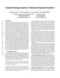
"name": "George Bluth", "age": 58, "indicted": true, "kids": ["Gob", "Lindsay", "Buster", { "name": "Michael", "age": 38, "kids": ["George-Michael"] }], "rival": "Stan Sitwell" } "name": "age": "charity_giving": "kids":

"Stan Sitwell", "middle-aged", 250120.5, ["Sally"] }

Figure 1: A pair of valid JSON objects.

2. BACKGROUND 2.1 The JSON Data Model The JSON data model [8] consists of four primitive types, and two structured types. The four primitive types are: • • • •

Unicode Strings, wrapped in quote characters. Numbers, which are double-precision IEEE floats. Boolean values, which are true or false. Null, to denote a null value.

The two structured types are: • Objects, which are collections of attributes. Each attribute is a key (String) and value (any type) pair. • Arrays, which are ordered lists of values. Values in an array are not required to have the same type. A value in an object or array can be either a primitive type or a structured type. Thus, JSON allows arbitrary nesting of arrays and objects. Figure 1 shows an example of two JSON objects. The first object has string attributes name and rival, a numeric age attribute, and a boolean indicted attribute. The object also has an attribute kids, which is an array consisting of three strings and an object (it is perfectly legal to mix value types in an array). The nested object in the kids array defines its own mapping of keys to values, and includes its own array of kids (recall that JSON can nest objects and arrays arbitrarily deep within each other).

2.2 JSON Document Stores JSON-based NoSQL document stores, such as MongoDB [2] and CouchDB [5], store collections of JSON objects in lieu of relational tables, and use JSON as the primary data format to interact with applications. There are no restrictions on the format and content of the objects stored, other than those imposed by the JSON standard. This leads to several salient differences from the relational model, namely: • Flexibility and Ease-of-Use: Since applications don’t have to define a schema upfront (or ever), application writers can quickly start working with the data, and easily adapt to changes in data structure. • Sparseness: An attribute with a particular key may appear in some objects in a collection, but not in others. This situation often arises in e-commerce data [4, 7]. • Hierarchical Data: Values may be arrays or objects, nested arbitrarily deep. In contrast to the relational approach of normalizing hierarchical data into separate ta-

bles with foreign-key references, hierarchical data is represented intensionally within the parent object [10]. • Dynamic Typing: Values for a particular key have no fixed data type, and may vary from object to object. MongoDB is the current market leader in the document store category, and has a richer feature set than CouchDB, including a real query language, secondary indices, and a fast binary representation of JSON [1]. MongoDB is used to power major web applications (including Craigslist, Foursquare, and bit.ly), content management systems (including LexisNexis and Forbes), and scientific data from the LHC [3].

2.3

JSON vs. XML

JSON is similar to XML in that both are hierarchical semistructured data models. In fact, JSON is replacing XML in some applications due to its relative simplicity, compactness, and the ability to directly map JSON data to the native data types of popular programming languages (e.g. Javascript). There is a rich body of research on supporting XML data using an underlying RDBMS. We are inspired by this research, and we have adapted some techniques originally proposed for dealing with XML to the JSON data model. We discuss the differences between XML and JSON in depth and draw insights from the existing XML research in [6].

3.

ARGO: BRINGING JSON TO RELATIONS

Existing NoSQL document stores are limited by the lack of a sophisticated and easy-to-use query language. The most feature-rich JSON-oriented query language today is MongoDB’s query language. It allows selection, projection, deletion, limited types of updates, and COUNT aggregates on a single collection of JSON objects, with optional ordering of results. However, there is no facility for queries across multiple collections (including joins), or for any aggregate function other than COUNT. Such advanced query constructs must be implemented outside of MongoDB, or within MongoDB by writing a Javascript MapReduce job (while in other systems like CouchDB, even simple queries require MapReduce). MongoDB’s query language requires specifying projection lists and predicates as specially-formatted JSON objects, which can make query syntax cumbersome. NoSQL systems typically offer BASE (basically available, soft state, eventually consistent) transaction semantics. The BASE model aims to allow a high degree of concurrency, but it is often difficult to program against a BASE model; for example, it is hard for applications to reconcile changes [11]. Recent versions of NoSQL systems such as MongoDB have made an effort to improve beyond BASE, but these improvements are limited to ensuring durability of individual writes and still fall far short of full ACID semantics. To address these limitations, we developed Argo, an automated mapping layer for storing and querying JSON data in a relational DBMS. Argo has two main components: • A mapping layer to convert JSON objects to relational tuples and vice versa. (Described in Section 3.1) • A SQL-like JSON query language, called Argo/SQL, for querying JSON data. Beneath the covers Argo/SQL converts queries to vanilla SQL that works with the mapping scheme, and reconstructs JSON objects from relational query results. (Described in Section 3.2) Note that since the Argo approach uses a relational engine, it can provide stronger ACID semantics.

3.1 Argo: The Mapping Layer The storage format of Argo handles schema flexibility, sparseness, hierarchical data, and dynamic typing as defined in Section 2.2. The Argo storage format was designed to be as simple as possible while still being a comprehensive solution for storage of JSON data, and is meant mainly to demonstrate the feasibility of storing JSON data in a relational system (We show in Section 5 that even this simple format provides good performance.) In order to address sparse data representation in a relational schema, Argo uses a vertical table format (inspired by [4]), with columns for a unique object id (a 64-bit BIGINT), a key string (TEXT), and a value. Rows are stored in vertical table(s) only when data actually exists for a key, which allows different objects to define values for different keys without any artificial restrictions on object schema, and without any storage overhead for “missing” values. To deal with hierarchical data (objects and arrays), we use a key-flattening approach. The keys of a nested object are appended to the parent key, along with the special separator character “.”. This technique has the effect of making the flattened key look like it is using the element-access operator, which is conceptually what it represents. Similarly, each value in an array is handled by appending the value’s position in the array to the key, enclosed by square brackets. This scheme allows the storage of hierarchical data in a single, flat keyspace. To illustrate, the flattened key for George Bluth’s grandson “George-Michael” in Figure 1 is kids[3].kids[0]. Key-flattening is similar to the Dewey-order approach for recording the order of XML nodes [13]. With the structured data types (objects and arrays) handled by key-flattening, we now address storage for the primitive types: strings, numbers, and booleans. We evaluated two storage schemes which we call Argo/1 and Argo/3. For the sake of brevity, we only describe Argo/3 in detail here, but full details on Argo/1 are available in [6].

3.1.1

Argo/3

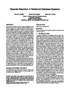
This mapping scheme uses three separate tables (one for each primitive type) to store a single JSON collection. Each table has the standard objid and keystr columns, as well as a value column whose type matches the type of data (TEXT for string, DOUBLE PRECISION for number, and BOOLEAN or BIT for boolean). This one-table-per-type schema is not unlike the use of different “node tables” to store element, attribute, and text nodes from an XML document in a relational system [12]. It is possible to store any number of JSON collections in just 3 tables by adding a column for a unique collection ID to this schema, but we do not do so because this can complicate query processing and cause data from a single collection to become sparse on shared data pages, incurring significant overhead. Figure 2 illustrates the Argo/3 representation for the sample JSON objects from Figure 1. All values in the two objects in the file are distributed across three tables, according to their types. In particular, the attributes with key age have different value types in the two objects, and therefore are separately stored in table argo people str and argo people num. Nested values are handled with key-flattening. To reconstruct JSON objects from the mapped tuples in this scheme, Argo starts with an empty JSON object and fetches rows from the three tables in parallel, ordered by objid. Argo examines the keystr of each row, checking for

objid 1 1 1 1 1 1 1 2 2 2

objid 1 1 2

argo people str keystr valstr name George Bluth kids[0] Gob kids[1] Lindsay kids[2] Buster kids[3].name Michael kids[3].kids[0] George-Michael rival Stan Sitwell name Stan Sitwell age middle-aged kids[0] Sally

argo people num keystr age kids[3].age charity giving

valnum 58 38 250120.5

argo people bool objid 1

keystr indicted

valbool true

Figure 2: Decomposition of JSON Objects from Figure 1 into the Argo/3 Relational Format. the element-access operator “.” and/or an array subscript in square brackets, creating intermediate nested objects or arrays as necessary on the path represented by the key string. The primitive value for the row (whose type depends on which of the three tables it was stored in) is inserted into the appropriate place in the reconstructed object. Argo repeats this process for all rows across the three tables which share the same objid. Argo then emits the reconstructed JSON object and starts over with a new, empty object, moving on to the next-lowest objid from the three tables.

3.2

Argo/SQL

Argo/SQL is a SQL-like query language for collections of JSON objects. It supports three types of statements: INSERT, SELECT, and DELETE. An insert statement has the following form: INSERT INTO collection_name OBJECT {...}; A SELECT statement can specify a projection list of attribute names or * for all attributes. It can optionally specify a predicate in a WHERE clause. It is also possible to specify a single INNER JOIN. To illustrate these features, we show a number of valid Argo/SQL SELECT statements, and the results they return, in Figure 3. We discuss the evaluation of predicates in Section 3.2.1, selection and projection in Section 3.2.2, and join processing in Section 3.2.3. Finally, a DELETE statement removes objects from a collection with an optional WHERE predicate. The following is an example of a valid DELETE statement in Argo/SQL: DELETE FROM people WHERE "Lindsay" = ANY kids; The above query deletes the first object from the collection. Note that it has a predicate that matches the string “Lindsay” with any of the values in the array kids. Arraybased predicates are discussed in more detail in Section 3.2.1. We describe the mechanics of selection query evaluation below. See [6] for more details on inserts and deletes.

3.2.1

Predicate Evaluation

Evaluating the WHERE clause of a SELECT or DELETE query requires a general mechanism for evaluating predicates on JSON objects and finding the set of objids that match. Simple Comparisons: Suppose we wish to evaluate a simple predicate comparing an attribute to a literal value. Argo selects objid from the underlying table(s) where keystr matches the specified attribute (values nested arbitrarily

Query SELECT age FROM people; SELECT * FROM people WHERE charity_giving > 100000;

SELECT left.name, right.kids FROM people AS left INNER JOIN people AS right ON (left.rival = right.name);

Result {"age": 58} {"age": "middle-aged"} { "name": "Stan Sitwell", "age": "middle-aged", "charity_giving": 250120.5, "kids": ["Sally"] } { "left": { "name": "George Bluth" }, "right": { "kids": ["Sally"] } }

Figure 3: Argo/SQL SELECT statement examples. deep in arrays or objects are allowed), and where the value matches the user-specified predicate. Argo uses the type of the literal value in such a predicate to determine which table to check against. The six basic comparisons (=, !=, =), as well as LIKE and NOT LIKE pattern-matching for strings, are supported. For example, the predicate charity_giving > 100000 is evaluated in Argo/3 as: SELECT objid FROM argo_people_num WHERE keystr = "charity_giving" AND valnum > 100000; Predicates Involving Arrays: Argo/SQL supports predicates that may match any of several values in a JSON array, using the ANY keyword. When ANY precedes an attribute name in a predicate, Argo will match any keystr indicating a value in the array, instead of exactly matching the attribute name. For example, the predicate "Lindsay" = ANY kids is evaluated in Argo/3 as: SELECT objid FROM argo_people_str WHERE keystr SIMILAR TO "kids\[[0123456789]+\]" AND valstr = "Lindsay"; Conjunctions: In general, an AND conjunction of predicates can not be evaluated on a single row of the underlying relational tables, since each row represents only a single value contained in an object. Fortunately, Argo can take the intersection of the matching objids for the subpredicates of a conjunction to find the matching objids for that conjunction. For example, the predicate age >= 50 AND indicted = True is evaluated in Argo/3 as: (SELECT objid FROM argo_people_num WHERE keystr = "age" AND valnum >= 50) INTERSECT (SELECT objid FROM argo_people_bool WHERE keystr = "indicted" AND valbool = true); Disjunctions: Just as a conjunction can be evaluated as the intersection of its child subpredicates, a disjunction can be evaluated as the UNION of the sets of objids matching its child subpredicates. For example, the predicate age >= 50 OR indicted = true is evaluated in Argo/3 as: (SELECT objid FROM argo_people_num WHERE keystr = "age" AND valnum >= 50) UNION (SELECT objid FROM argo_people_bool WHERE keystr = "indicted" AND valbool = true); Negations: Any basic comparison can be negated by taking the opposite comparison. For negations of conjunctions or disjunctions, Argo applies De Morgan’s laws to push negations down to the leaf comparisons of a predicate tree.

3.2.2

Selection

A SELECT query requires reconstruction of objects matching the optional predicate. If there is a WHERE predicate in a SELECT query, the matching object IDs (found via the

methods described in Section 3.2.1) are inserted into a temporary table (created with the SQL TEMPORARY keyword, so it is private to a connection), and attribute values belonging to the matching objects are retrieved via 3 SQL queries of the following form for each of the Argo/3 tables. SELECT * FROM argo_people_str WHERE objid IN (SELECT objid FROM argo_temp) ORDER BY objid; Argo iterates through the rows in the results of the above queries and reconstructs matching JSON objects according to the method described in Section 3.1.1. Projection: The user may wish to project only certain attributes from JSON objects matching a query, as illustrated in the first query in Figure 3. The object reconstruction algorithms detailed above are the same, with the addition of a predicate that matches only the specified attribute names. Because a given attribute may be an embedded array or object, we can not simply match the attribute name exactly, we must also find all nested child values if any exist. Argo accomplishes this task with LIKE predicates on the key string column. For example, if the projection list contains the attributes “name” and “kids”, Argo will run the following queries of the following form: SELECT * FROM argo_people_str WHERE (keystr = "name" OR keystr LIKE "name.%" OR keystr LIKE "name[%" OR keystr = "kids" OR keystr LIKE "kids.%" OR keystr LIKE "kids[%") AND objid IN (SELECT objid FROM argo_temp) ORDER BY objid;

3.2.3

Join Processing

Argo supports SELECT queries with a single INNER JOIN as illustrated by the last query in Figure 3. In order to evaluate a join condition on attributes of JSON objects, Argo performs a JOIN query on the underlying Argo/3 tables where the keystrs match the names of the attributes in the join condition, and the values satisfy the join condition. For example, to evaluate the JOIN query shown in Figure 3, Argo would run the following: SELECT argo_join_left.objid, argo_join_right.objid FROM argo_people_str AS argo_join_left, argo_people_str AS argo_join_right WHERE argo_join_left.keystr = "rival" AND argo_join_right.keystr = "name" AND argo_join_left.valstr = argo_join_right.valstr; This is not the end of the story, however, as many join conditions make sense for more than one of the JSON primitive data types. The equijoin shown above evaluates the join condition for strings. To evaluate the condition for numbers and boolean values, Argo runs two more queries similar to the above on the number and boolean tables, then takes the UNION of the three. As with a simple SELECT query, Argo stores the results of the above in a TEMPORARY intermediate table. Argo then selects rows matching the left and right objid in the intermediate table from the underlying data tables (optionally projecting out only certain attributes as described in Section 3.2.2), and reconstructs the joined objects according to the method described in Section 3.1.1.

4.

NOBENCH: A JSON BENCHMARK

NoBench is a micro-benchmark that aims to identify a simple and small set of queries that touch on common op-

erations in the target JSON settings. The NoBench queries are not meant to replicate or simulate a particular production workload, but instead focus on individual operations common to many applications. NoBench consists of a data generator and a set of 12 simple queries described below.

4.1 Generated Data The NoBench data generator creates a series of JSON objects with several attributes, including unique strings, numbers, dynamically typed attributes, a nested array of strings drawn from a Zipfian distribution of real English text [9], a small nested object, and several sparse attributes (each individual object has a set of 10 sparse attributes defined out of 1000 possible). See [6] for more details.

4.2 Queries The benchmark has twelve queries, and the result of each query is inserted into a temporary collection. The queries are grouped into five categories, and are described below. For more details, please see [6]. Projection - Q1 to Q4: These four projection queries run over all objects in the collection. Q1 projects common attributes, Q2 projects nested attributes from a nested object, and Q3 & Q4 project sparse attributes which only exist in a small number of objects. Selection - Q5 to Q9: Q5 is a rifle-shot selection query which selects one object by an exact match on a string attribute. Q6 through Q9 each select 0.1% of the objects in the collection, measuring the cost of reconstructing many matching objects with different types of predicates. Q6 uses a numeric predicate on a fixed-type numeric attribute, Q7 is similar but queries on a dynamically-typed attribute, Q8 matches a string in a nested array (simulating keyword search), and Q9 selects via a predicate on a sparse attribute. Aggregation - Q10: This query selects 10% of the objects in the collection, groups them into 1000 groups based on the value of a numeric attribute, and does a COUNT. Join - Q11: This query selects 0.1% of the objects in the collection and performs a self-equijoin of a nested string attribute with a non-nested string attribute. Since MongoDB has no native join facility, a Javascript MapReduce job was written to perform the join in MongoDB. Insert - Q12: This query bulk inserts 0.1% new data.

5. EVALUATION This section presents a sample of results of NoBench on a leading NoSQL database MongoDB (version 2.0.0), and Argo (see Section 3) on two representative open-source database systems PostgreSQL (version 9.1.1) and MySQL (version 5.5.15). Comprehensive results are available in [6]. We ran our experiments on a server with two Intel Xeon X5650 processors, 24GB of DDR3 main memory, and a hardware RAID-0 consisting of four 7200RPM disks. In all the experiments, we simply run one query at a time. In keeping with the design of the NoBench (a micro-benchmark), this method allows us to determine the performance of core data processing operations without other compounding factors. We configured all three systems as similarly as possible to ensure a fair comparison (all systems are configured to use up to 23 GB of memory, and have a checkpoint interval of five minutes and a group commit interval of 100 ms). Benchmark performance is sensitive to indexing. In all three systems, we created B-tree indices to enhance query

performance where sensible. In PostgreSQL and MySQL, we built indices on the objid and keystr columns of each of the three tables, as well as the valstr column of the string table and the valnum column of the number table. In MongoDB, indices are built on the values associated with a particular key. The MongoDB documentation recommends building indices to match queries that will actually be run, and we follow this recommendation, building indices on each non-sparse attribute which we query on. For each query, 10 runs, each with randomized parameters, are performed. We discard the maximum and minimum response times and report the mean time for the remaining 8 runs. With few exceptions, the normalized coefficient of variation in execution times was less than 20%, and tended to be smaller for longer-running queries. We use the mean time from MongoDB as a baseline. To compare the performance of Argo on MySQL and PostgreSQL with the MongoDB baseline, we calculate a unitless speedup factor, which is the mean execution time for MongoDB divided by the mean execution time for the other system. We also report the geometric mean of the speedup factors for all 12 queries. In order to study how the systems perform as the data size is scaled up, the queries in NoBench are evaluated over datasets whose cardinality is scaled by a factor of 4, from 1 million to 64 million objects. The total on-disk sizes of the datasets are reported in [6]. The 1-million and 4-million object datasets fit in memory for each database, while the 16 million object dataset exceeds the memory size for the relational systems (but not MongoDB), and the 64 million object dataset requires spilling to disk for all systems.

5.1

MongoDB vs. Argo

In this section, we present results from running NoBench on MySQL and PostgreSQL (with Argo/3), and MongoDB. Results are shown in Table 1. For the sake of space, we show only the smallest and largest scale factors. At each scale factor, the GM of speedup factors shows MySQL outperforming MongoDB. Argo on PostgreSQL outperforms MongoDB at the 1M and 4M scale factors, but falls somewhat behind at 16M and 64M. For all but the smallest scale, MySQL outperforms PostgreSQL. We perform a complete, detailed analysis of all queries, including analysis of the query plans chosen by each system’s optimizer, in [6]. To summarize, we found that a few major design differences between the systems had correspondingly major implications for performance: • Storage format: MongoDB stores whole objects contiguously using a fast binary representation of JSON [1]. Argo decomposes objects into a 1-row-per-value format. • Indices: indices in MongoDB are on the values of a particular attribute. Indices in Argo are built separately on objid, keystr, and various column values. MongoDB indices therefore tend to be smaller and are specialized to particular attributes. • MapReduce: MongoDB can’t natively query more than one table at once. Even a simple self-join (e.g. Q11) requires writing a Javascript MapReduce job, which can’t benefit from any indexing or native querying capability and requires frequent deserialization of JSON objects to load them into a Javascript VM. These factors limit the performance of MapReduce in MongoDB. We now summarize some key results from our evaluation: Projection: Argo on MySQL tends to outperform MongoDB for projection queries, as it can use an index on keystr

Projection

Selection

Aggregation Join Insert

Q1 Q2 Q3 Q4 Q5 Q6 Q7 Q8 Q9 Q10 Q11 Q12 GM

Mongo 104.56 102.95 3.24 3.53 1.59 1.76 1.58 1.66 1.90 1.24 211.81 0.19 1.0

1 Million Objects PGSQL Speedup MySQL 2.01 52.52 5.05 2.30 44.76 4.97 0.03 108.00 0.05 0.06 58.73 0.05 0.001 1590 0.001 0.06 29.33 0.17 0.05 31.60 0.11 0.05 33.20 0.11 0.17 11.18 0.47 0.85 1.46 2.28 16.69 12.69 0.16 0.83 0.23 1.30 – 23.90 –

Speedup 20.90 20.71 64.80 70.60 1590 10.35 14.36 15.09 4.04 0.54 1323.8 0.15 19.52

Mongo 7261.63 7276.17 472.05 553.92 260.73 353.10 321.47 326.38 362.65 31174.31 53318.21 35.12 1.0

64 Million Objects PGSQL Speedup MySQL 6004.00 1.21 1575.65 18913.28 0.38 1609.58 1811.96 0.26 514.90 1539.10 0.36 475.49 0.30 869.1 0.26 2993.52 0.12 2438.96 2239.01 0.14 1912.36 2975.56 0.11 1048.50 1800.08 0.20 1019.05 9479.01 3.29 2101.88 10117.21 5.27 2543.00 123.31 0.28 22.82 – 0.80 –

Speedup 4.61 4.52 0.92 1.16 1002.8 0.14 0.17 0.31 0.36 14.83 20.97 1.54 2.35

Table 1: Performance comparison. All times in seconds. Speedup column indicates speedup over MongoDB at the same scale factor (higher is better). GM is the geometric mean of the speedup factor over all queries. to quickly fetch just the appropriate rows, while MongoDB must scan every object and project attributes from each. Selection: For Q5 (rifle-shot selection), we found that MongoDB was using a scan to find the matching object, even though a clearly useful index was available (a serious oversight by the query optimizer). Argo on the SQL systems always uses an index to find the matching object, leading to its major performance advantage on Q5. For the 0.1% selectivity queries (Q6-Q9) MongoDB does use indices. At a scale of 1M objects, Argo on the relational systems outperforms MongoDB, but at larger scale factors MongoDB’s performance begins to overtake Argo. MongoDB benefits from more compact data storage and smaller, more specialized indices, requiring less disk I/O during query processing than Argo on MySQL or PostgreSQL for these queries. Aggregation: MongoDB’s built-in group function was used to implement COUNT with GROUP BY, and we found that MongoDB generally tends to outperform Argo on MySQL (though not overwhelmingly) for Q10 up through a scale factor of 16M. Once MongoDB’s data no longer fits in memory, however, we found that MongoDB switched from a relatively fast, optimized in-memory implementation of the group function to an extremely slow MapReduce version. Join: The join query, Q11, needs to use MapReduce on MongoDB, and much like the MapReduce version of Q10, the performance of this join query is far worse than Argo. Overall, our evaluation shows that when Argo/3 is run on MySQL, its performance is high enough to make it a compelling alternative to MongoDB. We find that, when data is small enough to fit entirely in memory, Argo/3 on MySQL outperforms MongoDB almost across the board. When data is too large to fit in memory, Argo/3 on MySQL has superior performance for all classes of queries except selection of large groups of objects, where MongoDB performs better.

6. CONCLUSION AND FUTURE WORK JSON document stores are rapidly gaining in popularity amongst developers of data-driven web and mobile applications, and traditional DBMSs are not being considered seriously in these new settings. In this paper, we have demonstrated with our prototype mapping layer Argo that traditional RDBMSs can support the flexibility of the schema-less JSON data model. Furthermore, one can go beyond what JSON NoSQL systems offer today and provide an easy-touse declarative query language. Our results demonstrate that the Argo solution is generally both higher performing

and more functional (e.g. it provides ACID guarantees and natively supports joins) than the leading NoSQL document store MongoDB. With Argo, traditional RDBMSs can offer an attractive alternative to NoSQL document stores while bringing additional benefits such as management tools that have been hardened for RDBMSs over time. There are a number of directions for future work, including expanding the evaluation to explore the impact of cluster environments, and looking at alternative mapping techniques (including encoding JSON objects as XML documents and using existing XML mappings). We hope that our initial work presented here will encourage a broader discussion about leveraging relational technology to support new applications using JSON data.

Acknowledgments This work was supported in part by the National Science Foundation under grants IIS-1110948 and IIS-1250886 and a gift donation from Google.

7.

REFERENCES

[1] 10Gen, Inc. BSON Specification. http://bsonspec.org/, 2011. [2] 10Gen, Inc. MongoDB. http://www.mongodb.org, 2011. [3] 10Gen, Inc. MongoDB Production Deployments. http://www.mongodb.org/display/DOCS/Production+Deployments, 2011. [4] R. Agrawal, A. Somani, and Y. Xu. Storage and querying of e-commerce data. In VLDB, pages 149–158, 2001. [5] Apache Software Foundation. Apache CouchDB. http://couchdb.apache.org/, 2011. [6] C. Chasseur, Y. Li, and J. M. Patel. Enabling JSON Document Stores in Relational Systems (Extended Paper). http://pages.cs.wisc.edu/~chasseur/argo-long.pdf. [7] E. Chu, J. Beckmann, and J. Naughton. The case for a wide-table approach to manage sparse relational data sets. In SIGMOD, pages 821–832. ACM, 2007. [8] D. Crockford. The application/json Media Type for JavaScript Object Notation (JSON). RFC 4627 (Informational), July 2006. [9] W. Francis and H. Kucera. A standard corpus of present-day edited american english. Department of Linguistics, Brown University, 1979. [10] E. Meijer and G. Bierman. A co-relational model of data for large shared data banks. Queue, 9:30:30–30:48, March 2011. [11] K. Muthukkaruppan. The Underlying Technology of Messages. Facebook’s Engineering Notes, 2010. [12] T. Shimura, M. Yoshikawa, and S. Uemura. Storage and retrieval of xml documents using object-relational databases. In DEXA, pages 206–217, 1999. [13] I. Tatarinov, S. D. Viglas, K. Beyer, J. Shanmugasundaram, E. Shekita, and C. Zhang. Storing and querying ordered xml using a relational database system. In SIGMOD, pages 204–215, 2002.