Jan Froehlich; Dolby Laboratories Inc.; Sunnyvale, USA & University of Stuttgart; Stuttgart, ... digital code words, as well as to find the number of code values.
Encoding Color Difference Signals for High Dynamic Range and Wide Gamut Imagery Jan Froehlich; Dolby Laboratories Inc.; Sunnyvale, USA & University of Stuttgart; Stuttgart, Germany Timo Kunkel; Dolby Laboratories Inc.; Sunnyvale, USA Robin Atkins; Dolby Laboratories Inc.; Sunnyvale, USA Jaclyn Pytlarz; Dolby Laboratories Inc.; Sunnyvale, USA Scott Daly; Dolby Laboratories Inc.; Sunnyvale, USA Andreas Schilling; University of Tübingen; Tübingen, Germany Bernd Eberhardt; Stuttgart Media University; Stuttgart, Germany
Abstract High dynamic range and wide color gamut are currently being introduced to television and cinema. This extended information requires not only more efficient signal encodings, but also improved color spaces. Due to the increasing variation in display capabilities, it is desirable to have a color signal encoding that is not only suitable for efficient quantization but also for color volume mapping. While an efficient method for high dynamic range luminance encoding has been put forward, a similar encoding scheme for color difference signals is not yet available. We address this with a novel color space representation that can be used for both efficient encoding of high dynamic range and wide gamut color difference signals as well as color volume mapping. We compare the performance, robustness and complexity against other color spaces in a variety of usage scenarios.
Introduction Luminance encoding for high dynamic range images has been studied extensively [1, 2]. There are also multiple proposals for high dynamic range color image encoding [3, 4, 5, 6, 7]. Common to all of these approaches is a focus on encoding efficiency; they are designed to be able to encode images using a minimum number of code values without introducing visible quantization artifacts or loss of image details. A modern image encoding scheme should not only be optimized for quantization but should also facilitate downstream steps like color volume mapping to prevent computationally expensive color space conversions for each step. Figure 1 depicts the full video distribution pipeline.
Unlike print media, digital cinema and television (TV) distribution did not typically require color volume mapping in the past because most display devices had a gamut and dynamic range that matched the encoded signal. A notable exception was early LCD displays that did not cover the complete Rec.709 [8] gamut. Future displays will have a larger variance in covered dynamic range and gamut. One reason for this is the trend toward mobile viewing, which extends potential ambient illumination from dark cinema and dim living rooms to bright sunlight for outside viewing. A second reason is that new display technologies have extended capabilities. Laser-illuminated projectors [9] are now becoming available and extend the gamut from DCI-P3 [10] to Rec.2020 [11]. At the same time, major TV networks are investigating how to distribute signals in Rec.2020 color space [12] to leverage the wider color gamut of emerging display technologies such as OLED [13], quantum dot displays [14] and already existing multi-primary displays [15, 16]. Most of these new displays and cinema projectors will not feature the full Rec.2020 gamut or the peak luminance of high dynamic range mastering displays. Thus, there will likely be more variation in device capabilities than ever before. This means that mapping between different color volumes will become critically important for consistent best-possible reproduction of TV and cinema imagery. In this paper, we co-optimize a color space for both high dynamic range (HDR) and wide color gamut (WCG) encoding efficiency as well as color volume mapping performance. In order to verify the efficiency of our color space, we compare it to state of the art HDR color encodings. Finally, we identify challenges associated with our approach and discuss further research opportunities.
Requirements
Figure 1. High dynamic range and wide color gamut distribution pipeline.
Thus, it is desirable to transmit video signals in an encoding color space that is not only suitable for efficient image encoding but also for tone and gamut mapping often referred to as color volume mapping.
240
The major goal of image encoding is to minimize color distortions when images are represented with a given number of digital code words, as well as to find the number of code values needed to prevent visible quantization artifacts. The best encoding performance is typically achieved when quantization error is distributed perceptually evenly over the color space. To fully avoid visible quantization errors, the step of one code value should always be below the detection threshold of one ‘just noticeable difference’ (JND). Thus, the more uniform in size the JND ellipsoids are throughout the color-space, the more efficient
© 2015 Society for Imaging Science and Technology
the encoding is, as there are less code values wasted to encode subJND steps in areas of the color space where JND-ellipsoids are larger [17]. We will denote this requirement as ‘JND-uniformity’. In addition to JND-uniformity, a color space for video encoding should decorrelate the achromatic axis from the chromatic axes to enable color subsampling that exploits the lower contrast sensitivity of the human visual system for high frequency chroma details. Furthermore, a color space used for color volume mapping should be as hue-linear as possible, as observers perceive changes in hue to be more impactful than changes in lightness or chroma. As such, most gamut mapping algorithms either completely avoid or heavily penalize hue changes. Thus, when mapping is performed toward the achromatic axis, or when intensity is changed, the color space should not introduce any hue changes. As well as maintaining uniformity inside the gamut volume, it is important to consider sufficiently large bounds to encode the necessary gamut and dynamic range. Rec.2020 gamut is the design goal for the next generation of displays and therefore the minimum requirement for a modern video encoding space. Short-term adaptive processes can expand the required dynamic range for entertainment imaging beyond the steady state adaptation of the human visual system [18]. A consumer study using an HDR research display in a dark viewing environment identified a dynamic range of 0.005-10000cd/m2 as required to satisfy 90% of the viewers [19]. Finally, the computational complexity of the transformation from the encoding color space to device RGB should be as low as possible to allow for mass deployment in a wide range of devices. Specifically the transformation should minimize computations in linear light and allow separable operations (i.e. functions of a single component rather than multiple components).
Prior Work One of the challenges in designing an efficient HDR color encoding is that in contrast to color appearance model expectations, neither surround luminance nor observer adaptation are known for HDR entertainment imaging scenarios. As a result, a static color difference formula designed for standard dynamic range like Delta-E 2000 [20] cannot be used to accurately predict JNDs. Instead, the quantization in any part of an HDR color space should always be determined by the adaptation parameters that result in the smallest detection step in that area to make sure visible quantization artifacts can be avoided for any content on any display in any viewing environment. The perceptual quantizer (PQ) curve [21] follows exactly this approach for luminance encoding. The PQ curve was derived as a constant minimum detectability curve from the Barten contrast sensitivity function (CSF) model [22] and is further predictable from a local cone model [23]. It always quantizes below the minimum contrast beyond the detection threshold for any adaptation state at any luminance. Figure 2 illustrates the concept of the PQ curve by comparing a range of theoretical cumulative JND curves for fixed steady state adaptation with the PQ-curve.
23rd Color and Imaging Conference Final Program and Proceedings
Figure 2. Minimum quantization for steady-state adaptation (red, green and blue lines) versus quantization determined by the minimum discriminability of all possible adaptation states (PQ / black dashed line).
Methods As our goal is a color difference encoding model that can be mass deployed, we chose an existing encoding scheme and searched for the optimal parameters of this model, rather than starting from scratch, without any constraints. The methods introduced here can also be used to optimize other models. In the following we will introduce the color space model and discuss the test and training sets and the cost functions we used for optimization of the model parameters.
Color Space Model We chose a color space model that follows the processing steps of broadcast video Y’CbCr and IPT [24]. As depicted in Formulas 1-3, this model consists of a linear transformation on device-dependent linear RGB followed by a nonlinear encoding function and a second linear transformation to decorrelate the nonlinear coded components into one achromatic channel and two color difference channels storing chroma information. !!"#$%" ! ! = !! ∙ ! !!"#$%" !!"#$%" ! !′ !′ = !!" !′
(1)
! ! ! !
(2)
! !′ !! = !! ∙ !′ !! !′
(3)
241
This model is easily invertible and already implemented in several hardware devices. In addition, IPT is known for its excellent hue linearity in standard dynamic range scenarios. The difference between Y’CbCr models and IPT is that in IPT the nonlinearity is applied to LMS cone fundamentals, rather than RGB primaries, and IPT uses a different color-differencing matrix compared to Y’CbCr. Both models have in common that intensity I and luma Y’ are not necessarily exactly weighted to the V-lambda luminosity function for all colors. Having chosen a specific model, we next search for the individual parameters of the model. At first, we determine the nonlinearity function (!!" ) by looking only at the achromatic axis. For Y’CbCr and IPT the achromatic case is true if all nonlinear components have the same value before applying the decorrelation matrix (!! ). From !!"!! (!) = ! = ! ! = ! ! we can deduce that if the optimal nonlinear encoding for I is known, this exact function also needs to be applied to !, ! and ! for quantization along the achromatic axis to be maximally efficient. The PQ curve shown in Formula 4 satisfies this requirement.
!!" :!!!!!!!!!" =
!! !!!
!! ! !""""
!!!!
!! ! !""""
!
!
!
(4)
where xl is the linear input and xnl is the nonlinear output. Further,!! = 2610/!2!" ,! !! = 2523/!2! , c1 = 3424/!2!" , c2 = 2413/ 2! !and c3 = 2392/ 2! )
The introduction of PQ as nonlinearity guarantees the quantization will be most efficient along the achromatic axis. However, the coefficients of matrix !! and !! cannot be directly deduced. Nonetheless, our model suggests some limitations that permit the reduction of free parameters. For matrix M1 the signal range for !, ! and ! should remain equal to the range of the input RGB because the nonlinear conversion function is only defined for zero to ten thousand. Thus the sum of the coefficients in each row of matrix !! must equal one. We can therefore reduce !! from 9 to 6 parameters !! to !! as shown in Formula 5. !! !! = !! !!
!! !! !!
1 − !! − !! 1 − !! − !! 1 − !! − !!
(5)
Matrix !! can also be reduced to six parameters. As intensity I is formed by the first row, !! and !! are the contributions of nonlinear encoded !′ and !′ to intensity. For peak-white, ! = !′ = ! !′ = ! !′! = 1 is true. Therefore, the sum of all upper row coefficients must again be 1. Thus, we can write the third coefficient of the first row as being dependent on !! and !! . The second and third rows of the color differencing matrix are calculated by subtracting I from !′ and !′, which mimics the classic color differencing approach from Y’CbCr or IPT and guarantees the chroma axes are orthogonal to the achromatic axis. The color-differencing matrix is followed by a free transform in the chroma domain via parameters s! to s! as shown in Formula 6. For easier visualization, we additionally rotate the chroma channels around the achromatic axis to make different optimization results comparable.
242
1 !! = 0 0
0 s! s!
!! 0 s! ∙ −!! s! 1 − !!
!! −!! −!!
1 − !! − !! !! + !! −1 + !! + !!
(6)
We will call the resulting intensity value I, and the two resulting color difference channels Ca and Cb. This naming is meant to reference the IPT and Y’CbCr models that inspired our model. Now that we have decided on a color encoding model and the nonlinearity function, we need to find parameters !! to !! , !! , !! and s! to s! . We chose to use optimization to find the matrix parameters because, unlike the nonlinearity function, they could not be directly deduced. The datasets and respective cost functions used to optimize the 12 parameters for hue-linearity, iso-luminance and uniform minimum discriminability are described in the following paragraphs.
Datasets Most existing datasets for hue linearity, iso luminance and discriminability are limited to standard dynamic range and a much smaller gamut compared to Rec.2020. Thus, we had to acquire our own datasets for optimization. This also allowed us to keep the training set (our data) separate from the verification set (existing data). The user study set-up for the acquisition of our data sets was kept as close as possible to existing studies; validity of the results could then be verified using the overlapping dynamic range and gamut regions. Equiluminant color pairs were acquired using the negativeface method [25] on a DLP-cinema projector equipped with modified notch-filters to allow sampling a near Rec.2020 color gamut. The projection size was adjusted to a diagonal of 50” to reach a peak white of 2000cd/m2. Constant hue lines were acquired from a user study that followed the setup of [26] in the modeling of hue uniformity for IPT with the exclusion of a reference gray patch but keeping the gray background and white border for anchoring. The results for stimuli inside Rec.709 gamut are very close to those from Hung and Berns [27] but our data extends to the full Rec.2020 gamut and beyond 100cd/m2. Threshold data for the detection criteria (JND) was acquired using a Dolby PRM4200 professional reference monitor with a black level of 0.005 cd/m2, a peak white of 600 cd/m2 and P3 gamut showing a step-edge pattern and using method of adjustment on the edge amplitude. For verification, we compared our findings with the JND ellipses of MacAdam [28] and Wright [29] as well as to the PQ curve and Kim’s contrast sensitivity function measurements [30].
Cost Functions For optimization of the 12 matrix parameters with the respective datasets, we needed to decide on cost functions. Our cost functions are defined as simply as possible because we found that the selection of the dataset and the weighting of the dataset samples have a greater influence on the results than the use of different reasonable cost functions. We defined the cost function for isoluminance (Cil) as the mean squared difference between the predicted intensity of colors adjusted by human observers to have the same perceived luminance. The isoluminance cost function is calculated in the
© 2015 Society for Imaging Science and Technology
nonlinear encoded domain of the respective color space and is shown in Formula 7. 1 !
!!!!!!!!!!!!!!!!!!!!!!!!!!!!!!!!!!!!!!!!!!!!" =
!
!!,! − !!,!
!
dealing with linear transformations, but because most JND ellipsoids are very small the error introduced by the nonlinearity is acceptable for our application.
!!!!!!!!!!!!!!!!!!!!!!!!!!!!!!(7)
!!!
where !!,! and !!,! are the intensities for n color pairs that were adjusted by human observers to have the same perceived luminance.
For hue linearity we defined the cost function (Chl) to be the difference between the predicted hue ℎ of each color in the hue linearity data set and the mean calculated hue of all samples adjusted by human observers to have the same perceived hue. This value is multiplied by saturation ! and normalized by the average saturation of all hues in the dataset to prevent the hue linearity cost function from having too much impact on the scaling of the final !! and !! values. The normalized differences are then squared and summed up for all samples. On its own, this hue linearity cost function always ends up at the trivial solution of projecting to a plane spanned by ! and one color vector. But because the later introduced JND-uniformity cost function (!!"# ) guarantees the color space will be near to uniform in JND size at all stages of optimization (except for the first few iterations), this hue-linearity cost function works without additional constraints. !!!!!!!!!!!!!!!!!!!ℎ!,! = atan2 !!,!,! , !!,!,! !!!!!!!!!!!!!!!!!!!!!!!!!!!!!!!!!!!!!!!!!!!!!!!!(8) !!!!!!!!!!!!!!!!!!!!!!,! = !
!!,!,!
1 !!!!!!!!!!!!!!!!!!!!!!" = !"
!
! !
!!! !!!
ℎ!,! − 1 !!!
1 ! ! !!!
! !!! ℎ!,! ! !!! !!,!
!
!!,!
Results and Verification !!!!!!!!!(10)
same perceived hue.
To generate the JND cost function (!!"# ) we first perform a singular value decomposition (SVD) on the ellipsoid half axes to ensure they are orthogonal after transformation to the current color space. After performing SVD, the sum of the squared differences between 1 and the length of the individual half axes (normalized by the average length of all half axes) is calculated. This is equivalent to variance in half-axes length with prior normalization. The entire cost function for JND uniformity is shown in Formula 11.
!!!!!!!!!!!!!"#
!
!
!!! !!!
!!!!!!!!!!!!!!!!!!!!!!!!!"!#$ = !!" !!" + !!" !!" + !!"# !!"# !!!!!!!!!!!!!!!!!! 12
+ !!,!,! !!!!!!!!!!!!!!!!!!!!!!!!!!!!!!!!!!!!!!!!!!!(9)
of m elements. Human observers adjusted all m elements of each tuple to have the
!
The total cost function (!!"!#$ ) is the sum of the weighted cost functions (Formula 12). Weighting allows us to manually adjust the trade-off between partly contradicting requirements like hue linearity and JND uniformity as noted below.
!
where hi,j and si,j are the hue and saturation in the new color space for n color tuples
1 = 3!
Figure 3. 2D example for JND ellipsoid representation as half axes.
!!,! 1 3!
! !!!
! !!!
!!,!
−1
!!!!!!!!!!!!!!(11)
where qi,j are the three half axes of n JND ellipsoids after singular value decomposition (SVD) has been applied to the half axes of each ellipsoid.
Figure 3 illustrates the half axes representation of a two dimensional ellipse and the need for singular value decomposition so that the length of the half axes again represents the maximum eccentricity of the ellipse after transformation to the current color space. In the case of typical color space conversion we are not only
23rd Color and Imaging Conference Final Program and Proceedings
The optimization process proved to be robust. When all 12 parameters were initialized with uniform distributed random values from their respective valid ranges, about 80% of the optimization runs converged to the same result (if rotation around the achromatic axis was ignored). As an example, Figure 4 shows the optimization results when changing the weighting of the cost function from JND uniformity towards hue linearity. The top row shows two samples from our hue linearity data set for observer JFR at the respective luminance of near Rec.2020 primaries for 185 and 1750cd/m2 peak white. A perfectly hue linear space would result in straight lines. The lower row shows samples from our JND dataset for observer JFR. In a color space that is perfectly uniform with respect to JND discriminability for this observer, and given no noise in the acquisition of the data, these ellipses will all be rendered as circles of uniform size. On the left side of Figure 4 hue nonlinearities are observed, especially the blue areas, while the JND-ellipses are rendered more uniform relative to the right side of the graph. On the right side of the figure hue linearity is greatly improved, but the ellipsoid in the blue area is less circular. Figures 4 indicates that balanced JND ellipsoids in the blue areas while retaining hue linearity in the blue area are not possible for our model. Lissner and Urban [31] suggest this issue is a fundamental problem for any color space model when trying to co-optimize for both JND uniformity and hue linearity.
243
Figure 4. Trading JND uniformity for hue-linearity by weighting the respective cost functions. Left: Optimization for JND uniformity results in curved hue lines, but more circular JND ellipses in the blue areas. Right: Optimization for hue linearity results in straight hue lines but a concave gamut shape and squeezed JND ellipsoids in the blue areas.
To verify the optimization process we compare one optimization result for our ICaCb model to current industry proposals for HDR color video encoding. For ICaCb the cost function weighting for hue-linearity versus JND uniformity is adjusted to yield a compromise between hue linearity and JNDuniformity. The conversion formula from CIE XYZ 1931 to the ICaCb model used in the comparison is given in equations 13 to 15. Valid input values include all XYZ values from a color space spanned by three primaries and D65 10,000 cd/m2 peak white (X = 9505, Y = 10,000 and Z = 10,891). 0.37613 ! ! = ! −0.21649 0.02567 !
0.70431 1.14744 0.16713!
!′, !′, !′ = ! 0.4949 !! = ! 4.2854 !! 0.3605
−0.05675! ! 0.05356! ∙ ! !0.74235! !
!! !!!
!,!,! ! !""""
!!!!
!,!,! ! !""""
0.5037 −4.5462 1.1499
!
(13)
!
!
0.0015 !′ 0.2609 ∙ !′ −1.5105 !′
(14)
(15)
where xl is the linear input and xnl is the nonlinear output. Further,!! = 2610/!2!" ,! !! = 2523/!2! , c1 = 3424/!2!" , c2 = 2413/ 2! !and c3 = 2392/ 2! )
Comparing this model with state of the art WCG and HDR encodings the International Telecommunication Union proposed using Rec.2020 primaries and a gamma curve with a linear toe followed by a color differencing matrix for next generation wide
244
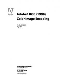
color gamut video [11]. However, if linearly scaled to a higher dynamic range, the quantization of the Rec.2020 gamma curve is too coarse in the dark areas and it ‘wastes’ code values in the bright areas. For this reason the BluRay Disc Association decided to replace the Rec.2020 gamma curve with PQ for the forthcoming UHD BluRay disk [5]. We refer to this encoding scheme as Rec.2020 PQ and compare it to the BBC proposal for HDR encoding [6], which is also based on Rec.2020 color primaries and the Rec.2020 color differencing matrix but uses a different nonlinear curve. The BBC curve is built by using a square root transformation below 100 cd/m2 and a natural logarithm transformation above. This encoding will be referred to as Rec.2020 BBC. The third candidate for comparison is Philips’ proposal for HDR and WCG video encoding called Y”u”v” [7]. Y”u”v” encodes luminance with the same PQ curve as Rec.2020 PQ and ICaCb, but encodes chroma as CIE 1976 u’v’. To reduce color noise, the u’v’ chromaticity coordinates are compressed for colors with luminance below about 5 cd/m2, and subsequently renamed to u’’ and v’’. Figure 5 shows the Rec.2020 1000cd/m2 peak white gamut hull for the above color spaces. On the left column the Hung and Berns hue linearity data set is overlaid to the gamut hull. ICaCb, Y’’u’’v’’ and Rec.2020 BBC perform better compared to Rec.2020 PQ for the luminance of the Hung and Berns data set. According to our hue-linearity data the hue curvature for Rec.2020 PQ and Rec.2020 BBC intensifies for higher luminance, especially in the blue areas while hue linearity for ICaCb and Y’’u’’v’’ stays about the same.
© 2015 Society for Imaging Science and Technology
The5.right of Figure 6 shows and Berns [27] hue background shows the Rec.2020 gamut hull at 1000cd/m peak white. The left Figure Visualrow verification of hue linearitythe andHung JND uniformity. The colored 2
column shows the Hung and Berns hue linearity data. Straight lines from the center indicate a more hue linear color space. The right column shows 10 times amplified MacAdam1942 PGN JND ellipses. The more regular the ellipses are in size the more uniform the space is in regards to JNDs.
23rd Color and Imaging Conference Final Program and Proceedings
245
For the visual verification of JND-uniformity, we selected those chromaticity ellipses from MacAdam’s PGN observer that are located inside the Rec.2020 gamut. The right column of Figure 5 shows these ellipses amplified by a factor of 10 in an orthographic view along the achromatic axis. ICaCb and Y’’u’’v’’ render the minimum discriminability ellipses more uniform than Rec.2020 PQ and Rec.2020 BBC. For numerical verification of the coding efficiency we built JND ellipsoids by replicating the MacAdam PGN ellipses to 0.02, 0.2, 2, 40 and 200 cd/m2 and scaling it by Kim’s color contrast sensitivity function findings [30] in the chromaticity domain relative to the 40 cd/m2 results. For the achromatic axis we multiplied Kim’s peak sensitivity findings by three to compensate for an assumed systematic error in the general scale of Kim’s achromatic contrast sensitivity function. As an example, the colorfest study [32] found the peak contrast sensitivity to be about three times more sensitive compared to Kim’s results. Including the multiplication, Kim’s peak contrast sensitivities aligned well with our JND study’s findings and the results from the verification of the PQ curve. Encoding efficiency can be calculated by dividing the needed range per axis by the largest allowed quantization step below the visibility threshold. We chose Rec.2020 1000 cd/m2 peak white gamut to determine the minimum and the maximum expected values per axis. In contrast to the minimum and maximum values, the largest visually lossless quantization step per axis cannot be separately determined because the needed quantization along one axis depends on the quantization along the other axes. As a result any quantization that is half the size of an axis-aligned box that fits inside all JND ellipsoids is visually lossless. Figure 6 illustrates two visually lossless quantization step sizes for the same JND ellipse.
trading quantization efficiency along the achromatic axis in favor of needed code values for chroma or vice versa. Table 1 compares the encoding efficiency for the investigated color spaces. 2
Table 1. Code values needed to encode Rec.2020 1000cd/m peak white gamut. Fewer code values indicate a more efficient encoding.
Luma Chroma 1 Chroma 2
Rec.2020 BBC Y’: 7009 Cb: 9432 Cr: 7554
Rec.2020 PQ Y’: 2816 Cb: 3526 Cr: 4342
Y’’u’’v’’
ICaCb
Y’’: 2370 u’’: 1829 v’’: 942
I : 2147 Ca: 1621 Cb: 832
Due to the PQ nonlinearity on the achromatic axis, ICaCb and Y’’u’’v’’ provide the most efficient luminance encoding. ICaCb and Y’’u’’v’’ also need less code values for chroma compared to the other color spaces we investigated. The high number of code values needed for Rec.2020 PQ results from the skewed JND ellipsoids for saturated colors while the high amount of code values for Rec.2020 BBC is due to the comparatively coarse quantization of the square-root curve in the dark areas.
Discussion The performance of the proposed ICaCb color space for encoding high dynamic range and wide gamut video and performing color volume mapping is very promising. In addition to the visual and numerical analyses, we performed gamut mapping and tone mapping using the wide gamut scenes from the HdMHDR-2014 dataset [33] as well as a custom database of wide color gamut and high dynamic range image sequences. ICaCb was found to be very robust without showing typical problems like the huenonlinearity in the blues. In future it would be desirable to evaluate and eventually reoptimize the transformation matrices with a wider data set. As an example, we plan to repeat our minimum JND study on a Rec.2020 capable display and use a more robust psychometric method such as two-alternative forced choice instead of the method of adjustment that was utilized in our first minimum JND study. The ICaCb color space should also be evaluated for compression efficiency to provide a solution beyond baseband encoding of uncompressed image streams.
Conclusion Figure 6. Deriving the largest possible visually lossless quantization from JND ellipses. To make sure any change in color is below the detection threshold any combination of one code value change along all axes must fall inside the JND ellipse. Thus, coarse quantization steps on axis 2 of the left plot results in fine quantization steps needed for axis 1 while a finer resolution on the second axis of the right plot allows the first axis to be quantized in coarser steps.
To determine minimum quantization, we evenly scaled the axis-aligned bounding-boxes of each ellipsoid to fit inside the respective ellipsoid. The needed quantization step was then determined by the minimum of half the length of all boxes along each of the three axes. As illustrated in Figure 6, different approaches can result in slightly different results, for example
246
We introduce a new color space for encoding high dynamic range and wide gamut video. This color space builds on proven transformations and is co-optimized for encoding efficiency and color volume mapping applications. Consequently, it provides optimized encoding performance for high dynamic range and wide gamut imagery and helps provide efficient implementations for tone- and gamut mapping that will be needed for most display devices in the future.
References [1]
National Electrical Manufacturers Association, “Digital Imaging and Communications in Medicine (DICOM) Part 14: Grayscale Standard Display Function (PS 3.14-2011),” Rosslyn, USA, 2004.
© 2015 Society for Imaging Science and Technology
[2]
M. Nezamabadi, S. Miller, et al., "Color signal encoding for high dynamic range and wide color gamut based on human perception, " IS&T/SPIE Electronic Imaging, San Francisco, USA, 2014.
[19] S. Daly, T. Kunkel, et al., "Preference limits of the visual dynamic range for ultra high quality and aesthetic conveyance," IS&T/SPIE Electronic Imaging, Burlingame, CA, USA, 2013.
[3]
G. Ward, "The RADIANCE Lighting Simulation and Rendering System, " Association for Computing Machinery (ACM) SIGGRAPH, Orlando, USA, 1994.
[20] M. R. Luo, et al. "The development of the CIE 2000 colour!difference formula: CIEDE2000," Color Research & Application, vol. 26, no. 5 pp 340-350, 2001.
[4]
G. Ward, "LogLuv encoding for full-gamut, high-dynamic range images," Journal of Graphics Tools, vol. 3, no. 1, pp. 15-31, 1998.
[5]
Blu-ray Disc Association, "Coding constraints on HEVC video streams for BD-ROM Version 3.0," Burbank, USA, 2015.
[21] J.S. Miller, M. Nezamabadi, and S. Daly, Society of Motion Picture & Television Engineers (SMPTE), ST-2084 „High Dynamic Range Electro-Optical Transfer Function of Mastering Reference Displays,“ SMPTE, White Plains, USA, 2014.
[6]
A. Cotton and T. Borer, "BBC’s response to CfE for HDR Video Coding (Category 3a)", ISO/IEC JTC1/SC29/WG11 M36249, Warsaw, Poland, 2015.
[7]
C. Poynton, J. Stessen et al., "Deploying wide colour gamut and high dynamic range in HD and UHD," SMPTE Motion Imaging Journal, vol. 124, no 3, pp. 37-49, 2015.
[8]
International Telecommunication Union (ITU), Recommendation ITU-R BT.709-5 "Basic Parameter Values for the HDTV Standard for the Studio and for International Programme Exchange," Geneva, Switzerland, 2002.
[9]
B. D. Silverstein, A. F. Kurtz, et al., "A Laser-Based Digital Cinema Projector," Society for Information Display (SID) Symposium, Los Angeles, USA, 2011
[10] Society of Motion Picture & Television Engineers (SMPTE), ST-4312 "D-Cinema Quality - Reference Projector and Environment," SMPTE Technology Committee DC28 on D-Cinema, White Plains, USA, 2011. [11] International Telecommunication Union (ITU), Recommendation ITU-R BT.2020-1 "Parameter Values for Ultra-High Definition Television Systems for Production and International Programme Exchange," Geneva, Switzerland, 2014. [12] M. Pedzisz, "Beyond BT. 709," Society of Motion Picture & Television Engineers (SMPTE) Motion Imaging Journal vol. 123, no. 8, pp. 18-25, 2014.
[22] P. G. J. Barten, "Formula for the contrast sensitivity of the human eye." SPIE Electronic Imaging 2004. San Jose, CA, USA, 2004. [23] S. Daly and S. A. Golestaneh, "Use of a local cone model to predict essential CSF light adaptation behavior used in the design of luminance quantization nonlinearities," IS&T/SPIE Electronic Imaging, San Francisco, CA, USA, 2015. [24] F. Ebner and M. D. Fairchild. "Development and testing of a color space (IPT) with improved hue uniformity," IS&T Color and Imaging Conference, Scottsdale, AZ, USA, 1998. [25] G. Kindlmann, E. Reinhard, et al. "Face-based luminance matching for perceptual colormap generation," IEEE Conference on Visualization, Boston, MA, USA, 2002. [26] F. Ebner, “Derivation and Modeling of Hue Uniformity,” PhDThesis, Rochester Institute of Technology, Rochester, NY, USA, 1998. [27] P.C. Hung and R. S. Berns, "Determination of constant hue loci for a CRT gamut and their predictions using color appearance spaces," Color Research & Application, vol. 20, no. 5, pp. 285-295, 1995. [28] D. L. MacAdam "Visual sensitivities to color differences in daylight." Journal of the Optical Society of America, vol. 32, no.5, pp. 247-273, 1942. [29] W. D. Wright, "The sensitivity of the eye to small colour differences," Proceedings of the Physical Society, vol. 53, no. 2, pp. 93, 1941.
[13] D. M. Hoffman, et al. "240 Hz OLED technology properties that can enable improved image quality," Journal of the Society for Information Display, vol. 22, no. 7, pp. 346-356 2014.
[30] K. J. Kim, R. Mantiuk, et al. "Measurements of achromatic and chromatic contrast sensitivity functions for an extended range of adaptation luminance," IS&T/SPIE Electronic Imaging, Burlingame, CA, USA, 2013.
[14] A. Ninan, "Impacting the Display Industry Through Advances in Next Generation Video," Society for Information Display (SID) Display Week, San Diego, CA, 2014.
[31] Ingmar Lissner and Philipp Urban, "How perceptually uniform can a hue linear color space be?" IS&T Color and Imaging Conference, San Antonio, TX, USA, 2010.
[15] S. Roth, N. Weiss, et al., "Multi-Primary LCD for TV Applications, Genoa Color Technologies," Society for Information Display (SID) Symposium, Long Beach, CA, USA, 2007.
[32] S. M. Wuerger, A. B. Watson, et al., "Towards a spatio-chromatic standard observer for detection," IS&T/SPIE Electronic Imaging, San Jose, CA, USA, 2002.
[16] S. Ueki, K. Nakamura, et al., "Five-primary-color 60-inch LCD with Novel Wide Color Gamut and Wide Viewing Angle," Society for Information Display (SID) Symposium, San Antonia, TX, USA, 2007.
[33] J. Froehlich, S. Grandinetti, et al., "Creating cinematic wide gamut HDR-video for the evaluation of tone mapping operators and HDRdisplays," IS&T/SPIE Electronic Imaging, San Francisco, CA, USA, 2014.
[17] T. Kunkel, G. Ward, et al., "HDR and Wide Gamut Appearancebased Color Encoding and its Quantification," 30th IEEE Picture Coding Symposium, San Jose, CA, USA, 2013.
Author Biography
[18] T. Kunkel and E. Reinhard. "A reassessment of the simultaneous dynamic range of the human visual system," Association for Computing Machinery (ACM) Symposium on Applied Perception in Graphics and Visualization, Los Angeles, CA, USA, 2010.
23rd Color and Imaging Conference Final Program and Proceedings
Jan Froehlich (born 1979 in Germany) is currently a Ph.D.-student at the University of Stuttgart. He is working on high dynamic range and wide color gamut imaging as well as gamut mapping. Before beginning his Ph.D. he was Technical Director at CinePostproduction GmbH in Germany. He is member of IS&T, SMPTE, SPIE, FKTG, and the German Society of Cinematographers (BVK).
247