applied sciences Article
SampleCNN: End-to-End Deep Convolutional Neural Networks Using Very Small Filters for Music Classification† Jongpil Lee, Jiyoung Park, Keunhyoung Luke Kim and Juhan Nam * Graduate School of Culture Technology, KAIST, 291 Daehak-ro, Yuseong-gu, Daejeon 34141, Korea;
[email protected] (J.L.);
[email protected] (J.P.);
[email protected] (K.L.K.) * Correspondence:
[email protected]; Tel.: +82-42-350-2926 † This article is a re-written and extended version of “Sample-level Deep Convolutional Neural Networks for music auto-tagging using raw waveforms” presented at SMC 2017, Espoo, Finland on 5 July 2017. Academic Editor: Meinard Müller Received: 3 November 2017; Accepted: 17 January 2018; Published: 22 January 2018
Abstract: Convolutional Neural Networks (CNN) have been applied to diverse machine learning tasks for different modalities of raw data in an end-to-end fashion. In the audio domain, a raw waveform-based approach has been explored to directly learn hierarchical characteristics of audio. However, the majority of previous studies have limited their model capacity by taking a frame-level structure similar to short-time Fourier transforms. We previously proposed a CNN architecture which learns representations using sample-level filters beyond typical frame-level input representations. The architecture showed comparable performance to the spectrogram-based CNN model in music auto-tagging. In this paper, we extend the previous work in three ways. First, considering the sample-level model requires much longer training time, we progressively downsample the input signals and examine how it affects the performance. Second, we extend the model using multi-level and multi-scale feature aggregation technique and subsequently conduct transfer learning for several music classification tasks. Finally, we visualize filters learned by the sample-level CNN in each layer to identify hierarchically learned features and show that they are sensitive to log-scaled frequency. Keywords: convolutional neural networks; music classification; raw waveforms; sample-level filters; downsampling; filter visualization; transfer learning
1. Introduction Convolutional Neural Networks (CNN) have been applied to diverse machine learning tasks. The benefit of using CNN is that the model can learn hierarchical levels of features from high-dimensional raw data. This end-to-end hierarchical learning has been mainly explored in the image domain since the break-through in image classification [1]. However, the approach has been recently attempted in other domains as well. In the text domain, a language model is typically built in two steps, first by embedding words into low-dimensional vectors and then by learning a model on top of the word-level vectors. While the word-level embedding plays a vital role in language processing [2], it has limitations in that the embedding space is learned separately from the word-level model. To handle this problem, character-level language models that learn from the bottom-level raw data (e.g., alphabet characters) were proposed and showed that they can yield comparable results to the word-level learning models [3,4]. In the audio domain, raw waveforms are typically converted to time-frequency representations that better capture patterns in complex sound sources. For example, spectrogram and more concise
Appl. Sci. 2018, 8, 150; doi:10.3390/app8010150
www.mdpi.com/journal/applsci
Appl. Sci. 2018, 8, 150
2 of 14
representations such as mel-filterbank are widely used. These spectral representations have served a similar role to the word embedding in the language model in that the mid-level representation are computed separately from the learning model and they are not particularly optimized for the target task. This issue has been addressed by taking raw waveforms directly as input in different audio tasks, for example, speech recognition [5–7], music classification [8–10] and acoustic scene classification [11,12]. However, the majority of previous work have focused on replacing the frame-level time-frequency transforms with a convolutional layer, expecting that the layer can learn parameters comparable to the filter banks. The limitation of this approach was pointed out by Dieleman and Schrauwen [8]. They conducted an experiment of music classification using a simple CNN that takes raw waveforms or mel-spectrogram. Unexpectedly, their CNN models with the raw waveform as input did not produce better results than those with the spectral data as input. The authors attributed this unexpected outcome to three possible causes. First, their CNN models were too simple (e.g., a small number of layers and filters) to learn the complex structure of polyphonic music. Second, the end-to-end models need an appropriate non-linearity function that can replace the log-based amplitude compression in the spectrogram. Third, the first 1D convolutional layer takes raw waveforms in a frame-level which is typically several hundred samples long. The filters in the first 1D convolutional layer should learn all possible phase variations of periodic waveforms within the length. In spectrogram, the phase variation is removed. We recently tackled the issues by stacking 1D convolutional layers using very small filters instead of a 1D convolutional layer with the frame-level filters, inspired by the VGG networks in image classification that is built with deep stack of 3×3 convolutional layers [13,14]. The sample-level CNN model has filters with very small granularity (e.g., 3 samples) in time for all convolutional layers. The results were comparable to those using mel-spectrogram in music auto-tagging. In this paper, we term the sample-level CNN architecture as SampleCNN and extend the previous work in three ways. First, we should note that SampleCNN takes four times longer training time than a comparable CNN model that takes mel-spectrogram. In order to reduce the training time, we progressively downsample the waveforms and report the effect on performance. By reducing the band-width of music audio this way, we will be able to find the cut-off frequency where the performance starts to become degraded. Second, we extended SampleCNN using multi-level and multi-scale feature aggregation [15]. The technique proved to be highly effective in music classification tasks. We additionally evaluate the extended model in transfer learning settings where the features extracted from SampleCNN can be used for three different datasets in music genre classification and music auto-tagging. We show that the proposed model achieves state-of-the-art results. Third, we visualize learned intermediate layers of SampleCNN to observe how the filters with small granularity process music signals in a hierarchical manner. In particular, we visualize them for each of sampling rates. 2. Related Work There are a decent number of CNN models that take raw waveforms as input. The majority of them used large-sized filters in the first convolutional layer with various size of strides to capture frequency-selective responses which were carefully designed to handle their target problems. We termed this approach as frame-level raw waveform model because the filter and stride sizes of the first convolutional layer were chosen to be comparable to the window and the hop sizes of short-time Fourier transformation, respectively [5–11]. There are a few work that used small filter and stride sizes in the first convolution layer (8 samples-sized filter [16] and 10 samples-sized filter [17,18] at 16 kHz). However, the CNN models have only two or three convolution layers, which are not sufficient to learn the complex structure of the acoustic signals. In SampleCNN, we deepen the layers even more, thereby reducing the filter and stride sizes of the first convolution layer down to two or three samples.
Appl. Sci. 2018, 8, 150
3 of 14
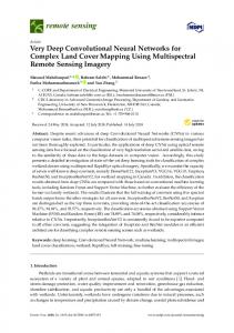
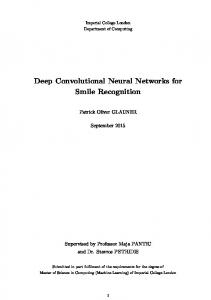
3. Learning Models Figure 1 illustrates three CNN models in music auto-tagging that we compare in our experiments. Note that they are actually general architectures and so can be applied to any audio classification tasks. In this section, we describe the three models in detail.
Figure 1. Comparison of (a) frame-level model using mel-spectrogram; (b) frame-level model using raw waveforms and (c) sample-level model using raw waveforms.
3.1. Frame-Level Mel-Spectrogram Model This is the most common CNN model used in music classification. The time-frequency representation is usually regarded as either two-dimensional images [19,20] or one-dimensional sequence of vectors [8,21]. We only used one-dimensional(1D) CNN model for experimental comparisons because the performance gap between 1D and 2D models is not significant and the 1D model is directly comparable to models using raw waveforms. 3.2. Frame-Level Raw Waveform Model In this model, a strided convolution layer is added beneath the bottom layer of the frame-level mel-spectrogram model. The strided convolution layer is expected to learn a filter-bank that returns a time-frequency representation. In this model, once the first strided convolution layer slides over the raw waveforms, the output feature map has the same dimensions as the mel-spectrogram. This is because the stride size, filter size, and the number of filters in the first convolution layer correspond to the hop size, window size, and the number of mel-bands in the mel-spectrogram, respectively. This configuration was used for the music auto-tagging task in [8,9] and thus we used it as a baseline model. 3.3. Sample-Level Raw Waveform Model: SampleCNN As described in Section 1, the approach using raw waveforms should be able to address log-scale amplitude compression and phase-invariance. Simply adding a strided convolution layer is not sufficient to overcome the issues. To improve this, we add multiple layers beneath the frame-level such that the first convolution layer can handle much smaller size of samples. For example, if the stride of the first convolution layer is reduced from 729 (=36 ) to 243 (=35 ), 3-size convolution layer and max-pooling layer are added to keep the output dimensions in the subsequent convolution layers unchanged. If we repeatedly reduce the stride of the first convolution layer this way, six convolution
Appl. Sci. 2018, 8, 150
4 of 14
layers (five pairs of 3-size convolution and max-pooling layer following one 3-size strided convolution layer) will be added (we assume that the temporal dimensionality reduction occurs only through max-pooling and striding while zero-padding is used in convolution to preserve the size). We generalized the configuration as mn -SampleCNN where m refers to the filter size (or the pooling size) of intermediate convolution layer modules and n refers to the number of the modules. The first convolutional layer is different from the intermediate convolutional layers in that the stride size is equal to the filter size. An example of mn -SampleCNN is shown in Table 1 where m is 3 and n is 9. Note that the network is composed of convolution layers and max-pooling only, and so the input size is determined to be stride size of the first convolutional layer ×mn . In Table 1, as the stride size of the first convolution layer is 3, the input size is set to be 59049 (=3 × 39 ). Table 1. SampleCNN configuration. In the first column (Layer), “conv 3-128” indicates that the filter size is 3 and the number of filters is 128. 39 -SampleCNN Model 59,049 Samples (2678 ms) as Input Layer
Stride
Output
# of Params
conv 3-128
3
19,683 × 128
512
conv 3-128 maxpool 3
1 3
19,683 ×128 6561 × 128
49,280
conv 3-128 maxpool 3
1 3
6561 × 128 2187 × 128
49,280
conv 3-256 maxpool 3
1 3
2187 × 256 729 × 256
98,560
conv 3-256 maxpool 3
1 3
729 × 256 243 × 256
196,864
conv 3-256 maxpool 3
1 3
243 × 256 81 × 256
196,864
conv 3-256 maxpool 3
1 3
81 × 256 27 × 256
196,864
conv 3-256 maxpool 3
1 3
27 × 256 9 × 256
196,864
conv 3-512 maxpool 3
1 3
9 × 512 3 × 512
393,728
conv 3-512 maxpool 3
1 3
3 × 512 1 × 512
786,944
conv 1-512 dropout 0.5
1 −
1 × 512 1 × 512
262,656
sigmoid
−
50
25,650
Total params
2.46 × 10⁶
4. Extension of SampleCNN 4.1. Multi-Level and Multi-Scale Feature Aggregation Music classification tasks, particularly music auto-tagging among others, have a wide variety of labels in terms of genre, mood, instruments and other song characteristics. Especially, they are positioned in different hierarchical levels and time-scales. For example, some words related to instrument ones, such as guitar and saxophone, describe objective sound sources which are usually local and repetitive within a song, whereas other labels related to genre or mood, such as rock and
Appl. Sci. 2018, 8, 150
5 of 14
happy, are dependent on a larger context of music and are more complicated. In order to address this issue, we recently proposed multi-level and multi-scale feature aggregation technique [15]. The technique is conducted by combining multiple CNN models. This assumes that the hidden layers of each CNN model represent different levels of features and the models with different input sizes provide even richer feature representations by capturing both local and global characteristics of the music. In [15], they showed that different level and time-scale features have different performance sensitivity to individual tags and thus combining them all together is the best strategy to improve performance. In this work, we replace the simple CNN architectures that take mel-spectrogram as input in [15] with SampleCNNs, taking different input sizes (e.g., 700 ms to 3.5 s). Once we train the SampleCNNs as supervised feature extractors, we slide each of them over a song clip (e.g., about 30 s) and obtain features from the last three hidden layers. We then summarize them by a combination of max-pooling and average-pooling. Finally, we concatenate the multi-level and multi-scale features and feed them to a simple neural networks with two fully-connected layers to make a final prediction. 4.2. Transfer Learning The multi-level and multi-scale feature aggregation approach can be used in a transfer learning setting by using different datasets or target tasks for the final classification after training the SampleCNNs. Especially, when the target dataset size is comparably small to the model capacity, transferred parameters can yield better performance on the target task rather than parameters trained from the innate target dataset. The applicability of transfer learning using a frame-level raw waveform model has been explored in the speech domain [17]. Here, we examine it using the sample-level raw waveform model for music genre classification and music auto-tagging with different datasets. 5. Experimental Setup 5.1. Datasets We validate the effectiveness of the proposed method on different sizes of datasets for music genre classification and auto-tagging. All dataset splits are available on the link [22]. The details of each dataset are as follows. The numbers in the parenthesis indicate the split of training, validation and test sets. • • •
•
GTZAN [23]: 930 songs (443/197/290) (This is a fault-filtered split designed to avoid the repetition of artists across the training, validation and test sets [24]), genre classification (10 genres). MagnaTAgaTune (MTAT) [25]: 21,105 songs (15,244/1529/4332), auto-tagging (50 tags) Million Song Dataset with Tagtraum genre annotations (TAGTRAUM): 189,189 songs (141,372/10,000/37,817) (This is a stratified split with 80% training data of the CD2C version [26]), genre classification (15 genres) Million Song Dataset with Last.FM tag annotations (MSD) [27]: 241,889 songs (201,680/11,774/28,435), auto-tagging (50 tags)
We primarily examined the proposed model on MTAT and then verified the effectiveness of our model on MSD which is much larger than MTAT (MTAT contains 170 h long audio and MSD contains 1955 h long audio in total). We filtered out the tags and used most frequently labeled 50 tags in both datasets, following the previous work [8,19,20]. Also, all songs in the two datasets were trimmed to 29.1 s long. For transfer learning experiments, the model is first trained with the largest dataset, MSD, and the pre-trained networks are transferred to other three datasets. The evaluation is conducted with area under receiver operating characteristic (AUC) for auto-tagging datasets and accuracy for genre classification datasets.
Appl. Sci. 2018, 8, 150
6 of 14
5.2. Training Details We used sigmoid activation for the output layer and binary cross entropy loss as the objective function to optimize. For every convolution layer, we used batch normalization [28] and ReLU activation. We should note that, in our experiments, batch normalization plays a vital role in training the deep models that take raw waveforms. We applied dropout of 0.5 to the output of the last convolution layer and minimized the objective function using stochastic gradient descent with 0.9 Nesterov momentum. The learning rate was initially set to 0.01 and decreased by a factor of 5 when the validation loss did not decrease more than 3 epochs. A total decrease of 4 times, the learning rate of the last training was 0.000016. Also, we used batch size of 23 for MTAT and 50 for MSD, respectively. 5.3. Mel-Spectrogram and Raw Waveforms In the mel-spectrogram experiments, window sizes of 36 , 35 and 34 are used to match up to the filter sizes in the first convolution layer of the raw waveform model as shown in Table 2. FFT size was set to 729 (=36 ) in all experiments. When the window is less than the FFT size, we zero-padded the windowed frame. The linear frequency in the magnitude spectrum is mapped to 128 mel-bands and the magnitude compression is applied with a nonlinear curve, log(1 + C | A|) where A is the magnitude and C is set to 10. Also, we conducted the input normalization simply by dividing the standard deviation after subtracting mean value of entire input data. On the other hand, we did not perform the input normalization for raw waveforms. Table 2. Comparison of three CNN models with different window size (filter size) and hop size (stride size). n represents the number of intermediate convolution and max-pooling layer modules, thus 3n times hop (stride) size of each model is equal to the number of input samples. 3n Models, 59,049 Samples as Input
n
Window Size (Filter Size)
Hop Size (Stride Size)
AUC
Frame-level (mel-spectrogram)
4 5 5 6 6
729 729 243 243 81
729 243 243 81 81
0.9000 0.9005 0.9047 0.9059 0.9025
4 5 5 6 6 7 8 9
729 729 243 243 81 27 9 3
729 243 243 81 81 27 9 3
0.8655 0.8742 0.8823 0.8906 0.8936 0.9002 0.9030 0.9055
Frame-level (raw waveforms)
Sample-level (raw waveforms)
As described in Section 3.3, m refers to the filter size (which can be compared to a window size of FFT in the spectrogram) or pooling size (which also can be compared to a hop size of FFT in the spectrogram) of the intermediate convolution layer modules, and n refers to the number of the modules. In our previous work, we adjusted m from 2 to 5 and increased n according to the configuration of mn -SampleCNN [13]. Among them, 39 -SampleCNN model with 59049 samples as input worked best and thus we fix our baseline model to it. In this configuration, we can increase the filter size and stride size in the first layer by decreasing the layer depth to conduct comparison experiments between the frame-level models and the sample-level model. For example, if the hop size or the stride size of the first convolutional layer is 729 in either the frame-level mel-spectrogram model or the frame-level raw waveform model, 4 convolutional modules with 3-sized filters are added when the input size is 59,049 samples.
Appl. Sci. 2018, 8, 150
7 of 14
5.4. Downsampling The downsampling experiments are performed using the MTAT dataset. 39 -SampleCNN model is used with audio input sampled at 22,050 Hz. For other sampling rate experiments, we slightly modified the model configuration so that the models used for different sampling rate can have similar architecture and similar input seconds to those used in 22,050 Hz. In our previous work [13], we found that the filter size did not significantly affect performance once it reaches the sample-level (e.g., 2 to 5 samples), while the input size of the network and total layer depth are important. Thus, we configured the models as described in Table 3. For example, if the sampling rate is 2000 Hz, the first four modules use 3-sized filters and the rest 6 modules use 2-sized filters to make the total layer depth similar to the 39 -SampleCNN. Also, 3-sized filters are used for the first four modules in all models for fairly visualizing learned filters. Table 3. Models, input sizes and number of parameters used in the downsampling experiment. In the third column (Models), each digit from left to right stands for the filter size (or the pooling size) of the convolutional module of SampleCNN from bottom to top. Thus, the number of digits represents the layer depth of each model. Sampling Rate
Input (in Milliseconds)
Models
# of Parameters
2000 Hz 4000 Hz 8000 Hz 12,000 Hz 16,000 Hz 20,000 Hz 22,050 Hz
5184 samples (2592 ms) 10,368 samples (2592 ms) 20,736 samples (2592 ms) 31,104 samples (2592 ms) 43,740 samples (2733 ms) 52,488 samples (2624 ms) 59,049 samples (2678 ms)
3-3-3-3-2-2-2-2-2-2 3-3-3-3-2-2-2-4-2-2 3-3-3-3-2-2-4-4-2-2 3-3-3-3-3-2-4-4-2-2 3-3-3-3-3-3-3-5-2-2 3-3-3-3-3-3-3-3-4-2 3-3-3-3-3-3-3-3-3-3
1.80 × 10⁶ 1.93 × 10⁶ 2.06 × 10⁶ 2.13 × 10⁶ 2.19 × 10⁶ 2.32 × 10⁶ 2.46 × 10⁶
5.5. Combining Multi-Level and Multi-Scale Features For the multi-level and multi-scale experiments described in Table 4, we used total 8 models including 213 , 214 , 38 , 39 , 46 , 47 , 55 and 56 -SampleCNNs. Also, two fully connected layers with 4096 neurons in each layer are used as classifier. Table 4. Comparison of various multi-scale feature combinations. Only the MTAT dataset was used. Features from SampleCNNs Last 3 Layers (Pre-trained with MTAT)
MTAT
39 model and 39 models 13 14 2 , 2 , 38 and 39 models 13 14 2 , 2 , 38 , 39 , 46 , 47 , 55 and 56 models
0.9046 0.9061 0.9061 0.9064
38
5.6. Transfer Learning The source task for the transfer learning is fixed to music auto-tagging using MSD because the dataset contains the largest set of music. In this experiment, 39 -SampleCNN was used. We examined the proposed model on three target datasets for genre classification and auto-tagging. We also examined the performance differences when using features from multiple levels of the pre-trained CNNs and also their combinations.
Appl. Sci. 2018, 8, 150
8 of 14
6. Results and Discussion 6.1. Mel-Spectrogram and Raw Waveforms Table 2 shows that the sample-level raw waveform model achieves results comparable to the frame-level mel-spectrogram model. Specifically, we found that using a smaller hop size (81 samples ≈ 4 ms) worked better than those of conventional approaches (about 20 ms) in the frame-level mel-spectrogram model. However, if the hop size is less than 4 ms, the performance degraded. An interesting finding from the result of the frame-level raw waveform model is that when the filter length is larger than the stride, the accuracy is slightly lower than the models with the same filter length and stride. We interpret that this result is due to the learning ability of the phase variance. As the filter size decreases, the extent of phase variance that the filters should learn is reduced. 6.2. Effect of Downsampling During the experiments, we observed that the training time of the proposed SampleCNN is about four times longer than the frame-level mel-spectrogram model because the proposed model has more network parameters with deeper layers. In order to reduce the training time, we downsampled the audio with a set of lower sampling rates including 2000, 4000, 8000, 12,000, 16,000, 20,000 Hz. This can be regarded as a time-domain counterpart of in linear-to-mel mapping in that both reduce the dimensionality of input and preserve low-frequency content. The results in Table 5 show that the performance is maintained down to 8000 Hz but it starts to be degraded from 4000 Hz. This may indicate that the relevant information to the task is concentrated below 4000 Hz (the Nyquist frequency of 8000 Hz). Also, we report the training time ratio of the models taking re-sampled audio to the model using 22,050 Hz signal as input. At the expence of the accuracy, the training time can be reduced to about half. Table 5. Effect of downsampling on the performance and training time. MTAT is used in the experiments. We matched the depth of the models taking different sampling rate to the 39 -SampleCNN. For example, if the sampling rate is 2000 Hz, the first four convolutional modules use 3-sized filters and the rest 6 modules use 2-sized filters to make the total layer depth similar to the 39 -SampleCNN. Sampling Rate
Training Time (Ratio to 22,050 Hz)
AUC
2000 Hz 4000 Hz 8000 Hz 12,000 Hz 16,000 Hz 20,000 Hz 22,050 Hz
0.23 0.41 0.55 0.69 0.79 0.86 1.00
0.8700 0.8838 0.9031 0.9033 0.9033 0.9055 0.9055
6.3. Effect of Multi-Level and Multi-Scale Features To measure the effect of multi-level and multi-scale feature combination, we experimented with several settings in Table 4. The SampleCNN models are first trained on MTAT dataset, then this pre-trained networks are used as feature extractors for the MTAT dataset again. The results show that as more features are fusioned, the performance increases. This can be viewed similar to an ensemble method, however our approach is distinguished from it in that the feature aggregation is performed on activations of the hidden layers, not on the prediction values. 6.4. Transfer Learning and Comparison to State-of-the-Arts In Table 6, we show the performance of the SampleCNN model and the transfer learning experiments (the bottom four lines). The results achieved state-of-the-art results on three datasets except for MSD. However, when considering that the model used in [15] utilized both multi-level
Appl. Sci. 2018, 8, 150
9 of 14
and multi-scale features, the AUC score (0.8842) obtained from multi-level features only seems to be reasonable. Also, we can see that the multi-level and multi-scale aggregation technique generally improves the performance, particularly in GTZAN. Table 6. Comparison with previous work. We report SampleCNN results on MagnaTAgaTune (MTAT) and Million Song Dataset (MSD). Furthermore, the result acquired from multi-level and multi-scale feature aggregation technique is also reported at the bottom 4 lines. “-n LAYER” indicates features of n layers below from the output are used for the transfer learning setting. GTZAN (Acc.)
MTAT (AUC)
TAGTRUM (Acc.)
MSD (AUC)
Bag of multi-scaled features [29] End-to-end [8] Transfer learning [30] Persistent CNN [31] Time-frequency CNN [32] Timbre CNN [33] 2-D CNN [19] CRNN [20] 2-D CNN [24] Temporal features [34] CNN using artist-labels [35] multi-level and multi-scale features (pre-trained with MSD) [15]
0.632 0.659 0.7821
0.898 0.8815 0.8800 0.9013 0.9007 0.8930 0.8940 0.8888
-
0.851 0.862 -
0.720
0.9021
0.766
0.8878
SampleCNN (39 model) [13]
-
0.9055
-
0.8812
−3 layer (pre-trained with MSD) −2 layer (pre-trained with MSD) −1 layer (pre-trained with MSD) last 3 layers (pre-trained with MSD)
0.778 0.811 0.821 0.805
0.8988 0.8998 0.8976 0.9018
0.760 0.768 0.768 0.768
0.8831 0.8838 0.8842 0.8842
MODEL
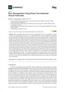
7. Visualization In this section, we investigate two visualization techniques that can broaden our understanding of the learned hierarchical features in SampleCNN. 7.1. Learned Filters Previous work in the music domain is limited to visualizing learned filters only on the first convolution layer [8,9,36] or visualizing responses after a filter is applied on a specific input [37,38]. The gradient ascent method has been proposed for directly seeing what is learned at a filter [39] and this technique has provided deeper understanding of what convolutional neural networks learn from images [40,41]. We applied the technique to our SampleCNN to observe how each filter in a layer processes the raw waveforms. The gradient ascent method is as follows. First, we generate random noise and back-propagate the errors in the network. The loss is set to the target filter activation. Then, we add the bottom gradients to the input with gradient normalization. By repeating this process several times, we can obtain the accumulated gradients-based waveform like signal at the input which is optimized to maximize the target filter activation. Examples of learned filters at each layer are in Figure 2. Although we can find the patterns that low-frequency filters are more visible along the layer, the estimated filters are still noisy. To show the patterns more clearly, we visualized them as spectrum in the frequency domain and sorted them by the frequency of the peak magnitude in Figure 3.
Appl. Sci. 2018, 8, 150
10 of 14
Figure 2. Examples of learned filters at each layer.
Layer 1
Layer 2
Layer 3
Layer 4
Layer 5
Layer 6
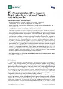
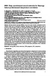
Figure 3. Spectrum of the estimated filters in the intermediate layers of SampleCNN which are sorted by the frequency of the peak magnitude. The x-axis represents the index of the filter, and the y-axis represents the frequency ranged from 0 to 11 kHz. The model used for visualization is 39 -SampleCNN with 59,049 samples as input. Visualization was performed using the gradient ascent method to obtain the accumulated gradient-based input waveform like signal that maximizes the activation of a filter in the layers. To effectively find the filter characteristics, we set the input size to 729 samples which is close to a typical frame size.
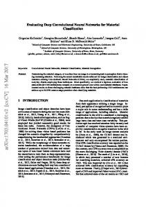
Note that we set the input waveform estimate to 729 samples in length because, if we initialize and back-propagate to the whole input size of the networks, the estimated filters will have large dimensions such as 59,049 samples in computing spectrum. Thus, the results are equivalent to spectra from a typical frame size. The layer 1 shows the three distinctive filter bands which are possible with the filter size with 3 samples (say, a DFT size of 3). The center frequency of the filter banks increases linearly in low frequency filter banks but, as the layer goes up, it progressively becomes steeper in high frequency filter banks. This nonlinearity was found in learned filters with a frame-level end-to-end learning [8] and also in perceptual pitch scales such as mel or bark. Finally, we visualized spectrum of the learned filter for each sampling rate up to 4th layers. In Figure 4, we can observe that all SampleCNN models focus (or zoom in) on the important low-frequency bands. We can also find that they show similar non-linear patterns to those in Figure 3.
Appl. Sci. 2018, 8, 150
Layer 1
11 of 14
Layer 2
Layer 3
2000 Hz
12000 Hz
4000 Hz
16000 Hz
8000 Hz
20000 Hz
Layer 4
Layer 1
Layer 2
Layer 3
Layer 4
Figure 4. Spectrum visualization of learned filters for different sampling rates. The x-axis represents the index of the filter, and the y-axis represents the frequency ranged from 0 to half the sampling rate. 3-sized filters are used for the first four modules in all models for fairly visualizing learned filters.
7.2. Song-Level Similarity Using t-SNE We extracted features from SampleCNN and aggregated them at different hierarchical levels of layer for each audio clip. We then embedded the song-level features into 2-D vectors using t-Distributed Stochastic Neighbor Embedding (t-SNE). Figure 5 visualizes the 2-D embedded features at different layer levels for selected tags to examine how multi-level feature aggregation technique enhances the performance. Songs with genre tag (Techno) are more closely clustered in the higher layer (−1 layer). On the other hand, songs with instrument tag (Piano) are more closely clustered in the lower layer (−3 layer). This may indicate that the optimal layer of feature representations can be different depending on the type of labels. Thus, combining different levels of features can improve the performance.
Techno
Piano
(a) -3 LAYER
(b) -1 LAYER
Figure 5. Feature visualization on songs with Piano tag and songs with Techno tag on MTAT using t-SNE. Features are extracted from (a) -3 LAYER and (b) -1 LAYER of the 39 -SampleCNN model pre-trained with MSD.
Appl. Sci. 2018, 8, 150
12 of 14
8. Conclusions In this article, we extend our previously proposed SampleCNN for music classification. Through the experiments, we found that downsampling music audio down to 8000 Hz does not significantly degrade performance but it saves training time. Second, transfer learning experiments with multi-level and multi-scale technique showed state-of-the-art results on most of the datasets we tested. Finally, we visualized the spectrum of the learned filters for each sampling rate and found that the SampleCNN model is actively focusing on (or zoom in on) important low-frequency bands. As future work, we will analyze why the sample-level architecture works well without input normalization and nonlinear function that compresses the amplitude, which are important when we use spectrogram as input. Also, we will investigate different filter visualization techniques to interpret the hierarchically-learned filters better. Acknowledgments: This research was supported by Basic Science Research Program through the National Research Foundation of Korea funded by the Ministry of Science, ICT & Future Planning (2015R1C1A1A02036962) and Korea Advanced Institute of Science and Technology (G04140049). Author Contributions: Jongpil Lee and Juhan Nam conceived and designed the experiments; Jongpil Lee and Jiyoung Park performed the experiments; Keunhyoung Luke Kim analyzed the data; Jongpil Lee and Juhan Nam wrote the paper. Conflicts of Interest: The authors declare no conflict of interest.
References 1.
2.
3.
4. 5.
6. 7.
8. 9.
10. 11.
Krizhevsky, A.; Sutskever, I.; Hinton, G.E. Imagenet classification with deep convolutional neural networks. In Proceedings of the 25th International Conference on Neural Information Processing Systems, Lake Tahoe, NV, USA, 3–6 December 2012; pp. 1097–1105. Mikolov, T.; Sutskever, I.; Chen, K.; Corrado, G.S.; Dean, J. Distributed representations of words and phrases and their compositionality. In Proceedings of the 26th International Conference on Neural Information Processing Systems, Lake Tahoe, NV, USA, 5–10 December 2013; pp. 3111–3119. Zhang, X.; Zhao, J.; Yann, L. Character-level convolutional networks for text classification. In Proceedings of the 28th International Conference on Neural Information Processing Systems, Montreal, QC, Canada, 7–12 December 2015; pp. 649–657. Kim, Y.; Jernite, Y.; Sontag, D.; Rush, A.M. Character-aware neural language models. arXiv 2016, arXiv:1508.06615. Sainath, T.N.; Weiss, R.J.; Senior, A.W.; Wilson, K.W.; Vinyals, O. Learning the speech front-end with raw waveform CLDNNs. In Proceedings of the 16th Annual Conference of the International Speech Communication Association, Dresden, Germany, 6–10 September 2015; pp. 1–5. Collobert, R.; Puhrsch, C.; Synnaeve, G. Wav2letter: An end-to-end convnet-based speech recognition system. arXiv 2016, arXiv:1609.03193. Zhu, Z.; Engel, J.H.; Hannun, A. Learning multiscale features directly from waveforms. In Proceedings of the Annual Conference of the International Speech Communication Association, San Francisco, CA, USA, 8–12 September 2016. Dieleman, S.; Schrauwen, B. End-to-end learning for music audio. In Proceedings of the IEEE International Conference on Acoustics, Speech and Signal Processing, Florence, Italy, 4–9 May 2014; pp. 6964–6968. Ardila, D.; Resnick, C.; Roberts, A.; Eck, D. Audio deepdream: optimizing raw audio with convolutional networks. In Proceedings of the International Society for Music Information Retrieval Conference, New York, NY, USA, 7–11 August 2016. Thickstun, J.; Harchaoui, Z.; Kakade, S. Learning features of music from scratch. arXiv 2017, arXiv:1611.09827. Dai, W.; Dai, C.; Qu, S.; Li, J.; Das, S. Very deep convolutional neural networks for raw waveforms. In Proceedings of the 2017 IEEE International Conference on Acoustics, Speech and Signal Processing, New Orleans, LA, USA, 5–9 March 2017; pp. 421–425.
Appl. Sci. 2018, 8, 150
12.
13.
14.
15. 16.
17.
18.
19.
20.
21.
22. 23. 24. 25.
26. 27.
28.
29.
30.
13 of 14
Aytar, Y.; Vondrick, C.; Torralba, A. Soundnet: Learning sound representations from unlabeled video. In Proceedings of the International Conference on Neural Information Processing Systems, Barcelona, Spain, 5–10 December 2016; pp. 892–900. Lee, J.; Park, J.; Kim, K.L.; Nam, J. Sample-level deep convolutional neural networks for music auto-tagging using raw waveforms. In Proceedings of the Sound Music Computing Conference (SMC), Espoo, Finland, 5–8 July 2017; pp. 220–226. Simonyan, K.; Zisserman, A. Very deep convolutional networks for large-scale image recognition. In Proceedings of the International Conference on Learning Representations, San Diego, CA, USA, 7–9 May 2015. Lee, J.; Nam, J. Multi-level and multi-scale feature aggregation using pre-trained convolutional neural networks for music auto-tagging. IEEE Signal Process. Lett. 2017, 24, 1208–1212. Tokozume, Y.; Harada, T. Learning environmental sounds with end-to-end convolutional neural network. In Proceedings of the IEEE 2017 IEEE International Conference on Acoustics, Speech and Signal Processing, New Orleans, LA, USA, 5–9 March 2017; pp. 2721–2725. Palaz, D.; Doss, M.M.; Collobert, R. Convolutional neural networks-based continuous speech recognition using raw speech signal. In Proceedings of the IEEE 2015 IEEE International Conference on Acoustics, Speech and Signal Processing, South Brisbane, Queensland, Australia, 19–24 April 2015; pp. 4295–4299. Palaz, D.; Collobert, R.; Magimai-Doss, M. Analysis of CNN-based speech recognition system using raw speech as input. In Proceedings of the 16th Annual Conference of the International Speech Communication Association, Dresden, Germany, 6–10 September 2015; pp. 11–15. Choi, K.; Fazekas, G.; Sandler, M. Automatic tagging using deep convolutional neural networks. In Proceedings of the 17th International Society of Music Information Retrieval Conference, New York, NY, USA, 7–11 August 2016; pp. 805–811. Choi, K.; Fazekas, G.; Sandler, M.; Cho, K. Convolutional recurrent neural networks for music classification. In Proceedings of the IEEE 2017 IEEE International Conference on Acoustics, Speech and Signal Processing, New Orleans, LA, USA, 5–9 March 2017; pp. 2392–2396. Pons, J.; Lidy, T.; Serra, X. Experimenting with musically motivated convolutional neural networks. In Proceedings of the IEEE International Workshop on Content-Based Multimedia Indexing (CBMI), Bucharest, Romania, 15–17 June 2016; pp. 1–6. Lee, J. Music Dataset Split. Available online: https://github.com/jongpillee/music_dataset_split (accessed on 22 January 2017). Tzanetakis, G.; Cook, P. Musical genre classification of audio signals. IEEE Trans. Speech Audio Process. 2002, 10, 293–302. Kereliuk, C.; Sturm, B.L.; Larsen, J. Deep learning and music adversaries. IEEE Trans. Multimed. 2015, 17, 2059–2071. Law, E.; West, K.; Mandel, M.I.; Bay, M.; Downie, J.S. Evaluation of algorithms using games: The case of music tagging. In Proceedings of the International Society for Music Information Retrieval Conference, Kobe, Japan, 26–30 October 2009; pp. 387–392. Schreiber, H. Improving genre annotations for the million song dataset. In Proceedings of the International Society for Music Information Retrieval Conference, Malaga, Spain, 26–30 October 2015; pp. 241–247. Bertin-Mahieux, T.; Ellis, D.P.; Whitman, B.; Lamere, P. The million song dataset. In Proceedings of the International Society for Music Information Retrieval Conference, Miami, FL, USA, 24–28 October 2011; Volume 2, pp. 591–596. Ioffe, S.; Szegedy, C. Batch normalization: Accelerating deep network training by reducing internal covariate shift. In Proceedings of the The 32nd International Conference on Machine Learning Lille, France, 6–11 July 2015. Dieleman, S.; Schrauwen, B. Multiscale approaches to music audio feature learning. In Proceedings of the International Society for Music Information Retrieval Conference, Curitiba, Brazil, 4–8 November 2013; pp. 116–121. Van Den Oord, A.; Dieleman, S.; Schrauwen, B. Transfer learning by supervised pre-training for audio-based music classification. In Proceedings of the International Society for Music Information Retrieval Conference, Taipei, Taiwan, 27–31 October 2014.
Appl. Sci. 2018, 8, 150
31. 32.
33.
34.
35. 36.
37.
38. 39. 40. 41.
14 of 14
Liu, J.Y.; Jeng, S.K.; Yang, Y.H. Applying topological persistence in convolutional neural network for music audio signals. arXiv 2016, arXiv:1608.07373. Güçlü, U.; Thielen, J.; Hanke, M.; van Gerven, M.; van Gerven, M.A. Brains on beats. In Proceedings of the International Conference on Neural Information Processing Systems, Barcelona, Spain, 5–10 December 2016; pp. 2101–2109. Pons, J.; Slizovskaia, O.; Gong, R.; Gómez, E.; Serra, X. Timbre analysis of music audio Signals with convolutional neural networks. In Proceedings of the 2017 25th European Signal Processing Conference, Kos Island, Greece, 28 August–2 September 2017. Jeong, I.Y.; Lee, K. Learning temporal features using a deep neural network and its application to music genre classification. In Proceedings of the International Society for Music Information Retrieval Conference, New York, NY, USA, 7–11 August 2016; pp. 434–440. Park, J.; Lee, J.; Park, J.; Ha, J.W.; Nam, J. Representation learning of music using artist labels. arXiv 2017, arXiv:1710.06648. Choi, K.; Fazekas, G.; Sandler, M.; Kim, J. Auralisation of deep convolutional neural networks: Listening to learned features. In Proceedings of the International Society for Music Information Retrieval Conference, Malaga, Spain, 26–30 October 2015, pp. 26–30. Bittner, R.M.; McFee, B.; Salamon, J.; Li, P.; Bello, J.P. Deep salience representations for f0 estimation in polyphonic music. In Proceedings of the International Society for Music Information Retrieval Conference, Suzhou, China, 23–28 October 2017. Choi, K.; Fazekas, G.; Sandler, M. Explaining deep convolutional neural networks on music classification. arXiv 2016, arXiv:1607.02444. Erhan, D.; Bengio, Y.; Courville, A.; Vincent, P. Visualizing Higher-Layer Features of a Deep Network; University of Montreal: Montreal, QC, Canada, 2009; Volume 1341, p. 3. Zeiler, M.D.; Fergus, R. Visualizing and Understanding Convolutional Networks; Springer: Berlin, Germany, 2014; pp. 818–833. Nguyen, A.; Yosinski, J.; Clune, J. Deep neural networks are easily fooled: High confidence predictions for unrecognizable images. In Proceedings of the Computer Vision and Pattern Recognition, Boston, MA, USA, 7–12 June 2015; pp. 427–436. c 2018 by the authors. Licensee MDPI, Basel, Switzerland. This article is an open access
article distributed under the terms and conditions of the Creative Commons Attribution (CC BY) license (http://creativecommons.org/licenses/by/4.0/).