The Journal of Neuroscience, June 10, 2015 • 35(23):8813– 8828 • 8813
Systems/Circuits
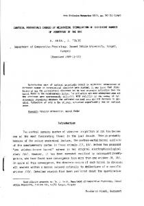
Endogenous Sequential Cortical Activity Evoked by Visual Stimuli Luis Carrillo-Reid, Jae-eun Kang Miller, Jordan P. Hamm, Jesse Jackson, and Rafael Yuste Neurotechnology Center, Department of Biological Sciences and Neuroscience, Columbia University, New York, New York 10027
Although the functional properties of individual neurons in primary visual cortex have been studied intensely, little is known about how neuronal groups could encode changing visual stimuli using temporal activity patterns. To explore this, we used in vivo two-photon calcium imaging to record the activity of neuronal populations in primary visual cortex of awake mice in the presence and absence of visual stimulation. Multidimensional analysis of the network activity allowed us to identify neuronal ensembles defined as groups of cells firing in synchrony. These synchronous groups of neurons were themselves activated in sequential temporal patterns, which repeated at much higher proportions than chance and were triggered by specific visual stimuli such as natural visual scenes. Interestingly, sequential patterns were also present in recordings of spontaneous activity without any sensory stimulation and were accompanied by precise firing sequences at the single-cell level. Moreover, intrinsic dynamics could be used to predict the occurrence of future neuronal ensembles. Our data demonstrate that visual stimuli recruit similar sequential patterns to the ones observed spontaneously, consistent with the hypothesis that already existing Hebbian cell assemblies firing in predefined temporal sequences could be the microcircuit substrate that encodes visual percepts changing in time. Key words: graph theory; in vivo calcium imaging; multidimensional population vectors; neuronal ensembles; primary visual cortex; two-photon microscopy
Introduction The coordinated activity of neurons firing in synchrony and organized in temporal sequences has been proposed as the generalized substrate for a wide variety of physiological computations and behaviors (Lorente de No, 1938; Hebb, 1949; Abeles, 1991; Seidemann et al., 1996; Baeg et al., 2003; Grinvald et al., 2003; Harris et al., 2003; Dragoi and Buzsa´ki, 2006; Fujisawa et al., 2008; Pastalkova et al., 2008; Buzsa´ki, 2010; Crowe et al., 2010; Dragoi and Tonegawa, 2011; Harvey et al., 2012). However, little is known about how sequential activity patterns are generated and whether they have a functional significance. For example, it has been proposed that specific groups of neurons firing in sequences could represent canonical microcircuit motifs (Hebbian cell assemblies) that can be recalled reliably (Hebb, 1949; Huyck,
Received Dec. 22, 2014; revised May 5, 2015; accepted May 6, 2015. Author contributions: L.C.-R., J.K.M., and R.Y. designed research; J.K.M. performed research; L.C.-R., J.K.M., J.P.H., and J.J. analyzed data; L.C.-R. and R.Y. wrote the paper. This work was supported by the National Eye Institute–National Institutes of Health (Grants DP1EY024503, R01EY011787, and F32EY022579) and the Defense Advanced Research Projects Agency–Department of Defense (Contract W91NF-14 –1-0269). This material is based upon work supported by, or in part by, the U.S. Army Research Laboratory and the U.S. Army Research Office (Contract W911NF-12–1-0594, MURI). We thank Inbal Ayzenshtat for doublet analysis and laboratory members for valuable comments. The authors declare no competing financial interests. This article is freely available online through the J Neurosci Author Open Choice option. Correspondence should be addressed to Luis Carrillo-Reid, PhD, Department of Biological Sciences, Columbia University, 902 NWC Building 550 West 120 Street, Box 4822, New York, NY 10027. E-mail:
[email protected]. DOI:10.1523/JNEUROSCI.5214-14.2015 Copyright © 2015 Carrillo-Reid et al. This is an Open Access article distributed under the terms of the Creative Commons Attribution License Creative Commons Attribution 4.0 International, whichpermitsunrestricteduse,distributionandreproductioninany medium provided that the original work is properly attributed.
2001; Harris, 2005; Lansner, 2009), allowing the formation of complex representations from basic multicellular functional units (Luczak et al., 2009). Moreover, Hebb’s cell assembly hypothesis postulates that neurons firing in sequential order will create activity cycles reverberating in the absence of external stimulation (Hebb, 1949). Accordingly, there is in vitro and in vivo evidence that the visual cortex can generate repeated patterns of spontaneous activity that resemble those observed under visual stimulation (Kenet et al., 2003; MacLean et al., 2005; MacLean et al., 2006; Miller et al., 2014). In addition, visual cortical neurons responding to the same orientation display similar spontaneous activity (Ch’ng and Reid, 2010) and have a higher probability to be connected among themselves (Ko et al., 2011), suggesting that synaptic plasticity, perhaps following Hebbian learning rules, could explain repeated temporal dynamics. Using two-photon calcium imaging with single-cell resolution in vivo, we recently found that most cortical activity occurred in the form of coactive groups of cells defining neuronal ensembles (Miller et al., 2014). Although the same ensembles were repeatedly triggered by visual stimuli of the same orientation, these repetitions were never exact and neurons could promiscuously join different ensembles. Interestingly, the same ensembles that were visually evoked could be detected in the spontaneous activity, suggesting that cortical circuits may build a response to sensory stimuli using internal building blocks. Although that recent work described the spatial structure of neuronal ensembles, it did not examine whether recurrent temporal patterns were also present. To further understand the temporal structure and properties of neuronal ensembles, we have now used independent analytical tools that capture spatiotempo-
Carrillo-Reid et al. • Temporally Structured Cortical Dynamics
8814 • J. Neurosci., June 10, 2015 • 35(23):8813– 8828
ral population dynamics (Carrillo-Reid et al., 2011) and applied it to the same dataset (Miller et al., 2014). As before, our approach allowed us to identify groups of neurons firing in synchrony that reliably represent specific visual scenes. However, in addition, we find that these ensembles of neurons from primary visual cortex encode natural stimuli with temporally structured network dynamics. Sequential activity patterns that emerge in the absence of visual stimulation are also recruited by recurrent natural scenes, demonstrating repeated temporally structured network activity in primary visual cortex of awake mice. Our results indicate that the representation of visual percepts could be implemented using endogenous spatiotemporal dynamics of neural circuits.
Materials and Methods Note on present study This study represents an independent analysis of experiments described previously (Miller et al., 2014). Although the raw data are mainly the same, the questions investigated and analytical tools are different, focusing on the detection and characterization of temporal patterns.
Animal surgery All animal procedures were performed according to the guidelines of Columbia University Institutional Animal Care Guidelines and have been described previously (Miller et al., 2014). Briefly, experiments were performed on C57BL/6 male mice (n ⫽ 4) or on parvalbumin-Cre (n ⫽ 1) or somatostatin-Cre (n ⫽ 2) ⫻ LSL-tdTomato transgenic male mice obtained from The Jackson Laboratory at the age of postnatal day 40 – 80. Mice were anesthetized with isoflurane (1–2%). A titanium head plate was attached to the skull using dental cement. The site for craniotomy was delimited using a dental drill over left V1. To facilitate head fixation, mice underwent training to maneuver on a spherical treadmill for 1–3 h for 2–3 d.
Functional multicell calcium imaging On the imaging day, the part of the skull marked previously was removed while mice were anesthetized with isoflurane. Bulk loading was performed using the calcium indicator Oregon Green BAPTA-1 AM (Invitrogen) dissolved in 4 l of DMSO plus 20% Pluronic F-127 (Invitrogen) and diluted with 35 l of pipette solution (150 mM NaCl, 2.5 mM KCl, 10 mM HEPES, pH 7.4). Sulforhodamine 101 (Invitrogen) was added to the solution pipette to label astrocytes. Pipette solution was injected in layer 2/3 of V1 under visual control (10 p.s.i., 8 min per site) in 3 different locations. Cortical neurons were monitored with a two-photon microscope (Moveable Objective Microscope; Sutter Instruments) attached to a Ti: sapphire laser (Chameleon Vision II; Coherent) with 880 nm excitation light focused through a 20⫻ [0.95 numerical aperture (NA); Olympus] or 25⫻ (1.05 NA; Olympus) water-immersion objective. Scanning and image acquisition were controlled by the Sutter Instruments software Mscan. The optical field recorded was ⬃315 ⫻ 315 m. Short videos (⬃720 s) with a sample rate of 125–250 ms/frame were collected at time intervals of 5–10 min for up to 2 h.
Visual stimulation Visual stimuli were generated using MATLAB (The MathWorks) Psychophysics Toolbox and displayed on a LCD monitor positioned 15 cm from the right eye at 45° to the long axis of the animal. Spontaneous activity in layer 2/3 of visual cortex was recorded under complete darkness in an optically isolated laser room at the beginning of the experiments and sometimes in the middle of the experiments (with a monitor and room lights turned off). The imaging setup and the objective were completely enclosed with blackout fabric and a black electrical tape and there was no detectable light coming into the mouse eye during the spontaneous condition. Visual stimuli consisted of full-field drifting gratings or natural scenes. Sine or square-wave gratings (100% contrast, 0.035 cycles/degree, 2 cycles/s) drifting in 8 different directions randomly were presented for 5 s, followed by 5 s of mean luminescence. Natural scenes consisted of 10 distinct natural scenes displayed repeatedly for 30 s
using the MATLAB Psychophysics Toolbox synchronized with image acquisition.
Image processing Image processing was performed with ImageJ version 1.42q software and custom-made programs written in MATLAB as described previously (Mao et al., 2001; Cossart et al., 2003; Carrillo-Reid et al., 2008). Acquired images were processed to correct motion artifacts (Dombeck et al., 2007; Evangelidis and Psarakis, 2008; Kaifosh et al., 2013). Active neurons were automatically identified, coordinates for each cell in a 2D plane were assigned, and the calcium transients were measured as a function of time. Calcium transients were computed as changes in fluorescence: (Fi ⫺ F0)/F0, where Fi denotes the fluorescence intensity at any frame and F0 denotes the basal fluorescence of each neuron (Miller et al., 2014). Spike probability was inferred from calcium signals using a fast, non-negative deconvolution method (Vogelstein et al., 2010) and then a threshold of 3 SDs above noise was determined from spike probabilities of the entire population in each experiment. The spike onsets inferred from calcium signals were used to represent the activity of the network. We constructed an N ⫻ F binary matrix, where N denotes the number of active neurons and F represents the total number of frames for each video. For the analysis, only calcium transients elicited by neurons were considered. Each row in the binary matrix represents the activity of one neuron. To visualize all of the active neurons, the binary matrix was plotted as a raster plot in which ones are represented by dots. The time histogram of the raster plot illustrates the overall behavior of the network (Mao et al., 2001; Cossart et al., 2003; Carrillo-Reid et al., 2008).
Analytical tools Vectorization of the network activity. To identify neuronal pools firing in synchrony, temporal vectors were constructed that represent the simultaneous activation of different neurons. We tested the significance of the peaks of synchrony that we observed against the null hypothesis that the synchronous firing of neuronal pools is given by a random process (Shmiel et al., 2005, 2006). We generated 1000 shuffled raster plots (see “Reshuffling methods” section below) and compared the distribution of the random peaks against the peaks of synchrony observed in the real data (Mao et al., 2001; Cossart et al., 2003; Carrillo-Reid et al., 2008). Peaks of synchrony are defined by all of the adjacent high-activity frames in a given time window (Carrillo-Reid et al., 2008). Only the peaks of synchrony with more than the cells expected by chance ( p ⬍ 0.01) were considered for further analysis. Synchronously active neuronal pools define population vectors representing the overall activity of the network. Such vectors can be used to describe the network activity as a function of time (Schreiber et al., 2003; Stopfer et al., 2003; Brown et al., 2005; Sasaki et al., 2007; Carrillo-Reid et al., 2008). The population vectors representing the network activity define a multidimensional space in which the number of dimensions is given by the total number of active cells in high-activity frames. It has been shown that the temporal vectorization of the network activity allows the discrimination of similar patterns repeated at different times (Schreiber et al., 2003; Ikegaya et al., 2004; Brown et al., 2005; Carrillo-Reid et al., 2008). Term frequency–inverse document frequency normalization. After the identification of the vectors with low probability to be random events ( p ⬍ 0.01), we normalized the [N ⫻ T] binary matrix (where N ⫽ number of active cells and T ⫽ the number of significant vectors) that represents the activity of the network. The normalization was based on a classic term frequency (TF)–inverse document frequency (IDF) search algorithm widely used in the field of natural language processing to recognize words that are key to relevant documents (Lan et al., 2009; Lu et al., 2009; Islamaj Dog˘an and Lu, 2010; Garbarine et al., 2011). The main purpose of the normalization is to find the neurons that are more relevant to specific visual stimuli. The TF–IDF matrix elements are given by TF*IDF for each active neuron at each significant frame. TF measures active neurons normalized by the total number of active neurons for each frame. However, cells that are frequently active have little effect in defining neuronal ensembles even though they can be key players orchestrating the transitions between different groups (Carrillo-Reid et al., 2008). Therefore, to reduce the impact of highly active neurons in the definition
Carrillo-Reid et al. • Temporally Structured Cortical Dynamics
of a neuronal ensemble, we computed IDF, which measures the number of times that a neuron appears in the total number of significant vectors. For this particular case, IDF was defined as follows: IDF(i) ⫽ log(total vectors/vectors(i)), where vectors(i) denote all of the significant vectors where neuron i appears. TF–IDF captures how important a word is in a collection of documents. In the context of the present work, TF–IDF defines the importance of a specific neuron in a collection of significant vectors that represent neuronal ensembles. Representation of multidimensional datasets in time. To construct similarity maps, all of the possible vector pairs taken from the normalized TF–IDF matrix were compared. The similarity index between a pair of vectors is defined by their normalized inner product (Schreiber et al., 2003; Sasaki et al., 2007; Carrillo-Reid et al., 2008; Carrillo-Reid et al., 2009) as follows: cos() ⫽ A 䡠 B /兩兩A兩兩 兩兩B兩兩, which represents the cosine of the angle between two vectors. If two population vectors in an “n” dimensional space point in the same direction, the similarity index has a value of 1. In neural network context, high similarity values between two different time points describe repeated groups of neurons firing in synchrony. The inner product between different elements of a multidimensional space normalized by the magnitude of the elements has been widely used in search engines because it represents a computationally efficient algorithm that captures the similarities between documents. The visualization of the angles between all of the possible vector pairs represents a multidimensional reduction from “n” dimensions mapped into a 3D space, where the first two dimensions denote the significant vectors as a function of time and the third dimension indicates the angle between them. Significant patterns can be identified by vectors denoted by repetitive structures in the similarity maps (Victor and Purpura, 1996; Levy et al., 2001; Schreiber et al., 2003; Morelli et al., 2006; Kreuz et al., 2007; Carrillo-Reid et al., 2008; Tiesinga et al., 2008). To determine whether similar patterns of activity repeated in a statistically significant manner, we shuffled the normalized TF–IDF matrix, preserving the dimensionality of population vectors, and compared the probability distribution of similarity coefficients from real data and shuffled data. Identification of neuronal ensembles. To detect different groups from multidimensional datasets, the cosine similarity of all possible vector pairs was used. Defined structures in the similarity maps (independent of the distance function chosen) have been widely used to detect recurrent patterns (Victor and Purpura, 1996; Levy et al., 2001; Schreiber et al., 2003; Morelli et al., 2006; Kreuz et al., 2007; Tiesinga et al., 2008). However, in those approaches, the independent variable considered to perform the computations was given by the identity of single neurons. Similarity maps generated by vectors in which dimensionality is defined by individual trials give valuable information about neuronal correlations, but cannot capture directly the sequential activity patterns that define a network. The main difference with our approach is that we consider the number of active cells as the dimension of the vectors, so our similarity maps can reveal temporal patterns (Sasaki et al., 2007; CarrilloReid et al., 2008; Carrillo-Reid et al., 2009; Carrillo-Reid et al., 2011). Neuronal ensembles are defined by a subset of neurons that reocurr at different times. To highlight significant patterns from similarity maps, we transform them in a binary matrix M of size (T ⫻ T ). The cutoff value represents the percentage of total cells that are coactive in two different frames above chance levels. A neuronal ensemble is defined by groups of neurons with synchronous, recurrent, and alternate activity (Hebb, 1949; Carrillo-Reid et al., 2008; Carrillo-Reid et al., 2009; Carrillo-Reid et al., 2011). To identify neuronal ensembles, we obtained the singular value decomposition (SVD) of the significant patterns matrix. SVD has been widely used in signal processing analysis because it allows the identification of components representing the main features of a given system. Formally, the SVD of a real matrix can be expressed as the multiplication of three factors, U, 冱, and V T, where U and V T represent orthonormal bases and the elements of 冱 are the singular values. In our particular case, the matrix M, which contains the information of the significant patterns of activity, is a real symmetric matrix; so V ⫽ U. Therefore, the SVD is given by M ⫽ V 冱 V T. The number of singular values that defines the total number of neuronal ensembles was determined by the rate of singular values decaying above chance levels. Rapid decaying singular values can reproduce original data with high accuracy. SVD is a method to
J. Neurosci., June 10, 2015 • 35(23):8813– 8828 • 8815
factorize a dataset into linearly independent components that in this case represent neuronal ensembles. Analogous results were obtained with similar approaches such as locally linear embedding and clustering analysis (Carrillo-Reid et al., 2011). However, the main advantage of using SVD is the unsupervised identification of neuronal ensembles without the necessity to define a specific number of clusters; this fact is crucial to identify the most representative cells during the course of an experiment, opening the possibility to manipulate ad libitum identified neurons with single-cell resolution. Identification of closed cycles with graph theory. After the identification of the neuronal ensembles, we looked for closed trajectories in the sequential activity patterns that are a characteristic of Hebbian cell assemblies (Hebb, 1949; Harris, 2005; Carrillo-Reid et al., 2009). Neuronal ensembles transitions were plotted as a function of time (Lee and Wilson, 2002; Carrillo-Reid et al., 2009; Carrillo-Reid et al., 2011). From these transitions, we constructed isomorphic directed graphs with the properties of Hamiltonian or Eulerian cycles. To define sequential patterns mathematically that occur above chance levels, we just considered Hamiltonian or Eulerian closed cycles. The number of closed cycles that occurred in spontaneous activity or visually evoked activity was significantly different compared with the number of closed cycles from shuffled data. A Hamiltonian cycle of a directed graph (digraph) is a closed trajectory that contains every vertex of the graph exactly once. An Euler cycle is a closed trajectory passing through every edge exactly once (Diestel, 2005). Digraphs, represented by adjacency matrices, allow the automatic identification of template sequences. Template sequences indicate repetitive transitions between neuronal ensembles and are useful to identify spatiotemporal patterns with high probability of recurrence. The use of graph theory applied to neuronal ensembles transitions revealed that complex cycles of activity can be composed by smaller cycles or “primitives” that could represent basic procedures (Hebb, 1949; Bienenstock and Geman, 1995; Hammer, 2003; Abeles et al., 2004; Carrillo-Reid et al., 2009). Cross-correlation analysis. We performed the normalized crosscorrelation between all of the possible combinations of neurons that belong to the same neuronal ensemble and between all of the combinations of neurons belonging to neuronal ensembles firing in sequence repeatedly. Note that, because of the multidimensional nature of the network activity, it is extremely difficult and time consuming to define neuronal ensembles from an exhaustive cross-correlation of all possible neuron pairs (Carrillo-Reid et al., 2008; Carrillo-Reid et al., 2011). Cells belonging to the same neuronal ensemble present high cross-correlation values at zero time lag, whereas neurons from two sequential neuronal ensembles have high cross-correlation values at specific time lags that reflect the temporal structure between two defined groups. Granger causality. To determine whether the occurrence of a given neuronal ensemble “causes” the emergence of another neuronal ensemble, we performed a Granger causality test (Granger, 1969) between the activation time courses of all possible combinations of neuronal ensembles. Although causality per se is a philosophical concept, the Granger approach infers a practical version of causality by assessing the degree to which time course “b” can predict time course “a” better than time course “a” alone. We estimated the activation time course for each neuronal ensemble based on the similarity index function of the most representative cells. We then performed a multiple regression of each ensemble onto several time-shifted versions of itself to obtain R 2 and then calculated the change in R 2 after adding time-shifted versions of other ensemble activation time courses (termed herein “Granger coefficients”). Granger coefficients reflected R 2 change in the time course of ensemble “a” gained by considering the back-shifted time course of another ensemble “b” in addition to the back-shifted time course “a.” To discard nonzero Granger coefficients that could be occurring by chance, we shuffled the time courses of each ensemble 1000 times, calculating the random distribution for each shuffle separately for each experimental condition. Doublets analysis. To identify sequential pairs of neurons with fixed time intervals, we performed an exhaustive matching algorithm that searches for a given time interval in all of the possible combinations of active neurons (Ayzenshtat et al., 2010). We consider as events only
Carrillo-Reid et al. • Temporally Structured Cortical Dynamics
8816 • J. Neurosci., June 10, 2015 • 35(23):8813– 8828
A
B
C
D
E
Figure 1. Two-photon imaging of population activity in primary visual cortex of freely moving animals. A, Experimental setup. Mice are head fixed to the stage of a two-photon microscope on top of a foam ball floating in air that allows them to move freely. A monitor placed 15 cm contralateral to the craniotomy site displays different visual stimuli that are computer controlled and consist of drifting gratings of four orientations moving in two different directions, nonstimulus or natural scenes. For simplicity, orientation bars are represented by lines and not the actual patterns presented. B, Visual cortical neurons bulk loaded with Oregon green showing the average of 1000 consecutive frames. White dots indicate individual cells. Red circles indicate neurons shown in C. Scale bar, 50 m. C, Calcium transients recorded from the cells shown in B. Cortical neurons have episodes of spontaneous activity. D, Spike detection of the calcium transients taken from the insert in C. Lines on bottom (spikes) indicate neuronal activity. Dashed line indicates a threshold ⬎3 times the SD of noise. Spikes were used to construct binary arrays representing the activity of each neuron. E, Raster plot representing the overall activity of the network in different experimental conditions is shown at the top. Each row represents an active neuron. Temporal histogram of the spontaneous activity observed in cortical neurons is shown at the bottom. Dashed line indicates a threshold value used to select the synchrony peaks with a low probability ( p ⬍ 0.01) of being random. Note the presence of spontaneous periods of synchronous activity without apparent periodicity.
doublets that are present above chance levels compared with the network activity shuffled in time or in space. Doublet analysis emphasizes the existence of pairs of neurons with structured temporal activity. Reshuffling methods. We performed four different spatiotemporal shuffling paradigms of our datasets, each catered specifically to a point of interest to robustly assess statistical significance in the absence of obvious parametric test for population analysis. These approaches involved shuffling 1000 times the binary matrices representing the overall activity of the network and/or ensemble activation time courses as follows: (1) preserving the interburst intervals but shuffling their orders across time within cells (used to identify the maximum number of cells coactive by chance), (2) preserving the activity within time frames but shuffling the events across cells (used to establish the stability and robustness of ensembles while maintaining the dimensionality of the population vectors), (3) preserving the temporal relationships between cells but shuffling the nature and direction of their sequences by swapping spikes at the pairwise-level, and (4) randomly time shifting the activity within each cell (used for assessing the significance of Granger coefficients by holding autocorrelations constant within cells).
Results Detecting neuronal coactivations in mouse visual cortex To measure neuronal responses to visual stimulation in neuronal populations, we performed in vivo two-photon calcium imaging from layer 2/3 of primary visual cortex from awake, freely moving mice (Fig. 1A) because calcium imaging allows the spatial and
temporal study of neural networks with single-cell resolution (Yuste and Katz, 1991; Ohki et al., 2005; Grewe and Helmchen, 2009; Wallace and Kerr, 2010). For each experiment, the imaged field of view was ⬃315 ⫻ 315 m, containing on average 80 ⫾ 25 active neurons (Fig. 1B; n ⫽ 7 mice). For analysis, we assigned 2D spatial regions of interest to each cell in the field of view and measured their calcium transients as a function of time (Fig. 1C). To identify action potential activity represented by calcium transients, we estimated the spike probability as described previously (Vogelstein et al., 2010) (Fig. 1D) and considered for analysis only those signals above a threshold ⬎3 times SDs from the background fluorescence noise (Mao et al., 2001; Cossart et al., 2003; Carrillo-Reid et al., 2008). These suprathreshold signals were used to generate binary arrays that depict population activity as raster plots (Fig. 1E), where each row represents an active neuron and each column in the raster plot signals the overall activity of the network at a specific time. In these raster plots, neuronal activity was widely distributed across the entire population of imaged cells (Fig. 1E). Moreover, the time histogram of population activity (Fig. 1E, bottom) showed the prevalence of periods of synchronous firing in cortical neurons under both spontaneous and visually evoked activity, as shown previously (Miller et al., 2014). These spontaneous peaks of synchrony did not show apparent periodicity and occurred at variable time intervals (76 ⫾ 35 synchronous epochs
Carrillo-Reid et al. • Temporally Structured Cortical Dynamics
A
B
J. Neurosci., June 10, 2015 • 35(23):8813– 8828 • 8817
repeat above chance levels, which is consistent with our past work (Miller et al., 2014).
Identification of neuronal groups activated by visual stimuli Even though responses to visual stimuli of layer 2/3 neurons in primary visual cortex have been widely characterized in many experimental conditions (Victor and Purpura, 1996; Tiesinga et al., 2008; Sawinski et al., 2009; Kampa et al., 2011; Marshel et al., 2011; Espinosa and Stryker, 2012; Gavornik and Bear, 2014), the identification C D of neuronal groups during the course of an experiment in which coordinated activity represents specific visual percepts remains unexplored because optical or electrical techniques that provide largescale multineuronal data are still relatively recent. To identify groups of neurons that respond to a given orientation repeatedly, we used drifting gratings at four different orientations and two opposite directions. Drifting gratings were presented randomly intermixed with interstimulus inFigure 2. Representation of network activity as multidimensional arrays. A, Schematic representation of network activity tervals of the same duration (Fig. 3A), as vectorization. Each vector represents a group of neurons firing in synchrony at a given time point. Cells active at different times (t1, t2, tn) are highlighted in red (left). Each frame is represented as a binary vector of “n” dimensions. The dimensionality of the vectors described previously (Miller et al., 2014). is given by the total number of active cells in a specific field of view (80 ⫾ 25 neurons; n ⫽ 7 mice). B, TF–IDF normalization was Visual responses to drifting gratings calculated to decrease the overall weight of neurons with high activity (red marks). C, Schematic representation of cosine similarity evoked peaks of synchronous activity reused to define repeated activity patterns. D, Probability distribution of similarity coefficients from all possible vector pairs between flecting the overall behavior of the netthree different experimental conditions. Shaded area denotes not significant values ( p ⬎ 0.05) for a range of similarity coeffi- work (Fig. 3A, bottom). cients. For similarity coefficients ⬎0.24, real data are significantly different from shuffled data. Because individual cells can respond to multiple orientations (Victor and Purpura, 1996; Mrsic-Flogel et al., 2007; per 300 s, each epoch comprises 6 ⫾ 3 active frames; n ⫽ 7 mice). Marshel et al., 2011; Espinosa and Stryker, 2012), it is difficult to Only peaks of synchronous activity with negligible probability of identify a representative group of neurons that respond to speoccurring by chance were considered for further analysis (Fig. 1E; cific visual stimuli (Kampa et al., 2011). To find neuronal ensemp ⬍ 0.01; see Materials and Methods). bles responding reliably to a given visual stimulus, we analyzed the network activity as a whole using population vectors because Multidimensional vectors depict repeated activity patterns vectorization allows rigorous and quantitative comparison of acRaster plots can be understood as multidimensional arrays where tivity patterns at different times (Schreiber et al., 2003; Brown et al., 2005; Sasaki et al., 2007; Carrillo-Reid et al., 2008). To detect each point in time defines a population vector (Fig. 2A) the dimensionality of which corresponds to the total number of active repeated patterns of activity, we constructed similarity maps of cells (Stopfer et al., 2003; Brown et al., 2005; Sasaki et al., 2007; the normalized inner product of all possible vector pairs. SimiCarrillo-Reid et al., 2008). Because cells with high activity levels larity maps still reflect the temporal characteristics of the network can bias the identification of groups of neurons responding to activity and can be used to visualize similar population vectors specific visual stimuli, we performed TF–IDF of the binary arrays occurring at specific time points (Sasaki et al., 2007; Carrillo-Reid et al., 2008; Carrillo-Reid et al., 2009; Carrillo-Reid et al., 2011). (Fig. 2B). TF–IDF has been used widely in search engines to lower the weight of frequent terms. In the context of neural activity, Significant patterns obtained from these similarity maps repreword vectors represent the activity of each cell and document sent the existence of stable structures in the responses (Victor and Purpura, 1996; Levy et al., 2001; Schreiber et al., 2003; Morelli et vectors represent a population vector (Fig. 2B). To detect repetitions from population vectors above chance al., 2006; Kreuz et al., 2007; Tiesinga et al., 2008) that occurred above chance levels (Fig. 2D) and can be used to identify the time levels, we computed the similarity coefficients (Fig. 2C) of the normalized TF–IDF matrix from all of the possible combinations when similar population vectors were present (Fig. 3B). The maof vectors among different experimental conditions and comtrix of significant patterns can be factorized by SVD in the three pared them with the similarity coefficients obtained from shuffactors, U, 冱, and V T. The strongest singular values that define the total number of neuronal ensembles were determined by the fled data preserving the activity within time frames (Fig. 2D). Similarity coefficients above chance levels demonstrated that rate of singular values decaying above chance levels (Fig. 3C). On average, for the experimental condition of drifting gratings, we similar population vectors occurred in spontaneous and visually identified 6 ⫾ 1 ensembles (Fig. 3C; n ⫽ 7 animals) representing evoked activity. These experiments demonstrated that populathe factors that can reproduce the main features of the original tion vectors defining network activity in primary visual cortex
Carrillo-Reid et al. • Temporally Structured Cortical Dynamics
8818 • J. Neurosci., June 10, 2015 • 35(23):8813– 8828
A
C
B
D
E
H
G
F
I
J
K
Figure 3. Neuronal ensembles define recurrent groups of neurons responding to specific visual stimuli. A, Raster plot of network activity responses to drifting gratings (top). Each row represents an active neuron. Gray stripes indicate the duration of the stimuli. Temporal histogram represents the number of coactive cells over time (middle). Dashed line indicates a threshold value used to select the synchrony peaks with low probability ( p ⬍ 0.01) of being random events. Note that peaks of synchronous activity can be observed also in the absence of visual stimulation. Four different orientations and two directions were presented randomly (bottom). B, Binary matrix extracted from similarity map representing significant patterns of activity factorized by SVD. Black patterns indicate recurrent coactive cells at different moments. C, Magnitude of singular values used to determine the number of neuronal ensembles. Red line indicates 2⫻ the magnitude of singular values from shuffled data. Cutoff value indicates the most representative number of neuronal ensembles corresponding to a significant change in slope of the magnitude of contiguous singular values. Networks of 80 ⫾ 25 neurons stimulated with four drifting gratings can be defined by 6 ⫾ 1 neuronal ensembles (n ⫽ 7 mice). D, First six factors of SVD that reproduce reliably the overall behavior of the network. Bars on top indicate orientations; empty squares represent recurrent neuronal ensembles appearing in the absence of visual stimuli. E, Neuronal ensembles sorted in time defined by the most representative factors of singular value decomposition. Each row represents a neuronal ensemble. Note that some neuronal ensembles occurred spontaneously in the absence of visual stimulation (empty squares). A neuronal ensemble represents a group of cells with synchronous, recurrent, and alternating activity. F, Calcium transients from five of the most representative cells that defined neuronal ensemble 1 (blue; 90 degrees orientation). Blue stripes represent visual stimuli with 90 degrees orientation. Some cells responded to only one orientation and others responded to multiple orientations. Colors on bottom depict different orientations. Note that neuronal ensembles entrained by drifting gratings represent neurons with synchronous and recurring activity imposed by visual stimuli. G, Similarity function of the most representative neurons (core) responding to 90 degrees orientation (top). A threshold of 3 times the SD of the noise indicates when a specific neuronal ensemble matches a given drifting grating (blue). The percentage of matches demonstrates that core ensembles can predict when a given visual stimuli was presented (bottom; p ⬍ 0.0001; Mann–Whitney test). H, Spatial maps of the neurons belonging to different neuronal ensembles. Black cells show the most representative neurons of each ensemble (core) that can reproduce the overall behavior of the network. Scale bar, 50 m. I, Center of mass from different ensembles (left) and the mean distance between all of the neurons from each ensemble (right) demonstrate that ensembles are anatomically widespread. J, Percentage of coactive cells between ensembles and core ensembles ( p ⫽ 0.0001; Mann–Whitney test). K, Orientation selectivity index from neurons belonging to ensembles or cores ( p ⫽ 0.3095; Mann–Whitney test). Note that cells with broad tuning can be part of core ensembles.
Carrillo-Reid et al. • Temporally Structured Cortical Dynamics
data. Each factor from SVD depicts repetitive features of a multidimensional array that in our case represents the time when a specific orientation was presented (Fig. 3D). Repeated coactive patterns were readily observable and corresponded to distinctive orientation gratings (Fig. 3E), which is consistent with our previous work (Miller et al., 2014). Although our analytical tools allowed us to define neuronal ensembles that distinguished specific orientations accurately, we could not separate between opposite directions at the population level, consistent with the fact that direction selectivity of individual neurons in V1 is lower than orientation selectivity (Marshel et al., 2011). These results confirmed the existence of neuronal ensembles in primary visual cortex that respond to a given orientation and further extend our previous work (Miller et al., 2014) identifying automatically the time when a given ensemble occurs. Cells with diverse orientation selectivity compose neuronal ensembles To study the relation between neuronal ensembles and orientation selectivity, a known functional property of the mammalian primary visual cortex (Hubel and Wiesel, 1959), population responses to visual stimuli were studied. We identified the most representative neurons of each neuronal ensemble (base elements or core neurons) using a classic search engine algorithm to recognize words that are key to documents (Fig. 2; see Materials and Methods). In the context of population dynamics, each neuron represents a word and documents define the collection of high-dimensional vectors comprising each group. Calcium transients from neurons belonging to a given ensemble showed that neuronal ensembles could be composed of cells that just responded to a given orientation and of cells responding to multiple orientations (Fig. 3F ). Base elements (core neurons) consisted of groups of 14 ⫾ 5 cells (n ⫽ 7 animals) and reproduced the overall network behavior (Fig. 3G). Ensembles did not simply reflect spatial clusters (Fig. 3H ) because the centroid of cells belonging to each ensemble was located in the middle of the optical field (Fig. 3I, left) and the mean distance between all of the neurons from each ensemble covered most of the recorded area (Fig. 3I, right). This altogether confirmed a “salt and pepper’ anatomical distribution of neurons (Espinosa and Stryker, 2012) despite highly tuned visual responses. Cells belonging to core ensembles had low overlap (Fig. 3J ), indicating the possibility to manipulate identified subnetworks with single-cell resolution to drive behavioral outcomes. Interestingly, even if core ensembles were very selective for a given orientation, they could still have neurons with low orientation selectivity (Fig. 3K ). Our analysis thus demonstrated that specific assortments of neurons reliably respond to a given visual stimuli as a group, a first step to studying the temporal characteristics of neuronal ensembles. Natural scenes trigger sequences of neuronal ensembles We then turned our attention to the temporal analysis of the dynamics between neuronal ensembles using natural scenes as visual stimulus. Sequential activity patterns between neuronal groups have been proposed as associated cells that can act as a temporally closed system after sensory stimulation has ceased, constituting the implementation of a mental representation (Hebb, 1949). To identify repetitive sequential patterns between neuronal ensembles, we created an artificial experimental paradigm in which we presented 10 different natural scenes for 30 s repeated in the same sequential order many times. This enabled us to be certain that the transitions observed were evoked by our
J. Neurosci., June 10, 2015 • 35(23):8813– 8828 • 8819
visual stimuli and not by external factors independent of visual stimulation. The expectation was to find closed cycles of activity between neuronal ensembles that were precisely related to recurrent stimuli repeated many times. To describe sequential activity patterns from cortical networks in vivo, we applied graph theory techniques to the temporal transitions between neuronal ensembles identifying template pathways embedded in closed cycles (Fig. 4A; see Materials and Methods). For this analysis, we just considered Hamiltonian or Eulerian closed cycles that are represented by unique adjacency matrixes (Fig. 4B; see Materials and Methods) and allow the identification of recurrent transitions between neuronal ensembles (Carrillo-Reid et al., 2009; CarrilloReid et al., 2011). Closed cycles have unique mathematical properties that allow their identification from a sequence of events. It is important to highlight that each transition implies specific groups of neurons firing in synchrony and recurrently above chance levels determined from shuffled data. To investigate whether closed cycles between neuronal ensembles in our experiments occurred above chance levels, we used a conservative approach. We shuffled the transitions describing a given experiment and compared the total number of Hamiltonian or Eulerian closed cycles that appeared in real data with the total number of closed cycles that can emerge by chance in spontaneous and visually evoked conditions. Indeed, closed cycles describing our experiments were significantly different from closed cycles emerging by chance (Fig. 4C). Moreover, the same closed cycles that appeared in real data were never found in shuffled data. We also wondered what the probability was of finding a given sequence above chance levels for a specific number of vertices. To answer this question, we calculated the probability distribution of finding a random sequence in a graph as a function of the number of vertices (Fig. 4D). In graphs with ⬎4 vertices, the probability of finding a given sequence was higher than chance levels ( p ⬍ 0.05). Note that, for our analysis, each vertex represents a neuronal ensemble. This analysis demonstrated that the closed cycles and sequential patterns identified in our experiments could not be explained by chance occurrence. We already demonstrated that neural activity defined by highdimensional vectors allows the reliable representation of specific drifting gratings (Fig. 3); however, visual experience in the real world is composed of the successive representation of complex scenes with defined spatiotemporal properties. We therefore tested the hypothesis that specific neuronal ensembles encoded different natural scenes. We expected that natural scenes presented repeatedly generate recurrent transitions between a constant subset of temporally organized ensembles. The network responses captured by raster plots (Fig. 5A, top) showed that natural scenes evoked peaks of synchronous activity without apparent periodicity (Fig. 5A, bottom) even if the same scenes were repeated in exactly the same order. However, similarity maps representing the angle between these high-dimensional population vectors depicted stereotypical trajectories showing repetitive responses illustrated by parallel lines to the main diagonal (Fig. 5B). The strongest factors of these high-dimensional arrays demonstrated that natural scenes could also be encoded by neuronal ensembles (Fig. 5C). As in the case of specific orientations, neuronal ensembles can distinguish accurately between different natural scenes (67 ⫾ 14% of matching; n ⫽ 7 animals). Graph theory applied to the temporal transitions between neuronal ensembles allowed us to identify highly repetitive sequences embedded in closed cycles (Figs. 5C, colored arrows), as we expected from a recurrent set of natural scenes. Calcium transients from the most representative neurons of each ensemble demonstrated the exis-
Carrillo-Reid et al. • Temporally Structured Cortical Dynamics
8820 • J. Neurosci., June 10, 2015 • 35(23):8813– 8828
tence of sequential activity between neuronal pairs (Fig. 5D, colored arrows). To further corroborate that neuronal ensembles and sequential activity patterns were not an artifact of our analytical methods, we computed the cross-correlation of all possible combinations of neurons between cells belonging to each neuronal ensemble (Fig. 5E, top left) and cells belonging to different neuronal ensembles firing in sequence (Fig. 5E, bottom left). Accordingly, the cross-correlation values between cells belonging to the same neuronal ensemble displayed maxima at zero time lag, whereas cells belonging to sequential patterns showed high crosscorrelation values at time lags determined by the interval between different natural scenes (maximum normalized correlation coefficients: 0.18 ⫾ 0.082 for neuronal ensembles; 0.12 ⫾ 0.023 for sequential patterns; n ⫽ 7 mice; for clarity, just one sequence is highlighted). The presence of cross-correlation peaks at nonzero lag (Fig. 5E, right) indicated that, during natural scenes, neuronal groups are temporally tied to visual stimuli. Similar to drifting gratings, the spatial locations of neurons belonging to each neuronal ensemble (Fig. 5F ) defining natural scenes presented a widespread distribution (Fig. 5G). Conversely, as for drifting-grating conditions, there was a low overlap between core ensembles (Fig. 5H ). Interestingly, neurons composing a given core ensemble exhibited either high or low orientation selectivity (Fig. 5I ). These results demonstrate that specific neuronal ensembles respond recurrently to a given set of natural scenes and that multidimensional population vectors comprise the temporal characteristics of the overall network activity and thus could serve to encode the temporal structure of the stimulus.
A
B
C
D
Figure 4. Identification of closed cycles of activity describing sequential activity patterns using graph theory. A, Cell assemblies described by Hebb. Each letter represents a group of neurons firing in synchrony. Arrows depict the transition between two neuronal ensembles. Numbers indicate the transition between different neuronal ensembles as a time function. Letters on bottom indicate the “sentence” describing all of the transitions. The graph depicting sequential patterns defined by Hebb can be transformed by graph theory in an isomorphic graph in which each vertex represents only one vertex of the original graph. Numbers on bottom indicate transitions between neuronal ensembles in function of time. B, Closed cycles of activity extracted from the isomorphic graph that depicts the transitions between neuronal ensembles. Each closed cycle is defined by a unique adjacency matrix. Note that some pathways can be part of different closed cycles. C, Total number of closed cycles that can be found during spontaneous ( p ⬍ 0.0001; Mann–Whitney test) and visually evoked activity ( p ⫽ 0.0007; Mann–Whitney test) in real and shuffled data. Note that exactly the same closed cycles that appeared in real data were never found in shuffled data. D, Probability distribution of finding a specific sequence in a closed cycle as a function of the number of vertices. Note that, for closed cycles with ⬎4 vertices, the probability of finding a specific sequence is above chance levels ( p ⬍ 0.05).
Spontaneous neuronal coactivations show sequential activity patterns Our previous results showed that different natural scenes changing in time could be encoded by a stereotyped succession of neuronal groups or ensembles. However, whether primary visual cortex can generate sequential activity patterns in the absence of repetitive visual stimuli remains unknown. If endogenous temporal cortical patterns are the substrate of dynamic visual experience, it is predicted that the spontaneous activity of neuronal populations should also generate synchronous, recurrent, and sequential activity, as has been recently demonstrated in auditory cortex (Luczak et al., 2013). To test this, we recorded the spontaneous activity of cortical neurons that were never exposed to our natural scenes stimuli and applied the same analytical tools that we used previously to detect sequential activity patterns in population activity.
Spontaneous activity was recorded with monitors and lights turned off. The imaging setup and the objective were completely enclosed with blackout fabric and black electrical tape so that no detectable light cues were coming into the mouse’s eyes during spontaneous recordings. Consistent with previous work (Miller et al., 2014), raster plots representing the overall activity of the recorded neurons (Fig. 6A) showed that the number of synchrony peaks between spontaneous and evoked activity were not significantly different (Fig. 6A, bottom; 76 ⫾ 35 peaks in sponta-
Carrillo-Reid et al. • Temporally Structured Cortical Dynamics
J. Neurosci., June 10, 2015 • 35(23):8813– 8828 • 8821
A
C
B
D
F
E
G
H
I
Figure 5. Visual stimulation with natural scenes trigger sequential activity patterns. A, Raster plots representing the overall network activity evoked by 10 different natural scenes presented recurrently in exactly the same temporal order (blue dashed vertical lines delimit the duration of each sequence). B, Similarity map illustrating the visualization of recurrent sequential activity patterns. Note that stereotyped transitions between neuronal ensembles are represented by lines parallel to the main diagonal. C, Neuronal ensembles sorted in time representing stereotyped sequential activity patterns from the network activity reflecting the same series of scenes presented many times. Neuronal ensembles are locked in time to visual stimuli. D, Calcium transients of the most representative cells belonging to a specific neuronal ensemble. Numbers depict neuronal ensembles. Percentages indicate the conditional probability to go from one neuronal ensemble to another. Dotted lines delimit the beginning of the same sequence of natural scenes. Note that stereotyped sequential activity patterns can be observed at the single-cell level. E, Cross-correlation plots (left) of neurons belonging to the same neuronal ensemble (top) and neurons belonging to different neuronal ensembles firing in sequence (bottom). Each trace represents the average of all possible combinations of neurons. Red lines denote confidence levels. Significant cross-correlation peaks at nonzero time lags (right) demonstrate that ensemble responses are tied to the visual stimuli presented. Note that visual stimulation triggers recurrent sequential activity patterns. F, Spatial maps of the neurons belonging to each neuronal ensemble. Black cells indicate the most representative cells. Red neurons show the ones highlighted in D. Scale bar, 50 m. G, Center of mass from different ensembles (left) and the mean distance between all of the neurons from each ensemble (right) demonstrate that ensembles are anatomically widespread. H, Percentage of coactive cells between ensembles and core ensembles ( p ⬍ 0.0001; Mann–Whitney test). I, Orientation selectivity index from neurons belonging to ensembles or cores ( p ⫽ 0.5054; Mann–Whitney test). Note that cells with broad tuning can be part of core ensembles.
neous activity vs 75 ⫾ 23 peaks in natural scenes; n ⫽ 7 mice). As in the case of natural scenes, similarity maps of population vectors showed repetitive structures suggesting the existence of neuronal ensembles firing in sequences (Fig. 6B). The strongest factors of our multidimensional datasets representing spontaneous activity of awake mice demonstrated recurrent neuronal ensembles (Fig. 6C; 5 ⫾ 1 neuronal ensembles/300 s; n ⫽ 7 mice). Graph theory techniques applied to the transitions between ensembles allowed us to identify recurrent sequential patters between neuronal ensembles generated endogenously (Figs. 6C,D, colored arrows). Intriguingly, calcium transients from pairs of neurons belonging to a given sequential pattern during spontaneous activity showed 300 ⫾ 85% more repetitive transitions (Fig. 6D, colored arrows) than the ones observed at the population level in the same time window. Note that, at the population
level, many cells must fire synchronously to be considered part of a neuronal ensemble. Neurons belonging to the same ensemble showed high crosscorrelation peaks at zero time lag (Fig. 6E, top left), whereas cells belonging to a recurrent sequence showed high cross-correlation values at nonzero time lags (Fig. 6E, bottom left, only one sequence is highlighted). Conversely, cross-correlation peaks at nonzero time lags showed that spontaneous ensembles do not appear periodically (Fig. 6E, top right) and that sequential patterns between ensembles have fixed time lags (Fig. 6E, bottom right). Similar to drifting gratings and natural scenes the spatial distribution of neurons belonging to each neuronal ensemble during spontaneous activity (Fig. 6F ) was widespread (Fig. 6G). In addition, neurons belonging to core ensembles showed even less overlap than all of the neurons associated with a given ensem-
Carrillo-Reid et al. • Temporally Structured Cortical Dynamics
8822 • J. Neurosci., June 10, 2015 • 35(23):8813– 8828
A
C
B
D
F
E
G
H
I
Figure 6. Sequential activity patterns are present in spontaneous activity. A, Raster plots representing the overall network activity in the absence of visual stimulation. B, Similarity map illustrating recurrent sequential activity patterns. Note repeated structures at different times. C, Neuronal ensembles sorted in time. Recurrent transitions between neuronal ensembles are denoted by arrows. D, Calcium transients of the most representative cells defining each neuronal ensemble. Each arrow defines a pathway between two neuronal ensembles. Note repetitive sequential patterns that appeared spontaneously without visual stimuli. Percentages indicate the conditional probability between two different neuronal ensembles. E, Cross-correlation plots (left) of neurons belonging to the same neuronal ensemble (top) and neurons belonging to different neuronal ensembles firing in sequence (bottom). Red color represents the transition between ensemble number 5 and ensemble number 1. Significant peaks at nonzero time lag (right) show that spontaneous ensembles (top) and sequences (bottom) can appear at different time intervals. F, Spatial maps of the neurons belonging to each neuronal ensemble. Black cells indicate the most representative cells. Red neurons show the ones highlighted in D. Scale bar, 50 m. G, Center of mass from different ensembles (left) and the mean distance between all of the neurons from each ensemble (right) demonstrate that ensembles are anatomically widespread. H, Percentage of coactive cells between ensembles and core ensembles ( p ⬍ 0.0001; Mann–Whitney test). I, Orientation selectivity index from neurons belonging to ensembles or cores ( p ⫽ 0.6905; Mann–Whitney test). Note that cells with broad tuning can be part of core ensembles.
ble (Fig. 6H ) and, as it was for drifting gratings and natural scenes, the elements composing spontaneous ensembles displayed a wide range of orientation selectivity indexes (Fig. 6I). Our results demonstrate the existence of preferred transitions between two different neuronal groups during spontaneous activity. Similarity between spontaneous and evoked sequential neuronal coactivations Finally, we investigated whether the temporal patterns found in spontaneous activity were related to those under visual stimulation. To do this, we first recorded spontaneous population activity in the absence of visual stimuli, making sure that no other visual cues were seen by the mice (see Materials and Methods), and then presented natural scenes repeated in the same order several times. We already demonstrated the existence of highly similar population vectors between spontaneous and visually evoked activity above chance levels
(Fig. 2). Because population vectors represent neuronal ensembles, our working hypothesis was that neuronal ensembles evoked by visual stimulation also appeared spontaneously in the absence of external stimuli. Indeed, the strongest factors resulting from the network activity demonstrated that 85 ⫾ 10% (Fig. 7A; n ⫽ 7 mice) of the ensembles that appeared before natural scenes exposure also recurred during visual stimulation, which was consistent with our previous work (Miller et al., 2014). The representation of neuronal ensemble transitions as directed graphs revealed that the same recurrent transitions between neuronal ensembles generated endogenously in the spontaneous activity were also evoked by visual stimulation (Figs. 7A,B, colored arrows; 50 ⫾ 15% of sequential activity patterns evoked by visual stimuli were present in spontaneous activity; n ⫽ 7 mice). Calcium transients from the most representative elements of each neuronal ensemble illustrate that the same neurons had recur-
Carrillo-Reid et al. • Temporally Structured Cortical Dynamics
J. Neurosci., June 10, 2015 • 35(23):8813– 8828 • 8823
rent transitions during spontaneous activity and visual stimuli (Fig. 7C, colored arrows). To investigate whether recurrent transitions observed in both spontaneous and visually evoked activity occurred above chance levels, we shuffled the transitions of spontaneous activity and searched for the same recurrent transitions during natural scenes and in shuffled data. This analysis demonstrated that recurrent sequences considered in the present analysis were indeed above chance levels (Fig. 7D). Interestingly, the mean time interval of these transitions did not significantly differ between spontaneous and natural scenes conditions (Fig. 7E), suggesting that pairs of neurons belonging to a given sequential pattern could have fixed time intervals. These data showed that specific sequential activity patterns occurring in spontaneous activity above chance levels could be entrained by visual stimulation as if visual stimuli used temporal motifs already present in cortical microcircuits.
A
B
C
D
E
Figure 7. Similarity between endogenous and evoked sequential activity patterns. A, Neuronal ensembles sorted in time representing spontaneous activity (left) can also be evoked by repetitive visual stimulation (right). Note the existence of stereotyped activity during natural stimuli conditions reflecting the same series of scenes presented many times. Note that sequential activity patterns elicited by natural stimuli were also present in spontaneous activity before exposure to visual stimuli. B, Graph theory techniques applied to the transitions between neuronal ensembles depicted sequential activity patterns (colored arrows) that appeared spontaneously (left) and in the presence of natural stimuli (right). Each colored arrow defines a pathway between two neuronal ensembles that is present in both conditions. C, Calcium transients of the most representative cells belonging to each neuronal ensemble in the absence (left) and the presence (right) of visual stimuli. Percentages indicate the conditional probability to go from one neuronal ensemble to another. Note that sequential patterns recruited by natural stimuli are also present in spontaneous activity. Visual stimulation triggers endogenous generated neuronal ensembles, indicating that sequential activity patterns recruited by sensory input are imprinted in the network. D, Total number of sequences that can be found in spontaneous activity that were recruited by visual stimulation compared with the number of sequences that can be found in shuffled data. Note that the recurrence between spontaneous and natural scenes is statistically significant compared with the shuffled condition ( p ⫽ 0.0078; Wilcoxon matched-pairs signed-rank test). E, Interval of recurrent sequences in spontaneous activity compared with natural scenes is not significantly different ( p ⫽ 0.1488; Mann–Whitney test).
Precise firing sequences underlie sequential patterns The fact that similar sequential patterns existed at different time suggests that spontaneous cortical activity could be represented by a highly organized temporal structure, such as precise firing sequences previously described in monkey cortex during behavioral tasks (Abeles et al., 1993). To test this hypothesis, we used a completely independent analysis focusing on repetition of neuronal pairs (doublets), defined as a temporal sequence between two cells with a fixed time interval (Fig. 8A). We only considered as doublets those that were repeated above chance levels after spatial and temporal shuffling (Fig. 8B). Exhaustive template matching of doublets from spontaneous activity of cortical cells (Fig. 8C; 20 ⫾ 10 doublets for 5 min intervals; n ⫽ 5 animals) demonstrated multiple pathways between pairs of neurons reverberating over relative long time periods (one neuron can be part of 5 ⫾ 3 doublets); 73 ⫾ 8% of neurons that participate in doublets also take part in the peaks of synchronous activity that defined neuronal ensembles (Fig. 8C, bottom). Doublets analysis revealed the existence of an underlying temporal structure between neuronal pairs of endogenous generated sequential activity patterns. Interestingly, doublets appeared more frequently than sequential transitions between neuronal ensembles, suggesting that the synchronization of neurons that define an ensemble can be composed by multiple motifs from a wider area than the
Carrillo-Reid et al. • Temporally Structured Cortical Dynamics
8824 • J. Neurosci., June 10, 2015 • 35(23):8813– 8828
A
B
A
C B
Figure 8. Precise firing patterns underlie sequential activity. A, Schematic representation of template doublets. A doublet is defined as a recurrent sequence between two cells with fixed time interval occurring above chance. Each color depicts a different doublet pathway repeated at distinct time points. B, Probability distribution of doublet recurrence used to determine doublets above chance levels. Doublets represent alternate pathways of activity. Note that doublet analysis is independent from neuronal ensemble identification. However, doublets and neuronal ensembles demonstrate temporally structured network activity in primary visual cortex. C, Raster plot of spontaneous activity from visual cortical neurons showing doublets. Each color denotes the same pair of neurons firing in sequence with a fixed time interval. Doublet elements appeared during spontaneous peaks of synchronous activity (bottom).
optical field recorded. Our experiments demonstrated, by two completely independent analytical approaches, that temporally structured sequential activity generated spontaneously (in the absence of visual stimuli) can be repeated in the same order at different time points, showing the existence of precise firing sequences in these recordings (Abeles et al., 1993). Prediction of future neuronal ensembles If neuronal ensembles occur in repeated sequences, then the activation of some ensembles, either spontaneous or evoked, should predict the occurrence of the next ensemble within a given sequence. To test this hypothesis, we first calculated Grangercausal coefficients on estimated activation time courses for each neuronal ensemble pair transition (Fig. 9A; see Materials and Methods). Granger causality was developed in economics, but has been also used in neuroscience as a straightforward computation to assess the potential for causal relationships between variables. We compared our estimated Granger coefficients (estimates of causal influence of one ensemble on the activation of another in a given sequence) to a bootstrapped random distribution of coefficients from time-shuffled data to identify ensemble transitions that are statistically significant and compared these coefficients for the same ensemble pairs between natural scenes and spontaneous conditions. Based on the max-
C
Figure 9. Prediction of future neuronal ensembles. A, Similarity function across time for each neuronal ensemble during spontaneous and evoked activity. Note that the similarity index increases every time that a given ensemble is active. Red arrows indicate transitions between different ensembles. B, Granger causality analysis supports the predictive relationships between ensemble pairs. Granger causality coefficients (change in R 2) between several neuronal ensemble pairs occur above chance levels (black triangles). Random coefficients were calculated between all ensemble pairs by independently shifting time courses within pairs 1000 times. Dashed areas denote 95% of the random distribution of all possible combinations between ensembles. C, Scatterplots of Granger coefficients showing that transitions between two neuronal ensembles appearing spontaneously can be entrained by natural stimuli. Significant ensemble pairs from B are filled circles.
imum interval between activated ensembles in spontaneous activity (Fig. 6E, bottom right), we included time lags of up to 15 s in our analysis. Many ensemble transitions (Fig. 9B, coefficients, black triangles) were statistically significant above the 95 th percentile level (Fig. 9B, shaded area) for both spontaneous and natural scenes conditions. Because natural scenes stimuli displayed temporal regularity (repeats) and likely evoked temporally structured activity, it is expected that the positive tail bootstrapped random distribution of coefficients is longer than in the spontaneous case, yet many of the Granger coefficients remain demonstrably significant (also as expected). From the scatterplot of coefficients (Fig. 9C), it is interesting that, whereas some significant coefficients (Fig. 9C, red circles) have high values only in the externally driven natural scenes condition, the opposite is not true for the spontaneous condition. Therefore, spontaneous sequential activity patterns that occur above chance level could be entrained by natural stimuli, suggesting an intrinsic temporal structure in the network. We demonstrated that neuronal ensembles define sequential activity patterns. Because the activation of a specific group of cells is temporally tied to another set of neurons, visually evoked activity recruits a specific subset of sequential patterns that could
Carrillo-Reid et al. • Temporally Structured Cortical Dynamics
J. Neurosci., June 10, 2015 • 35(23):8813– 8828 • 8825
Figure 10. Diagram summarizing sequential activity patterns. Visual stimuli recruit preexistent sequential activity patterns. Each neuronal ensemble is defined by a group of cells firing in synchrony. Numbers indicate different neuronal ensembles (colored neurons denote active cells). The same groups of cells could define neuronal ensembles during spontaneous activity and visual stimulation. Arrows represent sequential transitions between different neuronal ensembles. Sequential activity patterns entrained by visual stimuli could drive behavioral outcomes, perform pattern completion, or transfer time information to other cortical areas. Red arrows denote sequential patterns recruited by visual stimulation; blue arrows indicate preexistent sequential patterns present in spontaneous activity. Sensory evoked activity can recruit preexistent temporal pathways found in spontaneous activity.
also be observed spontaneously (Fig. 10). Therefore, sensory evoked activity could recruit preexistent temporal pathways from spontaneous activity.
Discussion We used two-photon calcium imaging of layer 2/3 of primary visual cortex from freely moving mice combined with neuronal population analysis to demonstrate that: (1) analysis of network activity using high-dimensional population vectors allows the identification of groups of neurons (ensembles) that repeatedly respond to specific visual stimuli, (2) neuronal ensembles repeat in sequential patterns that can be observed in endogenous and visually evoked activity, (3) temporally precise firing sequences are present at the single-cell level, and (4) sequential patterns can be used to predict the occurrence of future neuronal ensembles. Identification of neuronal ensembles in multineuronal recordings Although the methodology of calcium imaging has allowed the study of multineuronal activity with single-cell resolution for more than two decades (Yuste and Katz, 1991; Mao et al., 2001; Cossart et al., 2003; Ikegaya et al., 2004; Ohki et al., 2005;
Sasaki et al., 2007; Carrillo-Reid et al., 2008; Carrillo-Reid et al., 2009; Dombeck et al., 2009; Harvey et al., 2009; Miller et al., 2014), the analytical tools with which to characterize network activity are still in development (Carrillo-Reid et al., 2011; Churchland et al., 2012; Cunningham and Yu, 2014), even though they are as important as the optical tools with which to perform the recordings. In this study, we used linear algebra to extract the spatiotemporal features of network activity and demonstrate the existence of specific groups of cells in primary visual cortex with synchronous, recurrent, and alternating activity. The main difference between our analytical tools and previous approaches searching for temporal properties of network activity resides in the representation of the overall activity as an array of multidimensional population vectors in which the main focus is on time points. Because each population vector is independent of the recording length our approach allows faster identification of recurrent groups of cells firing together. An alternative approach to finding ensembles could be to compute all possible correlations between all cells recorded. However, cross-correlation be-
8826 • J. Neurosci., June 10, 2015 • 35(23):8813– 8828
tween pairs of neurons depends on the recording length, making computation time longer. The understanding of the spatiotemporal properties from network activity considered as multidimensional arrays involves the use of dimensionality reduction techniques (Sasaki et al., 2007; Carrillo-Reid et al., 2011) and a priori selection of a few components that preserve the features of interest (Churchland et al., 2012). Because we were interested in the nonsupervised identification of groups that can represent a series of visual stimuli, we used an alternative approach consisting of the visualization of the angles between all of the possible pairs of vectors (Sasaki et al., 2007; Carrillo-Reid et al., 2008). The angles between all of the vectors define similarity maps, which represent a reduction of the dataset dimension but allow the visualization of the original temporal features. The factorization of the significant patterns obtained from similarity maps can then be used to extract the time when a specific group of neurons fired recurrently (Fig. 3). The main difference between SVD factorization and other dimensionality reduction algorithms is that the number of neuronal ensembles is given by the magnitude of the singular values, so it is not necessary to define a priori the number of groups. We demonstrated that the strongest factors taken from SVD represent groups of neurons firing recurrently to specific visual stimuli (Fig. 3). Evoked neuronal ensembles recapitulate spontaneous ones Groups of neurons responding to visual stimuli were also present spontaneously in the absence of visual stimulation. Because our recordings from spontaneous activity were performed in the absence of any visual cues or external factors (see Materials and Methods), the most parsimonious interpretation is that neuronal ensembles found in spontaneous activity represent groups of cells that were imprinted in cortical circuits during the animal’s life. The fact that neurons with similar tuning properties have higher probability to be connected (Ko et al., 2011) supports this hypothesis. Indeed, spontaneous activity in auditory cortex also shapes the responses to sensory stimuli (Luczak et al., 2009; Harris et al., 2011; Luczak et al., 2013). Interestingly, neuronal ensembles, responding to a specific visual stimulus, are spatiotemporally flexible. Therefore, neurons belonging to different ensembles overlapped (⬃30%; Figs. 3J, 5H, 6H ). At the same time, the most representative neurons of each ensemble (core) have significantly less overlap (⬃10%) with other cores (Figs. 3J, 5H, 6H ), indicating that a subset of neurons remains stable over long time periods. Recently, it has been shown that strongly coupled neurons remain stable during sensory stimuli or spontaneous activity, supporting the idea of a finite repertory of stable microcircuit motifs (Okun et al., 2015). The stability of specific groups of neurons opens the possibility of manipulating targeted populations using optogenetics with single-cell resolution. The relation between population coupling and cortical ensembles deserves further study because it may reveal general connectivity rules between groups of neurons related to physiological events. Interestingly, neurons with broad orientation tuning can be part of core ensembles (Figs. 3K, 5I, 6I ), suggesting that they could encode different aspects of visual stimuli, the spatiotemporal environment, or the context as a whole. Because in primary visual cortex, interneurons have broad orientation properties (Kerlin et al., 2010) and high population coupling (Okun et al., 2015), they could have a pivotal role in the orchestration of neuronal ensembles. The widespread spatial distribution of neuronal ensembles could suggest an optimized cortical architecture to allow parallel
Carrillo-Reid et al. • Temporally Structured Cortical Dynamics
processing of external events and fastest exchange of information between different representations. However, the lack of a distinct anatomical organization found in the present study could be a limitation of the 2D recording techniques. The development of real time holographic imaging will be useful for our understanding of cortical microcircuits in 3D (Nikolenko et al., 2008). Hebbian cell assemblies in cortical microcircuits Our experiments show that visual stimulation is able to recruit endogenous generated sequential patterns with temporally structured characteristics. The existence of closed cycles of activity with high recurrence was proposed by Hebb as a mechanism to capture, maintain, and consolidate relevant sensory inputs (Hebb, 1949). Our experiments are consistent with Hebb’s hypothesis that cortical networks are indeed reverberant microcircuits composed of neuronal ensembles that are activated in closed pathways. Sequential activity patterns have been suggested as a mechanism underlying delay-based tasks (Abeles et al., 1993; Seidemann et al., 1996; Funahashi, 2006), spatial navigation (O’Keefe and Recce, 1993), complex motor actions (Hahnloser et al., 2002), and sensory perception (Luczak et al., 2007; Shusterman et al., 2011). The observation of recurrent sequences suggests that prolonged maintenance of neural activity could be mediated by the continuous replaying of sequential patterns, which is contrary to the view that prolonged neural activity represents tonic firing of individual cells. Because our goal was the study of ensemble temporal properties, we generated recurrent sequential patterns artificially by repetitive stimuli (natural scenes). Graph theory allowed us to identify closed cycles of activity between ensemble transitions that occur above chance level (Fig. 4). A very small fraction of all possible sequences occurring above chance level is sufficient for successfully reconstruct visual scenes (Fig. 7). Further characterization of the origin, mechanisms, and function of endogenous neuronal ensembles in primary visual cortex that are not evoked by visual stimuli goes beyond the main goal of our study but deserves further investigation and the development of behavioral experimental paradigms. Even though the activity patterns described in the present work are limited by the temporal resolution of two-photon imaging, the fact that we were able to identify groups of neurons responding reliably to repeated natural stimuli supports the idea of sequential patterns as being physiologically relevant events in primary visual cortex. In fact, the high redundancy of doublet pathways (Fig. 8) suggests dynamic networks with high flexibility that could allow the representation of infinite environments with a finite number of primitives. Therefore, at the mesoscale level, behavioral relevant timescales could be achieved by the composition of small spatiotemporal building blocks (Bienenstock, 1995). In addition, because sequential patterns have the capability to track long time delays, fixed time intervals between diverse ensembles could carry information about how much time passed but also about future events (Fig. 9). Consistent with this, sequential activity patterns have been proposed recently as being the underlying mechanism for episodic memory (Eichenbaum, 2013) that, in the case of visual cortex, can represent pattern completion (Gavornik and Bear, 2014) or stimulus processing (Ayzenshtat et al., 2010). In addition, abnormal neuronal firing patterns are associated with different neuropsychiatric disorders (Schnitzler and Gross, 2005; Uhlhaas and Singer, 2006). Therefore, during pathological states, dissonances in sequential activity between neuronal ensembles could generate abnormal rhythms as if neurons were not able to follow the external world. The
Carrillo-Reid et al. • Temporally Structured Cortical Dynamics
ability to identify spatiotemporally structured groups of neurons that are related to physiological relevant events opens the possibility of restoring the normal flow of information using optogenetics with single-cell resolution.
References Abeles M (1991) Corticonics. Cambridge: Cambridge University. Abeles M, Bergman H, Margalit E, Vaadia E (1993) Spatiotemporal firing patterns in the frontal cortex of behaving monkeys. J Neurophysiol 70: 1629 –1638. Medline Abeles M, Hayon G, Lehmann D (2004) Modeling compositionality by dynamic binding of synfire chains. J Comput Neurosci 17:179 –201. CrossRef Medline Ayzenshtat I, Meirovithz E, Edelman H, Werner-Reiss U, Bienenstock E, Abeles M, Slovin H (2010) Precise spatiotemporal patterns among visual cortical areas and their relation to visual stimulus processing. J Neurosci 30:11232–11245. CrossRef Medline Baeg EH, Kim YB, Huh K, Mook-Jung I, Kim HT, Jung MW (2003) Dynamics of population code for working memory in the prefrontal cortex. Neuron 40:177–188. CrossRef Medline Bienenstock E (1995) A model of neocortex. Neural Comput 6:179 –224. CrossRef Bienenstock E, Geman S (1995) Compositionality. In: The handbook of brain theory and neural networks (Arbib MA, ed), pp 223–226. Cambridge, MA: MIT. Brown SL, Joseph J, Stopfer M (2005) Encoding a temporally structured stimulus with a temporally structured neural representation. Nat Neurosci 8:1568 –1576. CrossRef Medline Buzsa´ki G (2010) Neural syntax: cell assemblies, synapsembles, and readers. Neuron 68:362–385. CrossRef Medline Carrillo-Reid L, Tecuapetla F, Tapia D, Herna´ndez-Cruz A, Galarraga E, Drucker-Colin R, Bargas J (2008) Encoding network states by striatal cell assemblies. J Neurophysiol 99:1435–1450. CrossRef Medline Carrillo-Reid L, Tecuapetla F, Iba´n˜ez-Sandoval O, Herna´ndez-Cruz A, Galarraga E, Bargas J (2009) Activation of the cholinergic system endows compositional properties to striatal cell assemblies. J Neurophysiol 101: 737–749. Medline Carrillo-Reid L, Herna´ndez-Lo´pez S, Tapia D, Galarraga E, Bargas J (2011) Dopaminergic modulation of the striatal microcircuit: receptor-specific configuration of cell assemblies. J Neurosci 31:14972–14983. CrossRef Medline Ch’ng YH, Reid RC (2010) Cellular imaging of visual cortex reveals the spatial and functional organization of spontaneous activity. Front Integr Neurosci 4. Churchland MM, Cunningham JP, Kaufman MT, Foster JD, Nuyujukian P, Ryu SI, Shenoy KV (2012) Neural population dynamics during reaching. Nature 487:51–56. Medline Cossart R, Aronov D, Yuste R (2003) Attractor dynamics of network UP states in neocortex. Nature 423:283–288. CrossRef Medline Crowe DA, Averbeck BB, Chafee MV (2010) Rapid sequences of population activity patterns dynamically encode task-critical spatial information in parietal cortex. J Neurosci 30:11640 –11653. CrossRef Medline Cunningham JP, Yu BM (2014) Dimensionality reduction for large-scale neural recordings. Nat Neurosci 17:1500 –1509. CrossRef Medline Diestel R (2005) Graph theory, Ed 3. New York: Springer. Dombeck DA, Khabbaz AN, Collman F, Adelman TL, Tank DW (2007) Imaging large-scale neural activity with cellular resolution in awake, mobile mice. Neuron 56:43–57. CrossRef Medline Dombeck DA, Graziano MS, Tank DW (2009) Functional clustering of neurons in motor cortex determined by cellular resolution imaging in awake behaving mice. J Neurosci 29:13751–13760. CrossRef Medline Dragoi G, Buzsa´ki G (2006) Temporal encoding of place sequences by hippocampal cell assemblies. Neuron 50:145–157. CrossRef Medline Dragoi G, Tonegawa S (2011) Preplay of future place cell sequences by hippocampal cellular assemblies. Nature 469:397– 401. CrossRef Medline Eichenbaum H (2013) Memory on time. Trends Cogn Sci 17:81– 88. CrossRef Medline Espinosa JS, Stryker MP (2012) Development and plasticity of the primary visual cortex. Neuron 75:230 –249. CrossRef Medline Evangelidis GD, Psarakis EZ (2008) Parametric image alignment using enhanced correlation coefficient maximization. IEEE Trans Pattern Anal Mach Intell 30:1858 –1865. CrossRef Medline
J. Neurosci., June 10, 2015 • 35(23):8813– 8828 • 8827 Fujisawa S, Amarasingham A, Harrison MT, Buzsa´ki G (2008) Behaviordependent short-term assembly dynamics in the medial prefrontal cortex. Nat Neurosci 11:823– 833. CrossRef Medline Funahashi S (2006) Prefrontal cortex and working memory processes. Neuroscience 139:251–261. CrossRef Medline Garbarine E, DePasquale J, Gadia V, Polikar R, Rosen G (2011) Information-theoretic approaches to SVM feature selection for metagenome read classification. Comput Biol Chem 35:199 –209. CrossRef Medline Gavornik JP, Bear MF (2014) Learned spatiotemporal sequence recognition and prediction in primary visual cortex. Nat Neurosci 17:732–737. CrossRef Medline Granger CWJ (1969) Investigating causal relations by econometric models and cross-spectral methods. Econometrica 37:424 – 438. CrossRef Grewe BF, Helmchen F (2009) Optical probing of neuronal ensemble activity. Curr Opin Neurobiol 19:520 –529. CrossRef Medline Grinvald A, Arieli A, Tsodyks M, Kenet T (2003) Neuronal assemblies: Single cortical neurons are obedient members of a huge orchestra. Biopolymers 68:422– 436. CrossRef Medline Hahnloser RH, Kozhevnikov AA, Fee MS (2002) An ultra-sparse code underlies the generation of neural sequences in a songbird. Nature 419:65–70. CrossRef Medline Hammer B (2003) Compositionality in neural systems. In: The handbook of brain theory and neural networks, Ed 2 (Arbib MA, ed). Cambridge, MA: MIT. Harris KD (2005) Neural signatures of cell assembly organization. Nat Rev Neurosci 6:399 – 407. CrossRef Medline Harris KD, Csicsvari J, Hirase H, Dragoi G, Buzsa´ki G (2003) Organization of cell assemblies in the hippocampus. Nature 424:552–556. CrossRef Medline Harris KD, Bartho´ P, Chadderton P, Curto C, de la Rocha J, Hollender L, Itskov V, Luczak A, Marguet SL, Renart A, Sakata S (2011) How do neurons work together? Lessons from auditory cortex. Hear Res 271:37–53. CrossRef Medline Harvey CD, Collman F, Dombeck DA, Tank DW (2009) Intracellular dynamics of hippocampal place cells during virtual navigation. Nature 461: 941–946. CrossRef Medline Harvey CD, Coen P, Tank DW (2012) Choice-specific sequences in parietal cortex during a virtual-navigation decision task. Nature 484:62– 68. CrossRef Medline Hebb DO (1949) The organization of behaviour. New York: Wiley. Hubel DH, Wiesel TN (1959) Receptive fields of single neurones in the cat’s striate cortex. J Physiol 148:574 –591. CrossRef Medline Huyck CR (2001) Cell assemblies as an intermediate level model of cognition. In: Emerging neural architectures based on neuroscience (Wermter S, Austin J, Willshaw O, eds), pp 383–397. Berlin: Springer. Ikegaya Y, Aaron G, Cossart R, Aronov D, Lampl I, Ferster D, Yuste R (2004) Synfire chains and cortical songs: temporal modules of cortical activity. Science 304:559 –564. CrossRef Medline Islamaj Dog˘an R, Lu Z (2010) Click-words: learning to predict document keywords from a user perspective. Bioinformatics 26:2767–2775. CrossRef Medline Kaifosh P, Lovett-Barron M, Turi GF, Reardon TR, Losonczy A (2013) Septo-hippocampal GABAergic signaling across multiple modalities in awake mice. Nat Neurosci 16:1182–1184. CrossRef Medline Kampa BM, Roth MM, Go¨bel W, Helmchen F (2011) Representation of visual scenes by local neuronal populations in layer 2/3 of mouse visual cortex. Front Neural Circuits 5:18. Medline Kenet T, Bibitchkov D, Tsodyks M, Grinvald A, Arieli A (2003) Spontaneously emerging cortical representations of visual attributes. Nature 425: 954 –956. CrossRef Medline Kerlin AM, Andermann ML, Berezovskii VK, Reid RC (2010) Broadly tuned response properties of diverse inhibitory neuron subtypes in mouse visual cortex. Neuron 67:858 – 871. CrossRef Medline Ko H, Hofer SB, Pichler B, Buchanan KA, Sjo¨stro¨m PJ, Mrsic-Flogel TD (2011) Functional specificity of local synaptic connections in neocortical networks. Nature 473:87–91. CrossRef Medline Kreuz T, Haas JS, Morelli A, Abarbanel HD, Politi A (2007) Measuring spike train synchrony. J Neurosci Methods 165:151–161. CrossRef Medline Lan M, Tan CL, Su J, Lu Y (2009) Supervised and traditional term weighting methods for automatic text categorization. IEEE Trans Pattern Anal Mach Intell 31:721–735. CrossRef Medline
8828 • J. Neurosci., June 10, 2015 • 35(23):8813– 8828 Lansner A (2009) Associative memory models: from the cell-assembly theory to biophysically detailed cortex simulations. Trends Neurosci 32:178 – 186. CrossRef Medline Lee AK, Wilson MA (2002) Memory of sequential experience in the hippocampus during slow wave sleep. Neuron 36:1183–1194. CrossRef Medline Levy N, Horn D, Meilijson I, Ruppin E (2001) Distributed synchrony in a cell assembly of spiking neurons. Neural Netw 14:815– 824. CrossRef Medline Lorente de No R (1938) Analysis of the activity of the chains of internuncial neurons. J Neurophysiol 1:207–244. Lu Z, Kim W, Wilbur WJ (2009) Evaluating relevance ranking strategies for MEDLINE retrieval. J Am Med Inform Assoc 16:32–36. CrossRef Medline Luczak A, Bartho´ P, Marguet SL, Buzsa´ki G, Harris KD (2007) Sequential structure of neocortical spontaneous activity in vivo. Proc Natl Acad Sci U S A 104:347–352. CrossRef Medline Luczak A, Bartho´ P, Harris KD (2009) Spontaneous events outline the realm of possible sensory responses in neocortical populations. Neuron 62:413– 425. CrossRef Medline Luczak A, Bartho´ P, Harris KD (2013) Gating of sensory input by spontaneous cortical activity. J Neurosci 33:1684 –1695. CrossRef Medline MacLean JN, Watson BO, Aaron GB, Yuste R (2005) Internal dynamics determine the cortical response to thalamic stimulation. Neuron 48:811– 823. CrossRef Medline MacLean JN, Fenstermaker V, Watson BO, Yuste R (2006) A visual thalamocortical slice. Nat Methods 3:129 –134. CrossRef Medline Mao BQ, Hamzei-Sichani F, Aronov D, Froemke RC, Yuste R (2001) Dynamics of spontaneous activity in neocortical slices. Neuron 32:883– 898. CrossRef Medline Marshel JH, Garrett ME, Nauhaus I, Callaway EM (2011) Functional specialization of seven mouse visual cortical areas. Neuron 72:1040 –1054. CrossRef Medline Miller JE, Ayzenshtat I, Carrillo-Reid L, Yuste R (2014) Visual stimuli recruit intrinsically generated cortical ensembles. Proc Natl Acad Sci U S A 111:E4053– 4061. CrossRef Medline Morelli A, Lauro Grotto R, Arecchi FT (2006) Neural coding for the retrieval of multiple memory patterns. Biosystems 86:100 –109. CrossRef Medline Mrsic-Flogel TD, Hofer SB, Ohki K, Reid RC, Bonhoeffer T, Hu¨bener M (2007) Homeostatic regulation of eye-specific responses in visual cortex during ocular dominance plasticity. Neuron 54:961–972. CrossRef Medline Nikolenko V, Watson BO, Araya R, Woodruff A, Peterka DS, Yuste R (2008) SLM Microscopy: Scanless Two-Photon Imaging and Photostimulation with Spatial Light Modulators. Front Neural Circuits 2:1–14. Ohki K, Chung S, Ch’ng YH, Kara P, Reid RC (2005) Functional imaging with cellular resolution reveals precise micro-architecture in visual cortex. Nature 433:597– 603. CrossRef Medline O’Keefe J, Recce ML (1993) Phase relationship between hippocampal place units and the EEG theta rhythm. Hippocampus 3:317–330. CrossRef Medline
Carrillo-Reid et al. • Temporally Structured Cortical Dynamics Okun M, Steinmetz NA, Cossell L, Iacaruso MF, Ko H, Bartho´ P, Moore T, Hofer SB, Mrsic-Flogel TD, Carandini M, Harris KD (2015) Diverse coupling of neurons to populations in sensory cortex. Nature. In press. Pastalkova E, Itskov V, Amarasingham A, Buzsa´ki G (2008) Internally generated cell assembly sequences in the rat hippocampus. Science 321:1322– 1327. CrossRef Medline Sasaki T, Matsuki N, Ikegaya Y (2007) Metastability of active CA3 networks. J Neurosci 27:517–528. CrossRef Medline Sawinski J, Wallace DJ, Greenberg DS, Grossmann S, Denk W, Kerr JN (2009) Visually evoked activity in cortical cells imaged in freely moving animals. Proc Natl Acad Sci U S A 106:19557–19562. CrossRef Medline Schnitzler A, Gross J (2005) Normal and pathological oscillatory communication in the brain. Nat Rev Neurosci 6:285–296. CrossRef Medline Schreiber S, Fellous JM, Whitmer D, Tiesinga P, Sejnowski TJ (2003) A new correlation-based measure of spike timing reliability. Neurocomputing 52– 4:925–931. Seidemann E, Meilijson I, Abeles M, Bergman H, Vaadia E (1996) Simultaneously recorded single units in the frontal cortex go through sequences of discrete and stable states in monkeys performing a delayed localization task. J Neurosci 16:752–768. Medline Shmiel T, Drori R, Shmiel O, Ben-Shaul Y, Nadasdy Z, Shemesh M, Teicher M, Abeles M (2005) Neurons of the cerebral cortex exhibit precise interspike timing in correspondence to behavior. Proc Natl Acad Sci U S A 102:18655–18657. CrossRef Medline Shmiel T, Drori R, Shmiel O, Ben-Shaul Y, Nadasdy Z, Shemesh M, Teicher M, Abeles M (2006) Temporally precise cortical firing patterns are associated with distinct action segments. J Neurophysiol 96:2645–2652. CrossRef Medline Shusterman R, Smear MC, Koulakov AA, Rinberg D (2011) Precise olfactory responses tile the sniff cycle. Nat Neurosci 14:1039 –1044. CrossRef Medline Stopfer M, Jayaraman V, Laurent G (2003) Intensity versus identity coding in an olfactory system. Neuron 39:991–1004. CrossRef Medline Tiesinga P, Fellous JM, Sejnowski TJ (2008) Regulation of spike timing in visual cortical circuits. Nat Rev Neurosci 9:97–107. CrossRef Medline Uhlhaas PJ, Singer W (2006) Neural synchrony in brain disorders: relevance for cognitive dysfunctions and pathophysiology. Neuron 52:155–168. CrossRef Medline Victor JD, Purpura KP (1996) Nature and precision of temporal coding in visual cortex: a metric-space analysis. J Neurophysiol 76:1310 –1326. Medline Vogelstein JT, Packer AM, Machado TA, Sippy T, Babadi B, Yuste R, Paninski L (2010) Fast nonnegative deconvolution for spike train inference from population calcium imaging. J Neurophysiol 104:3691–3704. CrossRef Medline Wallace DJ, Kerr JN (2010) Chasing the cell assembly. Curr Opin Neurobiol 20:296 –305. CrossRef Medline Yuste R, Katz LC (1991) Control of postsynaptic Ca2⫹ influx in developing neocortex by excitatory and inhibitory neurotransmitters. Neuron 6:333– 344. CrossRef Medline