Vol. 119 (2011)
ACTA PHYSICA POLONICA A
No. 6
Endoreversible Modeling and Optimization of a Multistage Heat Engine System with a Generalized Heat Transfer Law via Hamilton–Jacobi–Bellman Equations and Dynamic Programming S. Xia, L. Chen∗ and F. Sun College of Naval Architecture and Power, Naval University of Engineering, Wuhan 430033, P.R. China (Received February 11,2011) A multistage endoreversible Carnot heat engine system operating between a finite thermal capacity high-temperature fluid reservoir and an infinite thermal capacity low-temperature environment with a generalized heat transfer law [q ∝ (∆(T n ))m ] is investigated in this paper. Optimal control theory is applied to derive the continuous Hamilton–Jacobi–Bellman equations, which determine the optimal fluid temperature configurations for maximum power output under the conditions of fixed initial time and fixed initial temperature of the driving fluid. Based on the general optimization results, the analytical solution for the case with Newtonian heat transfer law [q ∝ ∆(T )] is further obtained. Since there are no analytical solutions for the other heat transfer laws, the continuous Hamilton–Jacobi–Bellman equations are discretized and the dynamic programming algorithm is adopted to obtain the complete numerical solutions of the optimization problem, and the relationships among the maximum power output of the system, the process period and the fluid temperature are discussed in detail. The results show that the optimal high-temperature fluid reservoir temperature for the maximum power output of the multistage heat engine system with Newtonian and linear phenomenological [q ∝ ∆(T −1 )] heat transfer laws decrease exponentially and linearly with time, respectively, while those with the Dulong–Petit [q ∝ (∆T )1.25 ], radiative [q ∝ ∆(T 4 )] and [q ∝ (∆(T 4 ))1.25 ] heat transfer laws are different from the former two cases significantly. PACS: 05.70.–a, 05.60.Cd, 05.70.Ln
1. Introduction In the analyses of finite-time thermodynamics [1–11], the basic thermodynamic model is the so-called “endoreversible Carnot engine”, in which only the irreversibility of the finite-rate heat transfer is considered. Curzon and Ahlborn [12] derived the efficiency ηCA corresponding to the maximum power output of an endoreversible Carnot heat engine cycle with Newtonian heat transfer law [q ∝ ∆(T )]. Yan [13] derived the relation between the optimal efficiency and the optimal power output for an endoreversible Carnot heat engine, i.e. the fundamental optimal relation of Carnot heat engine with Newtonian heat transfer law. Sun and Lai [14, 15] and Chen et al. [16] obtained the holographic power versus efficiency spectrum, and formed the finite time thermodynamic optimization criteria for the parameter selection of an endoreversible Carnot heat engine with Newtonian heat transfer law. In general, heat transfer is not necessarily Newtonian. Gutowicz-Krusin et al. [17] first derived the maximum power and the corresponding thermal efficiency bounds of an endoreversible Carnot heat engine with the generalized convective heat transfer law [q ∝ (∆T )m ]. Some
∗
corresponding author; e-mail:
[email protected],
[email protected]
authors have assessed the effects of the linear phenomenological heat transfer law [q ∝ ∆(T −1 )] and radiative heat transfer law [q ∝ ∆(T 4 )] on the performance of endoreversible Carnot heat engines [18–22]. Chen et al. [23–25], Angulo-Brown and Paez-Hernandez [26] and Huleihil and Andresen [27] derived the optimal relation between power output and efficiency with the generalized convective heat transfer law [23, 24, 26, 27] and mixed heat resistances [25]. De Vos [28, 29] first derived the optimal relation between power output and efficiency of endoreversible Carnot heat engine with generalized radiative heat transfer law [q ∝ (∆T n )]. Chen and Yan [30] and Gordon [31] further derived the optimal relation between power output and efficiency of the endoreversible Carnot heat engine based on this heat transfer law. However, the works mentioned above were restricted to static optimization researches on a class of single-stage steady systems, and the optimization methods used are also very simple. Since the mid 1990s, dynamic optimization researches on complex multistage unsteady thermodynamic systems by using the Hamilton–Jacobi–Bellman (HJB) theory have always been one of the very important research fields in finite time thermodynamics. Sieniutycz [5, 7, 11, 32–38], Sieniutycz and Spakovsky [39], and Szwast and Sieniutycz [40] investigated the maximum power output of Newtonian law multistage continuous endoreversible Carnot heat engine sys-
(747)
748
S. Xia, L. Chen, F. Sun
tem operating between a finite thermal capacity high-temperature fluid reservoir and an infinite thermal capacity low-temperature environment by applying HJB theory [5, 7, 11, 32–36, 38], and the results were further extended to the multistage discrete endoreversible Carnot heat engine system [5, 7, 11, 37, 39, 40]. Sieniutycz and Szwast [41] and Sieniutycz [11, 42] further investigated the maximum power output of the multistage irreversible Carnot heat engine system with a finite thermal capacity high-temperature reservoir and Newtonian heat transfer law. Li et al. [43, 44] further considered that both the high- and low-temperature sides are finite thermal capacity fluid reservoir, and investigated the problems of maximizing the power output of multistage continuous endoreversible [43] and irreversible [44] Carnot heat engine systems with Newtonian heat transfer law. Sieniutycz and Kuran [45, 46], Kuran [47] and Sieniutycz [11, 48–51] investigated the maximum power output of the finite high-temperature fluid reservoir multistage continuous irreversible Carnot heat engine system with the radiative heat transfer law and the corresponding optimal fluid reservoir temperature configuration. Because there are no analytical solutions for the case with the pure radiative heat transfer law, the authors of Refs. [11, 46–51] obtained the analytical solutions of the optimization problems by replacing the radiative heat transfer law by the so-called pseudo-Newtonian heat transfer law [q ∝ α(T 3 )(∆T )] approximately, which is Newtonian heat transfer law with a heat transfer coefficient α(T 3 ) as a function of the cube of the fluid reservoir temperature. Li et al. [52] further investigated the problems of maximizing the power output of multistage continuous endoreversible Carnot heat engine system with two finite thermal capacity heat reservoirs and the pseudo-Newtonian heat transfer law. Sieniutycz [53] further investigated the maximum power output of multistage continuous irreversible Carnot heat engine system with the non-linear heat transfer law [q ∝ α(T n )(∆T )], i.e. Newtonian heat transfer law with a heat transfer coefficient α(T n ) as a function of the n-times of the fluid reservoir temperature. Xia et al. [54, 55] investigated the maximum power output of multistage continuous endoreversible [54] and irreversible [55] Carnot heat engine system with the finite thermal capacity high-temperature fluid reservoir and generalized convective heat transfer law by applying HJB theory. One of aims of finite time thermodynamics is to pursue generalized rules and results. Chen et al. [56] and Li et al. [57–61] investigated the optimal performances of Carnot heat engine [56, 57], refrigerator [58, 59] and heat pump [60, 61] with a generalized heat transfer law [q ∝ (∆(T n ))m ], which included the results with Newtonian heat transfer law, the linear phenomenological heat transfer law, the radiative heat transfer law, the Dulong– Petit heat transfer law [q ∝ (∆T )1.25 ] [62], the generalized convective transfer law and the generalized radiative transfer law.
Based on Refs. [5, 7, 11, 32–55], this paper will further investigate the maximum power output of multistage endoreversible Carnot heat engine system with the finite thermal capacity high-temperature heat reservoir, in which the heat transfer between the reservoir and the working fluid obeys the generalized heat transfer law [q ∝ (∆(T n ))m ] [56–61, 63–65]. Based on the universal optimization results, the analytical solution for the case with Newtonian heat transfer law will be further obtained, while for the non-Newtonian heat transfer laws, the continuous HJB equations will be discretized and the dynamic programming (DP) method will be adopted to obtain the complete numerical solutions of the optimization problem. 2. System modeling and characteristic description The model of a multistage continuous endoreversible Carnot heat engine system with finite high-temperature fluid reservoir to be considered is shown in Fig. 1. The first fluid (i.e. the driving fluid) flows along the x-axis, infinitesimal Carnot heat engines are located continuously between two separated boundary layers of the fluids. Each infinitesimal Carnot heat engine is the same. During the infinitesimal length dx, the infinitesimal Carnot heat engine absorbs heat from the first fluid, and releases heat to the second fluid (i.e. environment). The cumulative power is delivered at the last stage. The thermal capacity of the high-temperature fluid is finite, and its temperature decreases along the flow direction due to the heat absorbed by the multistage heat engine, so the fluid reservoir of the multistage continuous endoreversible Carnot heat engine system is non-stationary. However, for each infinitesimal Carnot heat engine, its high-temperature heat reservoir is stationary. For the convenience of analysis, the fundamental characteristic of the single stage endoreversible Carnot heat engine with stationary reservoirs will be firstly derived, and then that of the multistage continuous endoreversible Carnot heat engine system with a non-stationary fluid heat reservoir will be further obtained.
Fig. 1. Mode of multistage continuous endoreversible Carnot heat engine system.
Endoreversible Modeling and Optimization . . . 2.1. Fundamental characteristic relationships of a single stage stationary endoreversible Carnot heat engine Each infinitesimal endoreversible Carnot heat engine as shown in Fig. 1 is assumed to be a single stage endoreversible Carnot heat engine with stationary heat reservoirs as shown in Fig. 2. Let the heat flux rates ab-
749
between the working fluid and the reservoirs, and then the entropy generation rate σ of the total cycle is σ = q2 /T2 − q1 /T1 = q1 [T20 /(T10 T2 ) − 1/T1 ] = q1 (1/T 0 − 1/T1 ) . (5) 0 Substituting T20 ≡ T2 T10 /T into Eq. (2) yields " #1/n 0 (k2 )1/m (T1n − T n ) n T10 = T1 − . (k1 )1/m (T 0 /T2 )(mn−1)/m + (k2 )1/m (6) From T20 ≡ T2 T10 /T 0 , one obtains the temperature T20 of the working fluid at the low temperature side, which is given by ¶n ·µ T1 T2 T20 = T0 ¸1/n (k2 )1/m [(T1 /T 0 )n − 1] T2n − . (7) (k1 )1/m (T 0 /T2 )(mn−1)/m + (k2 )1/m By substituting Eq. (6) into Eq. (1), one further obtains the heat flux rate q1 , as follows: 0
Fig. 2. Mode of single endoreversible Carnot heat engine with stationary heat reservoirs.
sorbed and released by the working fluid in the heat engine be q1 and q2 , respectively. T1 and T2 are the temperatures of the reservoirs corresponding to the high- and low-temperature sides, respectively. T10 and T20 are the temperatures of the working fluid corresponding to the high- and low-temperature sides, respectively. Considering that the heat transfer between the reservoir and the working fluid obeys the generalized heat transfer law [q ∝ (∆(T n ))m ] [56–61, 63–65] including the generalized radiative heat transfer law [q ∝ ∆(T n )] and the generalized convective heat transfer law [q ∝ (∆T )m ], then (1) q1 = k1 (T1n − T1n0 )m , q2 = k2 (T2n0 − T2n )m , where k1 and k2 are the heat conductance of heat transfer process corresponding to high- and low-temperature sides. In terms of the second law of thermodynamics, the entropy balance equation of the endoreversible heat engine is given by (2) k1 (T1n − T1n0 )m /T10 = k2 (T2n0 − T2n )m /T20 . From Eqs. (1) and (2), the power output P and the efficiency η of the endoreversible heat engine are, respectively, given by P = q1 − q2 = q1 η , (3) η = P/q1 = 1 − q2 /q1 = 1 − T20 /T10 . (4) According to Refs. [7, 11, 41, 42, 45–51, 53–55, 66], the variable T 0 ≡ T2 T10 /T20 is defined. Equation (4) further gives η = 1 − T2 /T 0 , and the efficiency of the reversible heat engine, i.e. the Carnot efficiency, is given by ηC = 1 − T2 /T1 under the same conditions. The formula of η is very similar to that of ηC , so the variable T 0 is called the Carnot temperature in Refs. [5, 7, 11, 41, 42, 45–51, 53–55, 66]. The sole irreversibility of the endoreversible heat engine is due to the finite rate heat transfer
(T1n − T n )m ¤m . (8) q1 = k1 k2 £ (k1 )1/m (T 0 /T2 )(mn−1)/m + (k2 )1/m Substituting η = 1−T2 /T 0 and Eq. (8) into Eq. (3) yields the power output 0
(T1n − T n )m ¤m P = k1 k2 £ 1/m 0 (k1 ) (T /T2 )(mn−1)/m + (k2 )1/m µ ¶ T2 × 1− 0 . (9) T By substituting Eq. (8) into Eq. (5), one further obtains the entropy generation rate σ, as follows: 0
(T1n − T n )m ¤m σ = k1 k2 £ (k1 )1/m (T 0 /T2 )(mn−1)/m + (k2 )1/m µ ¶ 1 1 × − . (10) T0 T1 From Eqs. (6)–(10), all of parameters of the heat engine could be expressed as functions of the Carnot temperature T 0 . If the optimal T 0 is obtained, the other optimal parameters of the heat engine could also be obtained from T 0 . Therefore, the optimization problem is simplified by choosing the Carnot temperature T 0 as the control variable. 2.2. Fundamental characteristic of the multistage continuous endoreversible Carnot heat engine system For the multistage continuous endoreversible Carnot heat engine system as shown in Fig. 1, G is the molar flow rate of the driving fluid at the high-temperature side, Cp is its constant-pressure thermal capacity per molar, and the molar thermal capacity rate of the fluid is GC = GCp . Both G and Cp herein are assumed to be independent of the temperature T1 , while for the case that G and Cp depend on the temperature T1 , one could analyze in a similar way adopted in this paper. Let α1 and α2 be the heat
750
S. Xia, L. Chen, F. Sun
transfer coefficients corresponding to the high- and low-temperature sides, respectively, aV 1 is the heat transfer area between the driving fluid per unit volume and the working fluid of the heat engine at the high-temperature side, and F1 is the driving fluid cross-sectional area, perpendicular to x. The height of the heat transfer units HTU = GC /(αaV 1 F1 ), where α = α1 α2 /(α1 + α2 ) is the equivalent heat transfer coefficient, is defined in Refs. [5, 7, 11, 32–44, 54, 55]. In order to make the derivation process more general and obtain the results for other non-linear heat transfer laws, the height of the heat transfer unit HTU = GC /(α1 aV 1 F1 T2mn−1 ) is defined herein and is different from that defined in Refs. [5, 7, 11, 32–44]. It has the same unit as length. In terms of the first law of thermodynamics, one has ¡ ¢ q/(k1 T2mn−1 ) = −GC dT1 / α1 aV 1 F1 T2mn−1 dx ¡ ¢ = −GC dT1 / α1 aV 1 F1 T2mn−1 v dt ≡ − dT1 / dτ, (11) where v is the linear velocity of the driving fluid and τ = x/HTU = vt/HTU is the non-dimensional time. For Newtonian heat transfer law (m = 1, n = 1), τ is equal to the ratio of the total heat conductance at the high-temperature side to the thermal capacity rate of the driving fluid, i.e., the number of heat transfer units, and is generalized for the non-Newtonian heat transfer law, so in this study τ is called the generalized number of heat transfer units. It is evident that optimizing with the variable τ is equivalent to that with the position x or the physical time t. From Eq. (11), one obtains the heat conductance k1 of each infinitesimal endoreversible Carnot heat engine, as follows: k1 = GC dτ /T2mn−1 . (12) For the given integration section [τi , τf ], the boundary temperatures of the driving fluid are denoted as T1i ˙ and the entropy genand T1f , then the power output W eration rate σs are, respectively, given by µ ¶ Z T1f Z T1f T2 ˙ W =− GC η dT1 = − GC 1 − 0 dT1 T T1i T1i µ ¶ Z τf T2 =− GC 1 − 0 T˙1 dτ , (13) T τi Z
µ
T1f
σs = −
GC T1i
Z
¶ dT1
T1f
=− T1i
Z
1 1 − 0 T T1
τf
=− τi
GC (ηC − η) dT1 T2 µ ¶ 1 1 GC − T˙1 dτ , T0 T1
(14)
where T˙1 = dT1 / dτ . If the multistage endoreversible heat engine system turns to be reversible, i.e. T 0 = T1 , it follows from Eq. (13) that: ˙ rev = GC [T1i − T1f − T2 ln(T1i /T1f )] , W (15) ˙ where Wrev is the reversible power output performance
limit. If T1f = T2 further, the reversible power output ˙ rev turns to be the classical thermoperformance limit W dynamic exergy Aclass of the ideal fluid. For the endoreversible Carnot heat engine system considered herein, there exists the loss of availability due to the finite rate heat transfer, and the high-temperature driving fluid temperature cannot decrease to the low-temperature environment temperature T2 in a finite time, so the maximum value of Eq. (13) is smaller than Aclass consequentially. Combining Eq. (8) with Eq. (11) yields dT1 = −k2 dτ
0
(T1n − T n )m im ×h . 1/m (k1 )1/m (T 0 /T2 )(mn−1)/m + k2 T2mn−1 (16) Substituting Eq. (16) into Eqs. (13) and (14), respectively, yields Z τf 0 (T1n − T n )m ˙ = ¤m W GC £ (k1 /k2 )1/m (T 0 /T2 )(mn−1)/m + 1 T2mn−1 τi µ ¶ T2 × 1 − 0 dτ , (17) T Z
0
τf
(T1n − T n )m ¤m GC £ 1/m 0 (k1 /k2 ) (T /T2 )(mn−1)/m + 1 T2mn−1 τi µ ¶ 1 1 × − dτ . (18) T0 T1
σs =
3. HJB equation for the optimization problem The problem now is to determine the maximum value of Eq. (17) subjects to the constraint of Eq. (16). The control variable is T 0 ≡ T2 T10 /T20 , and the inequality T1 > T10 > T20 > T2 always holds for the heat engine, so one obtains T2 ≤ T 0 ≤ T1 . This optimal control problem belongs to a variational problem whose control variable has the constraint of closed set, and the Pontryagin minimum value principle or Bellman’s dynamic programming theory may be applied [5, 7, 11, 67, 68]. When the state vector dimension of the optimal control problem is small, the numerical optimization conducted by the dynamic programming theory is very efficient. Let the optimal performance objective of the problem ˙ max (T1i , τi , T1f , τf ), and the admissible control set of be W the control variable T 0 (t) is denoted as Ω . The performance objective of the control problem can be expressed as follows: h i ˙ max (T1i , τi , T1f , τf ) ≡ max W ˙ (T1i , τi , T1f , τf ) W µZ = max 0 where
T 0 (t)∈Ω
τf
T (t)∈Ω τi f0 (T1 , T 0 , τ ) is
0
f0 (T1 , T , τ ) dτ given by
¶ ,
(19)
Endoreversible Modeling and Optimization . . . " ¶ µ ³ T2 i i i i ˙ Wmax T1 , τ ) = max GC 1 − 0 i T T0 i ,θ i
f0 (T1 , T 0 , τ ) 0
(T1n − T n )m ¤m = GC £ 1/m 0 (k1 /k2 ) (T /T2 )(mn−1)/m + 1 T2mn−1 ¶ µ T2 × 1− 0 . (20) T From Eqs. (16) and (17), the HJB equation for the optimization problem is given by · ˙ max ∂W + 0max f0 (T1 , T 0 , τ ) ∂τ T (τ )∈Ω ¸ ˙ max ∂W + f (T1 , T 0 , τ ) = 0 , (21) ∂T1 where f (T1 , T 0 , τ ) is given by f (T1 , T 0 , τ ) 0
(T1n − T n )m ¤m = −£ . (22) (k1 /k2 )1/m (T 0 /T2 )(mn−1)/m + 1 T2mn−1 Substituting Eqs. (20) and (22) into Eq. (21) yields (" # µ ¶ ˙ max ˙ max T2 ∂W ∂W + max GC 1 − 0 − ∂τ T ∂T1 T 0 (t)∈Ω 0
(T1n − T n )m ¤m ×£ (k1 /k2 )1/m (T 0 /T2 )(mn−1)/m + 1 T2mn−1 = 0.
)
(23)
(24) −
T1i−1
£ i n ¤m (T1 ) − (T 0i )n θi
¤m ×£ (k1 /k2 )1/m (T 0i /T2 )(mn−1)/m + 1 T2mn−1 ³ i−1 ˙ max +W T1i ¤m £ i n (T1 ) − (T 0i )n i ¤m +θ £ , (k1 /k2 )1/m (T 0i /T2 )(mn−1)/m + 1 T2mn−1 # ´ τ i − θi . (27) References [11, 48, 50] discussed the convergence of discrete recurrence equation of dynamic programming to the continuous HJB equation in detail. For the optimization problem considered herein, the term f [T1 (τ ), T 0 (τ ), τ ] in Eq. (22) contains the time variable τ inexplicitly, so Eq. (27) is convergence to Eq. (23). 4. Analyses for special cases 4.1. For generalized radiative heat transfer law When m = 1, i.e. the heat transfer between the working fluid and the heat reservoir obeys the generalized radiative heat transfer law, Eqs. (16) and (23) become, respectively, 0
There is analytical solution of Eq. (23) for the only case with Newtonian heat transfer law, while for the other laws, one has to refer to numerical methods. The continuous differential equation should be discretized for the numerical calculation performed on the computer, the discrete equations are given based on Eq. (23), as follows: " µ ¶ N X T2 N ˙ = W GiC 1 − 0 i T i=1 # £ i n ¤m (T1 ) − (T 0i )n θi ¤m ×£ , (k1 /k2 )1/m (T 0i /T2 )(mn−1)/m + 1 T2mn−1 T1i
751
£ i n ¤m (T1 ) − (T 0i )n
¤m θi , = −£ (k1 /k2 )1/m (T 0i /T2 )(mn−1)/m + 1 T2mn−1 (25) τ i − τ i−1 = θi . (26) The optimal control problem is to determine the maximum value of Eq. (24) subject to the constraints of discrete Eqs. (25) and (26). From Eqs. (24)–(26), the Bellman backward recurrence equation is given by
dT1 T1n − T n =− , dτ [(k1 /k2 )(T 0 /T2 )n−1 + 1] T2n−1
(28)
(·
¶ µ ˙ max ¸ ∂W T2 GC 1 − 0 − T ∂T1 ) 0 (T1n − T n ) × = 0. (29) [(k1 /k2 )(T 0 /T2 )n−1 + 1] T2n−1 If n = 1 further, i.e. the heat transfer between the working fluid and the heat reservoir obeys Newtonian heat transfer law. From Eqs. (28) and (29), and through some mathematical derivation, the optimal reservoir temperature T1 (τ ) and Carnot temperature T 0 (τ ) versus the non-dimensional time τ are, respectively, given by T1 (τ ) = T1i (T1f /T1i )(τ −τi )/(τf −τi ) , (30) ˙ max ∂W + max ∂τ T 0 (t)∈Ω
T 0 (τ ) = T1i [(1 + k1 /k2 ) ln(T1f /T1i )/(τf − τi ) + 1] (τ −τ )/(τ −τ )
i i f × (T1f /T1i ) . (31) ˙ The maximum power output Wmax of the heat engine system is [5, 7, 11, 32–44, 54, 55]: ¶ µ T1i ˙ Wmax = GC T1i − T1f − T2 ln T1f
2
−
GC T2 [ln(T1i /T1f )] (τf − τi )/ [1 + (k1 /k2 )] − ln(T1i /T1f )
˙ rev − T2 σs . = W
(32)
752
S. Xia, L. Chen, F. Sun
From Eqs. (31) and (32), and for the fixed parameters of the initial time τi and initial state T1 (τi ), the optimal ˙ max are functions control T 0 and the extremum power W 0 of τf and T1 (τf ). Since T2 ≤ T ≤ T1 , and from Eq. (31), T 0 (τ ) is a monotonic decreasing function of τ . The constraint T 0 (τf ) ≥ T2 always holds in order to make every energy converter work as the heat engine model, i.e. the thermal efficiency η = 1 − T2 /T 0 > 0, then one obtains T1f [(1 + k1 /k2 ) ln(T1f /T1i )/(τf − τi ) + 1] ≥ T2 . (33) From Eq. (33) and for a finite time τf , the inequality T1f /T1i < 1 holds for the heat engine system, so one obtains (1 + k1 /k2 ) ln(T1f /T1i )/(τf − τi ) < 0. Therefore, the final temperature T1f of the driving fluid at the high-temperature side is higher than the environment temperature T2 , and it also exists a low limit value T¯1f . This low limit value T¯1f can be obtained by changing the inequality (33) to an equation and solving the transcendental equation numerically. When the final temperature T1f is ˙ max is a monotonic increasfixed, Eq. (32) shows that W ˙ max = 0, one obtains the ing function of τf , and from W limit value of τf , i.e. τ¯f , as follows:
4.2. For generalized convective heat transfer law When n = 1, i.e. the heat transfer between the working fluid and the heat reservoir obeys the generalized convective heat transfer law, Eqs. (16) and (23) become [54, 55], respectively, (T1 − T 0 )m dT1 ¤m = −£ , dτ (k1 /k2 )1/m (T 0 /T2 )(m−1)/m + 1 T2m−1 (35) (" # µ ¶ ˙ max ˙ max ∂W T2 ∂W + 0max GC 1 − 0 − ∂τ T ∂T1 T (τ )∈Ω (T1 − T 0 )m ¤m ×£ (k1 /k2 )1/m (T 0 /T2 )(m−1)/m + 1 T2m−1
2
(1 + k1 /k2 ) [ln(T1i /T1f )] T2 τ¯f = T1i − T1f − T2 ln(T1i /T1f ) + (1 + k1 /k2 ) ln(T1i /T1f ) + τi .
solutions of Eqs. (28) and (29), and only numerical solutions can be obtained from Eqs. (24)–(27) by applying the dynamic programming algorithm as shown in Fig. 3; if n = 4 further, i.e. the heat transfer between the working fluid and the heat reservoir obeys the radiative heat transfer law, there are also no analytical solutions, so the dynamic programming algorithm should be adopted to obtain numerical solutions.
(34)
When the final time τf is free and the final temperature T1f is fixed, τf must be larger than τ¯f so that the multistage heat engine system produces power. When τf is ˙ max < W ˙ rev fixed and satisfies τf > τ¯f , one obtains W from Eq. (32), which shows that the maximum power ˙ max is a much more realistic, stronger limit output W than its classical reversible performance limit. Besides, ˙ max → Aclass when τf → ∞ and T1 (τf ) → T2 , i.e. the W ˙ max tends to the classical thermaximum power output W modynamic exergy. When the final time τf is fixed and the final state T1f is free, and from Eq. (32), both the re˙ rev and the exergy lost T2 σs inversible power output W crease with the decrease of the temperature T1f , so there ∗ is an optimal final temperature T1f during the closed in¯ terval [T1f , T1i ] for the power output of the heat engine system to achieve its maximal value. It is easy to obtain ∗ ˙ max / dT1f = 0 by numerical T1f by solving equation dW methods.
Fig. 3. The power output decision schematic plan of the multistage discrete endoreversible Carnot heat engines [47].
If n = −1 further, i.e. the heat transfer between the working fluid and the heat reservoir obeys the linear phenomenological heat transfer law, there are no analytical
) = 0.
(36) There are only analytical solutions of Eqs. (35) and (36) for a few heat transfer laws. If m = 1 further, the results for the case with Newtonian heat transfer law are also obtained; if m = 1.25 further, i.e. the heat transfer between the working fluid and the heat reservoir obeys the Dulong–Petit heat transfer law [62], there are no analytical solutions of Eqs. (35) and (36), and only numerical solutions can be obtained from Eqs. (24)–(27) by applying the dynamic programming algorithm. 5. Numerical examples and discussions 5.1. Determination of calculation parameters and performance analysis for a single stationary heat engine Assume that the molar flux rate of the high-temperature driving fluid is G = 1 mol/s, its constant-pressure thermal capacity is Cp = 52.8 J/(mol K), so the thermal capacity rate of the high-temperature driving fluid is GC = GCp = 52.8 W/K. The initial temperature of the driving fluid is T10 = 2800 K, and its line velocity is v = 1 m/s. The low-temperature environment temperature is T2 = 300 K. The values of the height of the heat transfer unit for Newtonian, Dulong–Petit, linear phenomenological, radiative and q ∝ (∆(T 4 ))1.25 heat transfer laws are set to be HTU = GC /(α1 aV 1 F1 ) = 25 m, HTU = GC /(α1 aV 1 F1 T20.25 ) = 29.5 m, HTU = GC T22 /(α1 aV 1 F1 ) = −1.9 m, HTU = GC /(α1 aV 1 F1 T23 ) = 4000 m, and HTU = GC /(α1 aV 1 F1 T24 ) = 1.2 × 10⁴ m, respectively. Let τi = 0 and the total fluid flow time is t1 = 150 s, then the non-dimensional final time for Newtonian, Dulong–Petit,
Endoreversible Modeling and Optimization . . .
753
Fig. 4. The absorbed heat flux rate q1 of the single-stage heat engine versus the Carnot temperature T 0 for different heat transfer laws.
Fig. 6. The power output P of the single-stage heat engine versus the Carnot temperature T 0 for different heat transfer laws.
Fig. 5. The efficiency η of the single-stage heat engine versus the Carnot temperature T 0 for different heat transfer laws.
Fig. 7. The entropy generation rate σ of the single-stage heat engine versus the Carnot temperature T 0 for different heat transfer laws.
linear phenomenological, radiative and q ∝ (∆(T 4 ))1.25 heat transfer laws are τf = 6, τf = 5.085, τf = −78.9, τf = 0.0375, and τf = 0.0125, respectively. Let k1 = k2 , and the total stage of the heat engine system be N = 100. The grid division of the non-dimensional time coordinate is linear, so θi = 0.06, θi = 0.051, θi = −0.79, θi = 3.75 × 10⁻⁴ and θi = 1.25 × 10⁻⁴ are obtained for Newtonian, Dulong–Petit, linear phenomenological, radiative and q ∝ (∆(T 4 ))1.25 heat transfer laws, respectively. The high- and the low-temperature reservoir temperatures are set to be T1 = 2800 K and T2 = 300 K, respectively. Figure 4 shows the absorbed heat flux rate q1 of the heat engine versus the Carnot temperature T 0 for different heat transfer laws. From Fig. 4, one can see that q1 increases linearly with the increase of the Carnot temperature T 0 for Newtonian heat transfer law, while it increases non-linearly for the non-Newtonian heat transfer laws.
Figure 5 shows the heat engine efficiency η versus the Carnot temperature T 0 for different heat transfer laws. Since η = 1−T2 /T 0 , the efficiency η increases with the increase of T 0 but its relative increment quantity decreases, which is independent of heat transfer laws. As a result, there is only one curve in Fig. 5. Figure 6 shows the power output P of the heat engine versus the Carnot temperature T 0 for different heat transfer laws. One can see that there is a maximum power P with respect to T 0 . Figure 7 shows the entropy generation rate σ versus the Carnot temperature T 0 for different heat transfer laws. From Fig. 7, one can see that the entropy generation rate decreases with the increase of the Carnot temperature T 0 for different heat transfer laws. When the Carnot temperature is small, the entropy generation rate decreases fast, and its change rate tends to be smooth with the increase of T 0 . From T 0 ≡ T2 T10 /T20 and when T 0 = T2 = 300 K, the heat-absorbed temperature T10 of the working fluid in the endoreversible Carnot heat
754
S. Xia, L. Chen, F. Sun
engine is equal to its heat-released temperature T20 , i.e. the limit Carnot cycle, the heat flux rate q1 absorbed by the working fluid is equal to that released, the heat engine efficiency η is equal to zero as shown in Fig. 5, the power output P of the heat engine is also equal to zero as shown in Fig. 6, and the entropy generation rate achieves its maximum value as shown in Fig. 7. While T 0 = T1 = 2800 K, the heat-absorbed temperature T10 of the working fluid in the endoreversible Carnot heat engine is equal to the high-temperature reservoir temperature T1 , and the heat-released temperature of the working fluid is equal to the low-temperature reservoir temperature T2 , i.e. the reversible Carnot cycle. The rate of heat absorbed q1 is equal to zero as shown in Fig. 4, the heat engine efficiency achieves its maximum value and equals to the Carnot efficiency ηC = 1 − T2 /T1 as shown in Fig. 5, its power P is equal to zero as shown in Fig. 6, and the entropy generation rate σ is also equal to zero as shown in Fig. 7. 5.2. Numerical examples for the multistage heat engines with the linear phenomenological heat transfer law 5.2.1. For fixed final temperature T1f Let the process time t1 = 150 s, and the final temperature T1f is set to be 1000 K, 1200 K, 1400 K, respectively. Figures 8 and 9 show the optimal driving fluid temperature T1 and Carnot temperature T 0 versus the
dimensionless time τ for the maximum power output of the system with the linear phenomenological heat transfer law for the fixed final temperature T1f , respectively. Figure 10 shows the corresponding optimal power output ˙ i of each stage heat engine versus the stage i. The total W stage N = 100 heat engines are shown with the step of 2 in Figs. 8–10.
Fig. 8. The optimal driving fluid temperature T1 versus the dimensionless time |τ | for the linear phenomenological heat transfer law (fixed T1f ).
Optimization results of the key parameters of the multistage endoreversible heat engine system with different heat transfer laws. Key parameters
m = 1, n = 1 [54]
T1f = 1000 K
T 0 (0) ˙ max W
1839.0 K
1574.6 K
1604.3 K
850.6 K
868.7 K
7.02 × 10⁴ W
6.59 × 10⁴ W
7.11 × 10⁴ W
4.17 × 10⁴ W
4.23 × 10⁴ W
T1f = 1200 K
T 0 (0) ˙ max W
2009.2 K
1746.1 K
1688.3 K
943.7 K
939.5 K
6.58 × 10⁴ W
6.29 × 10⁴ W
6.51 × 10⁴ W
4.48 × 10⁴ W
4.45 × 10⁴ W
T1f = 1400 K
T 0 (0) ˙ max W
2153.1 K
1899.0 K
1780.0 K
1026.2 K
1000.6 K
5.96 × 10⁴ W
5.77 × 10⁴ W
5.84 × 10⁴ W
4.41 × 10⁴ W
4.32 × 10⁴ W
∗ T1f
1590.9 K
1613.6 K
950.5 K
1604.7 K
1489.6 K
T 0 (0) ˙ ∗ W
1217.1 K
1098.5 K
773.3 K
750.3 K
764.0 K
4.32 × 10⁴ W
4.03 × 10⁴ W
5.29 × 10⁴ W
3.03 × 10⁴ W
3.25 × 10⁴ W
1083.8 K
1160.3 K
507.0 K
1371.6 K
1305.6 K
1471.2 K
1334.6 K
1104.1 K
875.2 K
870.2 K
6.20 × 10⁴ W
5.71 × 10⁴ W
7.38 × 10⁴ W
3.94 × 10⁴ W
4.00 × 10⁴ W 1205.7 K
Case
Fixed T1f (t1 = 150 s)
t1 = 50 s
Free T1f
t1 = 100 s
t1 = 150 s
max ∗ T1f 0
T (0) ˙ ∗ W
max ∗ T1f 0
T (0) ˙ ∗ W
max
m = 1.25, n = 1 [54]
TABLE
m = 1, n = −1
m = 1, n = 4
m = 1.25, n = 4
838.0 K
933.6 K
412.8 K
1244.5 K
1674.1 K
1512.4 K
1377.8 K
962.3 K
941.3 K
7.16 × 10⁴ W
6.61 × 10⁴ W
8.16 × 10⁴ W
4.49 × 10⁴ W
4.45 × 10⁴ W
Table lists optimization results of the key parameters of the multistage endoreversible heat engine system with different heat transfer laws. From Figs. 8 and 9, one can see that the driving fluid temperature T1 and the Carnot temperature T 0 decrease with the increase of time |τ | linearly and non-linearly, respectively.
References [25, 65, 69–71] showed that the difference of reciprocal temperatures of the heat reservoir and the working fluid for the maximum work output of the reciprocating endoreversible heat engine with the linear phenomenological heat transfer law is a constant, and the reservoir temperature decreases with the time linearly;
Endoreversible Modeling and Optimization . . .
Fig. 9. The optimal Carnot temperature T 0 versus the dimensionless time |τ | for the linear phenomenological heat transfer law (fixed T1f ).
755
temperature, and the total power output also decreases. However, the temperature of the high-temperature reservoir for each stage heat engine increases, and then the efficiency of the corresponding heat engine also increases in order to realize the optimal matching between the multistage heat engine system and the fluid reservoir. Since T 0 = T2 /(1 − η), the Carnot temperature of each stage heat engine also increases as shown in Fig. 9. From ˙ i of each Fig. 10, one can see that the power output W stage heat engine decreases non-linearly with the increase of the stage i for different final temperatures T1f . This is mainly due to that the high-temperature side fluid reservoir temperature decreases with the heat absorbed by the working fluid of the heat engine. For the same stage i, the ˙ i decreases with the increase of the final power output W temperature T1f . This is due to that the heat absorbed by each stage heat engine decreases with the increase of the final temperature T1f . 5.2.2. For free final temperature T1f The process period t1 is set to be 50 s, 100 s, and 150 s, respectively. Figures 11 and 12 show the optimal driving fluid temperature T1 and Carnot temperature T 0 versus the dimensionless time |τ | for the maximum power output of the system with the linear phenomenological heat transfer law for the free final temperature T1f .
˙ i of each stage Fig. 10. The optimal power output W heat engine versus the stage i for the linear phenomenological heat transfer law (fixed T1f ).
Refs. [3, 63, 64, 72–74] also showed that the difference of reciprocal temperatures of the high- and low-temperature sides for the minimum entropy generation of heat transfer processes with the linear phenomenological heat transfer law is a constant, and the high-temperature reservoir temperature decreases with the time linearly. For the optimization problem with the fixed final temperature T1f considered herein, optimization for maximizing power output is equivalent to that for minimizing entropy generation rate. This is the unified characteristic of the dynamic optimization for the system with the linear phenomenological heat transfer law. The profiles of the temperatures T1 and T 0 versus the time |τ | are different final temperatures T1f . From Table, one can see that with the increase of final temperature T1f , the initial Carnot temperature T 0 (0) in˙ max of the creases, while the maximum power output W system decreases. This is due to that the total heat input of the system decreases with the increase of the final
Fig. 11. The optimal driving fluid temperature T1 versus the dimensionless time |τ | for the linear phenomenological heat transfer law (free T1f ).
Figure 13 shows the corresponding optimal power out˙ i of each stage heat engine versus the stage i. From put W Figs. 11 and 12, one can see that the driving fluid temperature T1 and the Carnot temperature T 0 decrease with the increase of time |τ | linearly and non-linearly, respectively. What should be paid attention is that optimization for maximum power output is not equivalent to that for minimum entropy generation when the final temperature T1f is free. When the final fluid temperature T1f is equal to its initial temperature T10 , the entropy generation achieves its minimum value and is equal to zero, while the corresponding power output is also zero; there ∗ for the power outis an optimal final temperature T1f
756
S. Xia, L. Chen, F. Sun T 0 (0) also increases. This is mainly due to that the heat-work conversion ability of the system is improved with the increase of the total heat transfer area, i.e. the system can transform much more heat of the fluid reservoir to the power output. As a result, the final fluid reservoir temperature decreases, and the total power output of the system increases. Also from Fig. 13, one can see that when the stage i is ˙ i increases with the increase of small, the power output W the total time t1 , while the stage i is large, the power out˙ i decreases with the increase of the total time t1 . put W It is evident that the optimal profiles of the power out˙ i of each stage heat engine versus the stage i are put W different for different total process period t1 .
Fig. 12. The optimal Carnot temperature T 0 versus the dimensionless time |τ | for the linear phenomenological heat transfer law (free T1f ).
put to achieve its maximum value, however, the corresponding entropy generation is not equal to zero. For the cases with different process periods t1 , the optimal ∗ final temperatures T1f are not equal to each other, and the optimal temperatures T1 and T 0 versus the time τ are also different. This shows that the changes of the total period constraints have effects on the driving fluid temperature distribution and the corresponding optimal control for the maximum power output of the multistage heat engine system.
5.3. Comparison of the optimization results with different heat transfer laws 5.3.1. For the fixed final temperature T1f Let the total time t1 = 150 s and the final temperature T1f = 1000 K. Figures 14 and 15 show the optimal fluid temperature T1 and optimal Carnot temperature T 0 versus the time t for the fixed final temperature T1f and different heat transfer laws, respectively.
Fig. 14. The optimal driving fluid temperature T1 versus the time t for different heat transfer laws (fixed T1f ).
˙ i of each stage Fig. 13. The optimal power output W heat engine versus the stage i for the linear phenomenological heat transfer law (free T1f ).
˙i From Fig. 13, one can see that the power output W of each stage heat engine decreases with the increase of the stage i. This is mainly due to that with each stage heat engine absorbing heat from the fluid reservoir, the driving fluid temperature T1 decreases with the increase of the time |τ |. From Table, one can see that with the increase of the process period t1 , the optimal final temper∗ ∗ ˙ max decreases, the maximum power output W of ature T1f the system increases, and the initial Carnot temperature
˙ i of each Figure 16 shows the optimal power output W stage heat engine versus the stage i for different heat transfer laws. From Fig. 14, one can see that the optimal driving fluid temperature T1 for Newtonian heat transfer law decreases with the time t exponentially; the optimal driving fluid temperature T1 for the linear phenomenological heat transfer law decreases with the time t linearly; the optimal driving fluid temperature T1 for the Dulong–Petit heat transfer law decreases with the time t nonlinearly, and is slightly lower than that with Newtonian heat transfer law; the driving fluid temperatures T1 for the radiative and q ∝ (∆(T 4 ))1.25 heat transfer laws also decrease with the time t non-linearly, and are lower than all of the former three special heat transfer laws. From Fig. 15, one can see that the optimal profiles of the Carnot temperature versus the time t for different
Endoreversible Modeling and Optimization . . .
Fig. 15. The optimal Carnot temperature T 0 versus the time t for different heat transfer laws (fixed T1f ).
heat transfer laws are different from each other significantly, the optimal T 0 –t curve for the linear phenomenological heat transfer law is upward-convex, while those for the other heat transfer laws are downward-concave. Besides, the initial and final point values of each curve are also not equal to each other. From Table, one can see that the maximum power output of the system for Newtonian heat transfer law and the ˙ max = 7.02 × 10⁴ W corresponding optimal control are W and T 0 (0) = 1839.0 K, respectively; for the Dulong–Petit ˙ max = 6.59 × 10⁴ W and T 0 (0) = heat transfer law, W 1574.6 K; for the linear phenomenological heat transfer ˙ max = 7.11 × 10⁴ W and T 0 (0) = 1604.3 K; for law, W ˙ max = 4.17 × 10⁴ W q ∝ (∆(T 4 ))1.25 heat transfer law, W 0 and T (0) = 850.6 K; for the q ∝ (∆(T 4 ))1.25 heat trans˙ max = 4.23 × 10⁴ W and T 0 (0) = 868.7 K. fer law, W This shows that when the final temperature T1f is fixed, the maximum power outputs of the multistage heat engine system and the corresponding optimal controls are different for different heat transfer laws.
757
From Fig. 16, one can see that the power outputs ˙ i of each stage heat engine with Newtonian, Dulong– W Petit and radiative heat transfer laws decrease with the increase of the stage i non-linearly, and the difference among them also increases with the increase of the stage i; compared to the results for the above three special heat transfer laws, the difference among the power ˙ i of each stage heat engine for the linear pheoutput W nomenological heat transfer law are small. It is evident that heat transfer laws have effects on the maximum power output of the multistage heat engine system and the corresponding optimal configuration of the driving fluid temperature. 5.3.2. For the free final temperature T1f Let the total time t1 = 150 s. Figures 17 and 18 show the optimal fluid temperature T1 and optimal Carnot temperature T 0 versus the time t for the free final temperature T1f and different heat transfer laws, respectively.
Fig. 17. The optimal driving fluid temperature T1 versus the time t for different heat transfer laws (free T1f ).
Fig. 18. The optimal Carnot temperature T 0 versus the time t for different heat transfer laws (free T1f ). ˙ i of each stage Fig. 16. The optimal power output W heat engine versus the stage i for different heat transfer laws (fixed T1f ).
˙ i of each Figure 19 shows the optimal power output W stage heat engine versus the stage i for different heat
758
S. Xia, L. Chen, F. Sun 6. Conclusion
˙ i of each stage Fig. 19. The optimal power output W heat engine versus the stage i for different heat transfer laws (free T1f ).
transfer laws. When the final temperature T1f is free, the optimal profiles of the driving fluid temperature T1 versus the time t for the cases with different heat transfer laws are different significantly. From Table, one can see that the optimal final temper∗ ature for Newtonian heat transfer law is T1f = 838.0 K, 0 the optimal control is T (0) = 1674.1 K, and the max∗ ˙ max imum power output is W = 7.16 × 10⁴ W; for the ∗ Dulong–Petit heat transfer law, T1f = 933.6 K, T 0 (0) = ∗ 4 ˙ 1512.4 K and Wmax = 6.61 × 10 W; for the linear ∗ phenomenological heat transfer law, T1f = 412.8 K, 0 ∗ 4 ˙ max = 8.16×10 W; for the radiaT (0) = 1377.8 K and W ∗ tive heat transfer law, T1f = 1244.5 K, T 0 (0) = 962.3 K ∗ 4 ˙ max = 4.49 × 10 W; for the heat transfer law and W ∗ [q ∝ (∆(T 4 ))1.25 ], T1f = 1205.7 K, T 0 (0) = 941.3 K and ∗ ˙ max W = 4.45 × 10⁴ W. This shows that when the final temperature T1f is free, heat transfer laws also have effects on the maximum power output of the multistage heat engine system and the corresponding optimal configuration of the driving fluid temperature. From Fig. 19, one can see that the power outputs ˙ i of each stage heat engine with Newtonian, Dulong– W Petit and radiative heat transfer laws decrease with the increase of the stage i non-linearly, but the difference among them decreases with the increase of the stage i, this is different from that for the case with the fixed final temperature T1f ; compared to the results for the above three special heat transfer laws, the allocation of ˙ i of each stage heat engine for the linthe power output W ear phenomenological heat transfer law is not relatively uniform along the stage i as the same as the case with the fixed final temperature T1f , and its relative change quantity increases with the increase of the stage i. This shows that both heat transfer laws and boundary condition constraints have significant effects on the power output of the multistage heat engine system.
On the bases of Refs. [5, 7, 11, 32–55], this paper has further investigated the multistage endoreversible Carnot heat engine system operating between a finite thermal capacity high-temperature fluid reservoir and an infinite thermal capacity low-temperature environment with a generalized heat transfer law [q ∝ (∆(T n ))m ], which includes the generalized convective heat transfer law [q ∝ (∆T )m ] and the generalized radiative heat transfer law [q ∝ ∆(T n )]. For the fixed initial time and fixed initial temperature of the driving fluid, the continuous Hamilton–Jacobi–Bellman (HJB) equations related to the optimal fluid temperature configurations for maximum power output have been obtained by applying optimal control theory. Based on the general optimization results, the analytical solution for Newtonian heat transfer law (m = 1, n = 1) has further been obtained. While for the other heat transfer laws, there are no analytical solutions, so the continuous HJB equations have been discretized and the DP algorithm is adopted to obtain the complete numerical solutions of the optimization problem. Numerical examples for two special cases with the linear phenomenological and radiative heat transfer laws are given, and optimization for every heat transfer law is performed under two different boundary conditions including the fixed and free final fluid temperatures, and the results for five different special heat transfer laws including Newtonian, linear phenomenological, radiative, Dulong–Petit, and q ∝ (∆(T 4 ))1.25 heat transfer laws are also compared to each other. The results show that when the process period is fixed, the low limit of the final fluid temperature is higher than the environment temperature, i.e. the temperature of the driving fluid at the high-temperature side cannot decrease to that of the environment at the low-temperature side in a finite time; when the final temperature of the driving fluid is fixed, there is a low limit for the process period, i.e. the process period must be larger than this low limit so that the system can produce power output, and optimization for maximizing power output is equivalent to that for minimizing entropy generation rate. Besides, if the process period tends to infinite long, the maximum power output of the multistage heat engine system tends to its reversible power performance limit. When both the process period and the final fluid temperature are fixed, there is an optimal control strategy for the power output of the multistage heat engine system to achieve its maximum value, and the maximum power outputs and the corresponding optimal control strategies are different for different final fluid temperatures. When the final fluid temperature is free, optimization for maximizing power output is not equivalent to that for minimizing entropy generation rate, however, if the process period is fixed further, there is an optimal final fluid temperature for the power output of the multistage heat engine system to achieve its maximum value, and the maximum power outputs and the corresponding optimal
Endoreversible Modeling and Optimization . . . control strategies are also different for different process periods. When the process period and the final fluid temperature tend to infinite long and the environment temperature, respectively, the maximum power output of the multistage heat engine system tends to the classical fluid thermodynamic exergy function. The optimal high-temperature fluid reservoir temperature for the maximum power output of the multistage heat engine system with Newtonian and linear phenomenological heat transfer laws decrease with time exponentially and linearly, respectively, while those with Dulong–Petit, radiative and q ∝ (∆(T 4 ))1.25 heat transfer laws are different from the former two cases significantly. All of the optimization objectives, boundary conditions, and heat resistance models have significant effects on the results of optimization problems, so changes of these key factors should be considered and clarified for practical optimization problems. Real energy conversion and transfer processes always happen in a finite time, and there are heat resistances of the boundary layer between the reservoirs and the energy converters necessarily, so the results obtained in this paper provide a new thermodynamic performance limit for heat-work conversion of fluid flow processes, which is different from that given by the classical thermodynamics, and can provide some theoretical guidelines for the optimal designs and operations of practical energy conversion and transfer processes and systems. Acknowledgments This paper is supported by the National Natural Science Foundation of P.R. China (project No. 10905093), the Program for New Century Excellent Talents in University of P.R. China (project No. NCET-04-1006) and the Foundation for the Author of National Excellent Doctoral Dissertation of P.R. China (project No. 200136). References [1] B. Andresen, R.S. Berry, M.J. Ondrechen, P. Salamon, Acc. Chem. Res. 17, 266 (1984). [2] A. Bejan, J. Appl. Phys. 79, 1191 (1996). [3] R.S. Berry, V.A. Kazakov, S. Sieniutycz, Z. Szwast, A.M. Tsirlin, Thermodynamic Optimization of Finite Time Processes, Wiley, Chichester 1999. [4] L. Chen, C. Wu, F. Sun, J. Non-Equilib. Thermodyn. 24, 327 (1999). [5] S. Sieniutycz, Phys. Rep. 326, 165 (2000). [6] K.H. Hoffman, J. Burzler, A. Fischer, M. Schaller, S. Schubert, J. Non-Equilib. Thermodyn. 28, 233 (2003). [7] S. Sieniutycz, Prog. Energy Combus. Sci. 29, 193 (2003). [8] L. Chen, F. Sun, Advances in Finite Time Thermodynamics: Analysis and Optimization, Nova Sci. Publ., New York 2004.
759
[9] L. Chen, Finite-Time Thermodynamic Analysis of Irreversible Processes and Cycles, High Education Press, Beijing 2005 (in Chinese). [10] B. Andresen, in: Meeting the Entropy Challenge: An Int. Thermodynamics Symp. in Honor and Memory of Professor Joseph H. Keenan, AIP Conf. Proc., Vol. 1033, 2008, p. 213. [11] S. Sieniutycz, J. Jezowski, Energy Optimization in Process Systems, Elsevier, Oxford, UK 2009. [12] F.L. Curzon, B. Ahlborn, Am. J. Phys. 43, 22 (1975). [13] Z. Yan, Chin. J. Eng. Thermophys. 6, 1 (1985) (in Chinese). [14] F. Sun, X. Lai, in: Proc. Sect. Conf. Univers. Res. Assoc. Eng. Thermophys., 1986, Science Press, Beijing 1988, p. 91 (in Chinese). [15] F. Sun, X. Lai, J. Eng. Thermal Energy Pow. 3, 1 (1988) (in Chinese). [16] W. Chen, F. Sun, L. Chen, Chin. Sci. Bull. 36, 763 (1991). [17] D. Gutowicz-Krusin, J. Procaccia, J. Ross, J. Chem. Phys. 69, 3898 (1978). [18] A. Bejan, Advanced Engineering Thermodynamics, Wiley, New York 1988. [19] Z. Yan, L. Chen, Chin. Sci. Bull. 30, 1543 (1988) (in Chinese). [20] C. Wu, Int. J. Ambient Energy 10, 145 (1989). [21] C. Wu, Energy Convers. Management 33, 279 (1992). [22] S. Goktun, S. Ozkaynak, H. Yavuz, Energy Int. J. 18, 651 (1993). [23] L. Chen, F. Sun, C. Wu, Appl. Thermal Eng. 17, 277 (1997). [24] L. Chen, X. Zhu, F. Sun, C. Wu, Appl. Energy 78, 305 (2004). [25] L. Chen, X. Zhu, F. Sun, C. Wu, Appl. Energy 83, 537 (2006). [26] F. Angulo-Brown, R. Paez-Hernandez, J. Appl. Phys. 74, 2216 (1993). [27] M. Huleihil, B. Andresen, J. Appl. Phys. 100, 014911 (2006). [28] A. de Vos, Am. J. Phys. 53, 570 (1985). [29] A. de Vos, J. Phys. D, Appl. Phys. 20, 232 (1987). [30] L. Chen, Z. Yan, J. Chem. Phys. 90, 3740 (1989). [31] J.M. Gordon, Am. J. Phys. 58, 370 (1990). [32] S. Sieniutycz, Phys. Rev. E 56, 5051 (1997). [33] S. Sieniutycz, J. Non-Equilib. Thermodyn. 22, 260 (1997). [34] S. Sieniutycz, Int. J. Heat Mass Transfer 41, 183 (1998). [35] S. Sieniutycz, Energy Convers. Management 39, 1735 (1998). [36] S. Sieniutycz, Open Sys. Information Dyn. 5, 369 (1998). [37] S. Sieniutycz, Int. J. Eng. Sci. 36, 577 (1998). [38] S. Sieniutycz, in: Recent Advances in Finite Time Thermodynamics, Eds. C. Wu, L. Chen, J. Chen, Nova Science Publ., New York 1999, p. 189. [39] S. Sieniutycz, M.R. von Spakovsky, Energy Convers. Management 39, 1423 (1998).
760
S. Xia, L. Chen, F. Sun
[40] Z. Szwast, S. Sieniutycz, in Ref. [38], p. 221. [41] S. Sieniutycz, Z. Szwast, J. Non-Equilib. Thermodyn. 28, 85 (2003). [42] S. Sieniutycz, Int. J. Heat Mass Transfer 49, 789 (2006). [43] J. Li, L. Chen, F. Sun, J. Energy Inst. 82, 53 (2009). [44] J. Li, L. Chen, F. Sun, Math. Compt. Modell. 49, 542 (2009). [45] S. Sieniutycz, P. Kuran, Int. J. Heat Mass Transfer 48, 719 (2005). [46] S. Sieniutycz, P. Kuran, Int. J. Heat Mass Transfer 49, 3264 (2006). [47] P. Kuran, Ph.D. Thesis, Supervised by Prof. Sieniutycz, Warsaw University of Technology, Warsaw (Poland) 2006. [48] S. Sieniutycz, Int. J. Heat Mass Transfer 50, 2714 (2007). [49] S. Sieniutycz, Int. J. Thermal Sci. 47, 495 (2008). [50] S. Sieniutycz, Appl. Math. Modell. 33, 1457 (2009). [51] S. Sieniutycz, Int. J. Heat Mass Transfer 53, 2864 (2010). [52] J. Li, L. Chen, F. Sun, Thermal Sci. 14, 1 (2010). [53] S. Sieniutycz, Energy, 34, 334 (2009). [54] S. Xia, L. Chen, F. Sun, Chin. Sci. Bull. 56, 1147 (2011). [55] S. Xia, L. Chen, F. Sun, Energy 36, 633 (2011). [56] L. Chen, J. Li, F. Sun, Appl. Energy 85, 52 (2008). [57] J. Li, L. Chen, F. Sun, C. Wu, Int. J. Ambient Energy 29, 149 (2008).
[58] J. Li, L. Chen, F. Sun, J. Energy Inst. 81, 168 (2008). [59] J. Li, L. Chen, F. Sun, Proc. IMechE, Part E: J. Proc. Mech. Eng. 222, 55 (2008). [60] J. Li, L. Chen, F. Sun, Appl. Energy 85, 96 (2008). [61] J. Li, L. Chen, F. Sun, Pramana J. Phys. 74, 219 (2010). [62] C.T. O’Sullivan, Am. J. Phys. 58, 956 (1990). [63] L. Chen, S. Xia, F. Sun, J. Appl. Phys. 105, 044907 (2009). [64] S. Xia, L. Chen, F. Sun, Braz. J. Phys. 39, 98 (2009). [65] J. Li, L. Chen, F. Sun, Sci. China Ser. G: Phys., Mech. Astron. 52, 587 (2009). [66] S. Sieniutycz, Int. J. Thermodyn. 6, 1 (2003). [67] R.E. Bellman, Adaptive Control Processes: a Guided Tour, Princeton University Press, Princeton 1961. [68] S. Hu, Z. Wang, W. Hu, Optimal Control Theory and System, Science Press, Beijing 2005 (in Chinese). [69] Z. Yan, J. Chen, J. Chem. Phys. 92, 1994 (1990). [70] L. Chen, F. Sun, C. Wu, Appl. Energy 83, 71 (2006). [71] G. Xiong, J. Chen, Z. Yan, J. Xiamen University (Nature Science) 28, 489 (1989) (in Chinese). [72] B. Andresen, J.M. Gordon, Int. J. Heat Fluid Flow 13, 294 (1992). [73] V. Badescu, J. Non-Equilib. Thermodyn. 29, 53 (2004). [74] S. Xia, L. Chen, F. Sun, Appl. Math. Modell. 34, 2242 (2010).