Energy-Aware Profit Maximizing Scheduling Algorithm for

2014 14th IEEE/ACM International Symposium on Cluster, Cloud and Grid Computing

Energy-Aware Profit Maximizing Scheduling Algorithm for Heterogeneous Computing Systems Kyle M. Tarplee∗ , Anthony A. Maciejewski∗ , and Howard Jay Siegel∗† ∗ Electrical

and Computer Engineering Department Science Department Colorado State University Fort Collins, CO 80523 Email: {kyle.tarplee, aam, hj}@colostate.edu † Computer

caused by building the HPC system in multiple phases, where each expansion phase involves purchasing a newer/different server model. Heterogeneity might also be introduced into a system from the start to decrease the run time of relatively slow tasks. For example, GPUs and specialized co-processors have been used to greatly accelerate the computation of data parallel tasks [8]. Systems composed of a non-uniform set of compute resources are called heterogeneous computing (HC) systems. The focus of this paper is on HC systems that are heterogeneous in both performance and power consumption. For example, some tasks may execute faster on machines that support a particular CPU instruction set while another set of tasks may execute faster on machines with higher IO bandwidth. The energy consumed by a task running on a GPU enabled machine may be different than when running solely on the CPU. The nature of a task dictates how efficient, in run time and energy, it will perform on any given machine. This task and machine heterogeneity provides additional degrees of freedom that can be leveraged by the scheduling algorithms to create resource management schedules that improve the workload’s run time performance and reduce the energy consumption of the overall system. Trading-off the energy and performance (i.e., workload execution time) is difficult. There are many schedules that can be considered optimal in this trade-off space. The least execution time schedules typically require the most average power however they may or may not require more energy. Likewise the lowest energy schedule typically has a significantly reduced performance. A system administrator is required to choose the balance between these conflicting objectives. For typical scheduling scenarios, it is not desirable to have a human in the scheduling loop. This paper focuses on combining the energy and performance objectives into a single profit objective. Profit is likely the driving factor behind the system administrator’s decision so the scheduler should try to directly maximize profit. Profit combines energy and run time performance into a single more meaningful objective.

Abstract—With the advent of energy-aware scheduling algorithms, it is now possible to find solutions that trade-off performance for decreased energy usage. There are now efficient algorithms to find high quality Pareto fronts that can be used to select the desired balance between makespan and energy consumption. One drawback of this approach is that it still requires a system administrator to select the desired operating point. In this paper, a market-oriented technique for scheduling is presented where the high performance computing system administrator is trying to maximize the return on investment. A model is developed where the users pay a given price to have a bag-of-tasks processed. The cost to the system administrator for processing this bag-of-tasks is strongly related to the energy consumption for executing these tasks. A novel algorithm is designed that efficiently finds the maximum profit resource allocation and tightly bounds the optimal solution. In addition, this algorithm has very desirable runtime and solution quality properties as the number of tasks and machines become large. Index Terms—high performance computing; resource allocation; scheduling; bag-of-tasks; heterogeneous computing; profit

I. I NTRODUCTION A. Background Scheduling tasks for high performance computing (HPC) systems has been a focus of much research in the last few decades. The primary goal has been to find algorithms that decrease the time required to process tasks [1]. Likewise, hardware manufacturers have been focusing on increasing performance (i.e., reducing execution time). As HPC systems have grown in computing capacity, they also have grown in power consumption. Both the power consumed by these massive supercomputers as well as the energy required to cool them has become increasingly significant [2]. In recent years, the high cost of operating these systems has lead to research that tries to find resource allocation schedules that reduce the required energy consumption to process tasks [3]–[7]. While minimizing energy consumption and increasing performance is desirable, it is often not the driving factor for decision making within organizations. Often decision makers are driven to directly maximize profit. This paper describes a novel algorithm to efficiently compute a near-optimal maximum profit schedule for extremely large problem sizes. For a variety of reasons, HPC systems are often composed of different types of machines. Machine heterogeneity can be 978-1-4799-2784-5/14 $31.00 © 2014 IEEE DOI 10.1109/CCGrid.2014.43

B. Motivation Possibly the most obvious use case for the scheduling algorithms proposed in the paper is software as a service (SaaS). For example, consider a specific video transcoding SaaS that 595

HPC systems within organizations typically have ad hoc rules governing how their employees share the compute resources. This makes it difficult to quantify optimality of schedules when there is a need to consider the monetary operating costs in the scheduling problem. Energy consumption and system performance must be converted into a space where they are comparable. Moreover, these objectives often conflict with each other. Typically one objective cannot be improved without compromising the other objective. The model in this paper assumes there are two distinct parties. The first party is the set of users who pay money to submit work to the HPC system. The second party is the organization providing a service to the users by operating the HPC system and accepting workloads. The users and the organization are loosely coupled. The HPC system administrator is responsible for maximizing the profit from the HPC system.

processes requests to convert users’ videos to many different formats. The user pays a fixed price for this service based on the length of the videos and the formats requested. The SaaS provider would like to complete the work as inexpensively as possible while recognizing that more work from other users is to follow and the user would prefer to have the work completed promptly. Imagine that for each video format there is a corresponding task type that represents converting one minute of a video. As such, video conversion workloads can be broken into a small and finite number of task types. In this example, there would be a large number of tasks but only tens of task types. Assume the SaaS provider also has special purpose machines that have GPUs installed that will transcode to particular video formats extremely quickly. It also has general purpose machines that can transcode all supported formats but do so more slowly. The SaaS provider can easily estimate the time to compute a task of a given task type on a machine of a given machine type. The service provider performs the same transcoding operations (e.g. convert 1 minute of MOV to MPEG-4) millions of times per day on all the different types of machines so they are likely to know the average time to compute and power consumption accurately. The SaaS provider is only paid for completed work, thus the scheduling algorithms should attempt to complete the work as fast as possible while balancing the cost of energy to do the transcoding. Other workloads such as scientific monte carlo simulations and computational biology (e.g., protein folding) also fit this computational model.

Frequently HPC workloads consist of a bag-of-tasks [9]. Each task is executed on one machine and is independent of all the other tasks. Let there be a price p that a customer pays to have a bag-of-tasks processed that is based on that bag’s composition. The cost to the organization for processing a bagof-tasks is primarily the cost of electricity. Let c be the cost per unit of electrical energy. Additional operating costs such as purchase, replacement, and labor are discussed in Section VI. Let the energy consumed by schedule or resource allocation x be E(x). Let the time necessary to process the bag-of-tasks be MS (x). Specifically, MS (x) is known as the makespan and is defined as the maximum finishing time of all machines. The profit that the organization receives by executing a single bag-of-tasks is p − cE(x). This is the profit per bag but it is not solely the quantity that the organization should maximize. The bag-of-tasks can take a considerable amount of time to compute when trying to increase the profit per bag-of-tasks by reducing electricity costs. Instead an organization should attempt to maximize the profit per unit time given by p−cE(x) MS (x) , which is equivalent to

C. Contributions and Outline This paper presents a monetary-based model for HPC where there exists a logical or financial distinction between the service provider (the one offering computing services) and the users (the ones submitting tasks). An algorithm is then developed to find the schedule that maximizes the profit for the service provider. The contributions of this paper are: 1) A model for two-party monetary-based HPC systems. 2) A scalable and efficient algorithm to find the nearoptimal maximum profit schedule for an HC system. 3) Bounds on the achievable profit for a given HC system. The remainder of this paper is organized as follows. The next section defines a monetary two-party model of computing. The fundamental algorithms to compute near-optimal schedules and the results of these algorithms are presented in Section III. An efficient profit maximization algorithm is described in Section IV. In Section V, the results are presented based on a example system configuration. Useful extensions to the two-party model and how to incorporate them into the algorithm are given in Section VI. Lastly, in Section VII, we conclude and list ideas for future work.

p E(x) −c . MS (x) MS (x)

(1)

The first term in (1) is the average revenue per unit time. The second term is the average operating cost per unit time, or equivalently c times the average power consumption. In this paper the bag-of-tasks is simply the set of tasks from all users that are available to be run (i.e. all dependencies have been met) on the HPC system. The composition of the bag of tasks can change at any time. Furthermore the tasks can finish earlier or later than expected. The scheduler must attempt to maximize (1) at all times by re-running the scheduler. Before addressing the maximum profit scheduling algorithm in Section IV we first describe an algorithm to find high quality minimum energy and makespan schedules that will be used to construct the maximum profit algorithm.

II. T WO -PARTY M ONETARY M ODEL HPC systems are often oversubscribed because users of these systems typically want to complete more work than the systems are capable of completing in a timely manner.

596

approximation all tasks assigned to a machine of type j finish at the same time. The finishing time of a machine of type j, denoted by Fj , is given by 1  Fj = xij ETC ij . (2) Mj i

III. E NERGY AND M AKESPAN S CHEDULING 1 A. Overview Classical scheduling algorithms consider the problem of assigning all tasks to all machines in a single large optimization problem. For the large problems being considered here, this approach is computationally prohibitive even when solving the linear relaxation (non-integer) optimization problem. The classical approach also leads to a more difficult procedure for recovering a feasible (integer) solution [3]. The approach used in our algorithms exploits the existence of groups of similar machines and groups of similar tasks to make the algorithm highly scalable. The scheduling problem is recast as a problem of assigning some number of tasks of each type to machines types or groups instead of directly assigning individual tasks to specific machines. Profit per unit time is a function of both energy and makespan. In this section, algorithms are developed to tradeoff energy and makespan. The profit maximization algorithm in Section IV will employ all the key ideas and algorithms from this section. The minimum energy and makespan scheduling algorithm first computes a lower bound on the energy consumed by the machines for the schedule and a lower bound on the makespan of the schedule. The lower bound allows tasks to be split among any number of machines. This is a common practice in divisible load theory (DLT) [10]. In reality, divisible loads are not very common so it is not enough to simply find this lower bound solution. The solution to the lower bound is used to construct a complete resource allocation via a two-step process: 1) the real-valued solution is first rounded and 2) the integer number of tasks are assigned to actual machines within a machine type. Finding the optimal schedule for makespan alone is NPHard in general [11], thus finding the optimal profit per unit time is NP-Hard as well. However, computing tight upper and lower bounds on the profit per unit time is still possible.

Sums over i always go from 1 to T and sums over j always go from 1 to M , thus the ranges are omitted. Given that Fj is a lower bound on the finishing time for a machine type, the tightest lower bound on the makespan is: MS LB = max Fj .

consumed by the bag-of-tasks is Energy  x APC ETC . To incorporate idle power ij ij ij i j consumption, one must consider the time duration for which the machines are powered on. In this model, the time duration is the makespan. Not all machines will finish executing tasks at the same time. All but the last machine(s) to finish will accumulate idle power. When no task is executing on machine j, the power consumption is given by the idle power consumption, APC ∅j . The equation for the lower bound on the energy consumed, incorporating idle power, is given by:  xij APC ij ETC ij ELB = i

+

j



Mj APC ∅j (MS LB − Fj )

(4)

j

where the second term accounts for the idle power. The resulting linear bi-objective optimization problem for our lower bound is:   ELB minimize MS LB x, MS LB subject to:

B. Lower Bound

∀i ∀j ∀i, j



xij = Ti Fj ≤ MS LB xij ≥ 0

(5)

j

.

The objective of (5) is to minimize ELB and MS LB , where x is the primary decision variable. MS LB is an auxiliary decision variable necessary to model the objective function in (3). The first constraint ensures that all tasks in the bag are assigned to some machine type. The second constraint is the makespan constraint. Because the objective is to minimize makespan, the MS LB variable will be equal to the maximum finishing time of all the machine types. The third constraint disallows negative assignments. Vector optimization problems have many optimal solutions known as non-dominated solutions and are sometimes referred to as outcomes and efficient points. A solution dominates another solution iff it has lower energy and makespan. Generally only non-dominated solutions are of interest. The set of non-dominated solutions is known as a Pareto front and for linear vector optimization problems can be found by a simple scalarization technique known as weighted sums [13]. Ideally this vector optimization problem would be solved with xij ∈ Z≥0 . However, for practical scheduling problems,

A lower bound is given by the solution to a linear biobjective optimization (or vector optimization) problem and is constructed as follows. Let there be T task types and M machine types. Let Ti be the number of tasks of type i and Mj be the number of machines of type j. Let xij be the number of tasks of type i assigned to a machine of type j, where xij is the primary decision variable in the optimization problem. Let ET C be a T × M matrix where ETC ij is the estimated time to compute for a task of type i on a machine of type j. Similarly let AP C be a T × M matrix where APC ij is the average power consumption for a task of type i on a machine of type j. These matrices are frequently used in scheduling algorithms [1], [5], [6], [12]. ET C and AP C are generally determined empirically based on prior task execution times. A lower bound on the finishing times of a machine type is found by allowing tasks to be divided among all machines to ensure the minimal finishing time. With this conservative 1 Most

(3)

j

of Sections III-B to III-E were previously presented in [3]

597

finding the optimal integral solution is often not possible due to the high computational cost. Fortunately, efficient algorithms to produce high quality sub-optimal feasible solutions exist. The next few subsections describe how to take an infeasible real-valued solution from the linear program and build a complete feasible allocation efficiently.

These integer solutions produced by Algorithm 1 may still be infeasible, even though an integer number of tasks is assigned to machines of the same type. The assignment of tasks to machines within a machine type can still assign a task to multiple machines which is not feasible.

C. Recovery Algorithm

The last phase in recovering a feasible assignment solution is to schedule the tasks already assigned to each machine type to specific machines within that group. This scheduling problem is much easier than the general case because the execution and energy characteristics of all machines in a group are the same. This problem is formally known as the multiprocessor scheduling problem [15]. One must schedule a set of heterogeneous tasks on a set of identical machines. The longest processing time (LPT) algorithm is a very common algorithm for solving the multiprocessor scheduling problem [15]. Algorithm 2 uses the LPT algorithm to independently schedule each machine type.

E. Local Assignment

An algorithm is necessary to recover a feasible solution or full allocation from each infeasible solution obtained from the lower bound solutions of (5). Numerous approaches have been proposed in the literature for solving integer LP problems by first relaxing them to real-valued LP problems [14]. The approach here follows this technique combined with computationally inexpensive techniques tailored to this particular optimization problem. The problem is decomposed into two phases. The first phase rounds the solution while taking care to maintain feasibility of (5). The second phase assigns tasks to actual machines to build the full task allocation. The next two sections detail the two phases of this recovery procedure.

Algorithm 2 Assign tasks to machines using LPT algorithm for each machine type 1: for j = 1 to M do 2: Let z be an empty list 3: for i = 1 to T do 4: z ← join(z, (task type i replicated x ˆij times)) 5: end for 6: y ← sortdescending by ETC (z) 7: for k = 1 to  y  do 8: Assign task yk to the earliest ready time machine of type j 9: Update ready time 10: end for 11: end for

D. Rounding Due to the nature of the problem, the optimal solution x∗ often has few non-zero elements per row. Usually all the tasks of one type will be assigned to a small number of machine types. In the original problem, tasks are not divisible so one must determine an integer number of tasks to assign to a machine type. When tasks are split between machine types, an algorithm is needed to compute an integer solution from this real-valued solution. The following algorithm finds x ˆij ∈ Z≥0 such that it is near x∗ij while maintaining the task assignment ˆ that minimizes  x constraint. Algorithm 1 finds x ˆij − x∗ij 1 for a given i. Algorithm 1 Round to the nearest integer solution while maintaining the constraints 1: for i = 1 to T do  2: n ← Ti − j x∗ij 3: ∀j fj ← x∗ij − x∗ij 4: Let set K be the indices of the n largest fj 5: if j ∈ K then 6: x ˆij ← x∗ij  7: else 8: x ˆij ← x∗ij 9: end if 10: end for

ˆ is processed independently. List z conEach column of x tains x ˆij tasks for each task type i. The tasks are then sorted in descending order by execution time. Next the algorithm loops over this sorted list one element (task) at a time and assigns it to the machine that has the earliest ready time. The ready time of a machine is the time at which all tasks assigned to it will complete. This heuristic packs the largest tasks first in a greedy manner. Algorithms exist that will produce a more optimal solution, but it will be shown that the effect of the sub-optimality of this algorithm on the overall performance of the systems considered is insignificant. IV. P ROFIT M AXIMIZATION A LGORITHM

Algorithm 1 operates on each row of x∗ independently. The variable n is the number of assignments in a row that must be rounded up to satisfy the task assignment constraint. Let fj be the fractional part of the number of tasks that must be assigned to machine j. The algorithm simply rounds up those n assignments that have the largest fractional parts. Everything ˆ else is rounded down. The result is an integer solution x that still assigns all tasks properly and is near to the original solution from the lower bound.

Now we turn our attention back to the focus of this paper, the profit maximization problem. Recall that given a full resource allocation the profit can be computed using (1). One approach to determining the maximum profit solution is to compute the profit for all of the full allocations computed via the weighted sum algorithm and take the maximum. A more efficient approach is to find the maximum profit solution directly by solving a related scalar optimization problem.

598

has been added. The last constraint limits the average power consumption. This constrains the long running average of power, which is ideal for modeling a cooling system’s capacity. Unfortunately, this optimization problem has a non-linearity in the objective function and in the  last  constraint. Recall that without idle energy ELB = i j xij APC ij ETC ij . Thus the objective function and the constraint contain terms that are ratios of decision variables such as xij /MS LB and 1/MS LB . Fortunately, a variable substitution can be used to transform the objective and all the constants into a linear optimization problem over a different set of decision variables. The necessary variable substitution is

This section describes an efficient algorithm for finding the maximum profit schedule. This algorithm combines the lower bounds on the energy and makespan objectives into a single profit per unit time objective. A scalar non-linear optimization problem is then formulated. This optimization problem is converted to an equivalent linear programming problem that can be easily solved. The full task allocation or schedule is reconstructed by using Algorithm 1 followed by Algorithm 2. Given any optimal solution, x, from the vector optimization problem of (5) there exists no feasible solution that has both a energy less than ELB (x) and a makespan less than MS LB (x). Recall from Section II that p is the price (revenue) per bag-oftasks and c is the cost per unit of energy. For a given solution, x, an upper bound on the profit per bag is p − cELB (x) and an upper bound on the profit per unit time is p − cELB (x) . MS LB (x)

r←

(6)

i

zij ←

xij . MS LB

(8)

j

j

(9) and the profit per unit time becomes pr − cP¯ . Notice that both P¯ and the profit per unit time are linear in decision variables zij and r. The linear optimization problem is given by maximize z, r

subject to:

pr − cP¯  ∀i zij = Ti r j 1 ∀j i zij ETC ij ≤ 1 Mj ∀i, j zij ≥ 0 r≥0 . P¯ ≤ Pmax

(10)

The first four constraints in (7) were converted to constraints in (10) by dividing by MS LB and performing the variable substitution in (8). Let the optimal solution to the linear program be z ∗ and ∗ r , then the optimal resource allocation and makespan can be ∗ /r∗ and MS ∗LB = 1/r∗ . This optimal computed as x∗ij = zij solution can then be used to recover the full allocation by applying Algorithm 1 followed by Algorithm 2. As such, this algorithm can find lower and upper bounds for the profit per unit time. This algorithm is very desirable for extremely large scale problems because the run time of the algorithm is strongly dominated by computing the lower bound by solving a linear programming problem. The complexity of solving (10) is, for a very large class of problems, polynomial in the number of nontrivial constraints, T + M + 1 and the number of variables, T M + 1 [14]. The complexity is not dependent on the number of tasks nor the number of machines. This allows the algorithm to scale to millions of tasks and machines easily so long as the number of task types and machines types remain reasonable. A complete analysis and experimentation of the computational scalability of this collection of algorithms is available in [3].

p MS LB

ELB − c MS LB  subject to: ∀i j xij = Ti ∀j Fj ≤ MS LB ∀i, j xij ≥ 0 MS LB ≥ 0 ELB MS LB ≤ Pmax x, MS LB

and ∀i, j

The variable zij can be interpreted as the average number of tasks of type i on a machine of type j per unit time and r is the number of bags per unit time. Matrix z and scalar r become the new decision variables in the linear optimization problem. The average power consumption, ELB /MS LB becomes     zij ETC ij APC ij − APC ∅j + Mj APC ∅j P¯ =

Note that dividing the largest value of the numerator by the smallest value of the denominator is the largest possible value that can be obtained. The largest profit per unit time over all feasible solutions is an upper bound on the optimal profit per unit time. This upper bound for a single x, is further upper bounded by the maximum of (6) over all possible solutions when relaxing the task indivisibility constraint. This is a very important property and drives the design of the algorithm to follow. Stated differently, there exists no feasible schedule that has a profit per unit time greater than the maximum value of (6) over all possible solutions from the vector optimization problem in (5). The algorithm below finds the solution that maximizes (6) thus forming a true upper bound on the optimal profit per unit time for a given bag-of-tasks, p, c, and HPC system. For any full allocation (feasible solution) the optimal profit per unit time must be greater than or equal to the profit per unit time of the full allocation. This means that any fully allocated solution is a lower bound on the optimal profit per unit time. Recall that reconstruction Algorithms 1 and 2 attempt to find a feasible solution that is close to the lower bound solution. This causes the bounds on profit per unit time to be very tight as the results in Section V will show. Let Pmax be the maximum allowed power consumption. This can be used to model the capacity of the cooling and/or power distribution system. While still allowing tasks to be divisible, the optimization problem to maximize the profit is maximize

1 MS LB

(7) .

The optimization problem is identical to (5) except an upper bound on the profit is being maximized and a constraint

599

V. R ESULTS

160 makespan min

A. Introduction Simulation experiments were performed to further verify the correctness of Section IV and to quantify the quality of the resultant schedules. To test the algorithms, a representative HPC system and workload are necessary. For these experiments the ET C and AP C matrices are based on nine real systems from five power consumption benchmarks [16]. The number of tasks was increased by applying the method found in [5]. For all the simulations, there are nine machine types and 40 machines of each type for a total of 360 machines. The workload consists of 11,000 tasks divided among 30 task types. A complete description of the HPC system, including values for the ET C and AP C matrices in addition to the values of Ti and Mj can be obtained from [17]. The simulation results are also available from [17]. All experiments were performed on a mid-2009 MacBook Pro with a 2.5 GHz Intel Core 2 Duo processor. The software was written in C++ and the LP solver used the simplex method [14] from COIN-OR CLP [18]. To perform numerical experiments the price per bag p and the cost of electricity c must be given. Let Emin be the lower bound on the minimum energy consumed when ignoring makespan. Without loss of generality set c = 1 and p = γcEmin , where γ is a unitless parameter that will be used to affect the price per bag. That is, γ = cEpmin is the ratio of the price per bag to the minimal operational expenses per bag. As such, γ > 1 implies that there exists a schedule such that positive profit is achievable, when tasks are divisible. Any γ ≥ 0 is realizable. The parameter γ can be thought of as a profit ratio per bag that is governed by what the market can bear.

140 120

1.01 1.06

Pareto front lower bound

100

max profit upper bound

80

1.11

max profit full allocation

1.16

60

1.21 1.31

40 160

165

170

175

1.46

180

185

energy MJ

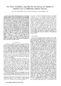
Fig. 1. Parameter sweep of the profit ratio: The blue line shows the lower bound to the energy and makespan Pareto front. The shaded region shows the power constraint with Pmax = 55 kW. The height of the green bars indicates profit for the corresponding schedule which increases as the profit ratio increases. The number beside the squares is the profit ratio γ. The profit upper bound (square) and lower bound (diamond) nearly overlap indicating that there is negligible loss in energy or makespan (and thus profit) from the recovery algorithm and shows that the maximum profit is tightly bounded.

Figure 2 shows the relative decrease in profit between the upper bound and the lower bound. Each experiment uses 100 random bag-of-tasks where the task type for each task is sampled from the original task type distribution. The probability distribution for the relative decrease in profit per unit time is shown for each experiment. The width of the glyphs represent the normalized probability density of the relative profit decrease. The figure repeats this experiment for three different bag sizes represented as the average number of tasks per machine and profit ratios. The values of γ were chosen based on Fig. 1. The maximum profit solution for γ = 1.01 minimizes energy alone while γ = 1.5 forces makespan to be minimized. The point where γ = 1.2 is roughly in the knee of the curve where neither minimizing only makespan or energy will find the maximum profit schedule. The average number of tasks per machine is shown on the x-axis. The y-axis shows the relative decrease in profit per unit time from the LP-based upper bound and the full allocation based lower bound. The lower the relative profit decrease, the better the approximation, and likewise, the tighter the optimal solution is bounded. As the number of tasks per machine increases, the quality of the solution improves. For γ = 1.5, minimizing makespan is the primary focus, which is more difficult than minimizing the energy. The bounds are tighter for lower profit ratios because energy is easier to minimize. Not only does the maximum profit algorithm produce high quality solutions but it does so extremely quickly. To find the maximum profit schedule for 10,000 tasks it takes 3.6 ms, 100,000 tasks it takes 8.9 ms, and 1,000,000 tasks it takes 74 ms. The run times are roughly linear in the number of tasks and extremely fast in all cases consider here.

B. No Idle Power For the results in this subsection, machines are modeled with no idle power consumption meaning they are turned off when not in use. In Section V-C the affect of non-zero idle power is considered. Figure 1 shows different maximum profit solutions by sweeping the profit ratio. The profit ratio is proportional to the price per bag. The profit ratio is given by the number at the bottom left of each solution. The figure shows the energy and makespan of the maximum profit solution for a given profit ratio for the full allocation and for the upper bound solution from the LP problem. Notice that the upper bound and the corresponding full allocation are very close to each other. This means that the profit per unit time is very well bounded. The overall vertical length of the green bar above each solution is proportional to the profit per unit time corresponding to that schedule. The profit increases as the profit ratio increases. The knee of this curve is interesting because neither optimizing for energy or makespan alone will produce optimal profits. Also shown in Fig. 1 is a power constraint given by the dashed line and the shaded region. When Pmax is set to 55 kW the solutions within the shaded region satisfy the power constraint.

C. Idle Power and Negative Profit To understand the effect of the idle power consumption on the algorithms, experiments were performed with the idle power set to 5% of each machine’s average power con APC sumption. Specifically, this means APC ∅j = 0.05 ij . i T This is appropriate, for example, when modeling very-low

600

1000

max profit algorithm max profit from Pareto front

0 10

profits

relative profit decrease 

15

Γ1.01 5

Γ1.2 Γ1.5

1000 2000 3000

0

0.90

13.9

138.9

1388.9

0.92

0.94

0.96

0.98

1.00

1.02

Γ

avg. tasksmachine

Fig. 4. Profit from the maximum profit algorithm and the maximum profit from the Pareto optimal solutions: The max profit algorithm finds a higher profit solution than the maximum profit solution from the Pareto front for γ < 1.

Fig. 2. Probability distributions of the relative decrease in profit per unit time from the upper bound to the lower bound for various number of tasks and profit ratios: As the bag size increases the accuracy of the maximum profit solution improves. The quality of the solution is highest when the profit ratio is small.

Figure 4 shows the profit per unit time computed from the algorithm in Section IV and the Pareto-based approach. The maximum profit solution from the Pareto front is lower than the solutions generated by the maximum profit algorithm when γ < 1. The profit is also negative for γ < 1. For γ ≥ 1 the max profit solution from Section IV is equal to the max profit solution along the Pareto front. Figures 5(a) to 5(c) show the profit and the feasible solution space for profit ratios of 0.9, 1.2, and 1.5 respectively. The contours show equi-profit lines. The black line shows the boundary of the convex feasible region. Specifically, this region is the convex set defined by the constraints of (7). This convex set is in the space of x and is projected onto the energy and makespan subspace. This projection was computed with the convex hull method described in [20]. When there is no idle power it is feasible to increase the makespan indefinitely when a minimum energy solution is sought. For this reason, without idle power the boundary of the feasible region and Pareto front have an asymptote that has infinite makespan at the minimum energy. The same affect causes the boundary of the feasible region to have an asymptote that has infinite energy at the minimum makespan solution. However, this is not the case when idle energy is used. As the makespan increases so does the energy, thus the feasible region shown in Figs. 5(a) to 5(c) is more restrictive than with no idle energy. Figure 5(c) has a high price per bag so the maximum profit solution would minimize makespan. Positive profits are not achievable in Fig. 5(a) because the profit ratio is less than unity. The non-linearity in the objective function can be seen by the lack of parallel profit contours. The minimal loss solution in this case actually tries to increase both makespan and energy. The optimal schedule slows down the processing of tasks to utilize only the most efficient machines while simultaneously decreasing the power consumption (operating expenses). This explains why a maximum profit solution is not necessarily Pareto efficient in energy and makespan.

140 makespan min

0.9

120

0.95

100

Pareto front lower bound

80

max profit upper bound

1.

60

1.05

max profit full allocation 1.1

1.2

40 174

176

178

1.35

180

182

1.5

184

186

energy MJ

Fig. 3. Parameter sweep of the profit ratio with 5% idle power: The red bars indicate a negative profit (i.e. loss) that are not along the energy and makespan Pareto front.

power sleep states. The methodology used here extends to any amount of idle power from very-low power sleep states to the significantly higher power used by low frequency P-states [19]. For very high idle power consumption, the optimal schedule will always minimize makespan because in doing so energy will also be minimized, thus maximizing profit. Similar to Fig. 1, Fig. 3 shows the energy, makespan, and profit for various profit ratios. The red bars indicate a negative profit or loss. The size of the downward bar indicates the magnitude of the loss. Schedules with negative profit might need to be realized in situations where a service level agreement (SLA) is in place requiring the users’ workload to be processed in spite of the loss. The loss might be caused by momentary increases in energy prices or maintenance that takes some machines offline. In any case, the schedule that minimizes the loss to the organization is highly desirable. When an SLA is not in place, the organization should choose to not process any tasks until a positive profit is once again achievable (γ > 1). Solutions that have a loss in profit depart from the energy and makespan Pareto front as shown in Fig. 3. This is somewhat counter-intuitive so further explanation is necessary. The key to understanding this behavior lies in the fact that (10) is not optimizing profit but rather profit per unit time. This distinction is what makes the objective function more realistic but also non-linear.

VI. M ODEL E XTENSIONS As mentioned in Section II there are other costs associated with operating an HPC system besides the cost of electricity. If conditioned power (uninterruptible power supply often with a

601

solutions are along the energy and makespan Pareto front when there is positive profit. The profit can be negative when there is idle power consumption and the price per bag is sufficiently low. In this negative profit case, the proposed algorithm still finds the maximum profit solution which is not on the energy and makespan Pareto front. As mentioned earlier, the price per bag in practice fluctuates based on the market. This research can be extended to model a dynamic price per bag by taking into account backlog and dynamic energy costs. This algorithm is fast enough that it can also be used for online batch scheduling where the tasks arrive randomly and the algorithm must determine on the fly how to assign tasks to machines.

profits 10 000

0

10 000

20 000

140

140

140

120

120

120

100

100

100

80

80

80

60

60

60

40

40

175

180

185

(a) γ = 0.9

190

175

180

185

(b) γ = 1.2

190

40

30 000

175

180

185

190

(c) γ = 1.5

Fig. 5. Profit per unit time for three different profit ratios: The x-axes is energy in mega joules and y-axes is makespan in minutes. The region within the curved line is the feasible region. When the price is low the optimal solution is along the top part of the feasible region which is not on the energy and makespan Pareto front.

ACKNOWLEDGMENTS This work was supported by the Sjostrom Family Scholarship, Numerica Corporation, and the National Science Foundation (NSF) under grant CCF-1302693. Special thanks to Ryan Friese and Bhavesh Khemka for their valuable comments.

backup generator) is used then the effective cost for electricity should be increased accordingly. Cooling of HPC systems can consume as much energy as the machines themselves depending on their geographic location and environment. Power usage efficiency (PUE) is a common metric used to represent the efficiency of the infrastructure within a data center. PUE is equal to the ratio of raw power to the power incident on the servers. PUE must be above one and typically is below two. To account for these inefficiencies, AP C can be scaled by PUE. There may be an overhead cost, oh, associated with each bag-of-tasks to cover billing activities or book-keeping. These overhead costs can be modeled by subtracting oh/MS (x) from the profit per unit time. The wear and tear on the servers can also be modeled. Let wear j be the maintenance cost per unit time of operating a machine of type j, then the effect of this cost can be modeled by subtracting  j Fj Mj wear j (11) MS (x)

R EFERENCES [1] T. D. Braun, H. J. Siegel, N. Beck, L. L. B¨ol¨oni, M. Maheswaran, A. I. Reuther, J. P. Robertson, M. D. Theys, B. Yao, D. Hensgen, and R. F. Freund, “A comparison of eleven static heuristics for mapping a class of independent tasks onto heterogeneous distributed computing systems,” Journal of Parallel and Distributed Computing, vol. 61, no. 6, pp. 810 – 837, 2001. [2] J. Koomey, “Growth in data center electricity use 2005 to 2010,” Analytics Press., vol. 1, 2011. [3] K. M. Tarplee, R. Friese, A. A. Maciejewski, and H. J. Siegel, “Efficient and scalable computation of the energy and makespan pareto front for heterogeneous computing systems,” in Federated Conference on Computer Science and Information Systems, Workshop on Computational Optimization, 2013, pp. 401–408. [4] R. Friese, T. Brinks, C. Oliver, H. J. Siegel, and A. A. Maciejewski, “Analyzing the trade-offs between minimizing makespan and minimizing energy consumption in a heterogeneous resource allocation problem,” in INFOCOMP, The Second International Conference on Advanced Communications and Computation, 2012, pp. 81–89. [5] R. Friese, B. Khemka, A. A. Maciejewski, H. J. Siegel, G. A. Koenig, S. Powers, M. Hilton, J. Rambharos, G. Okonski, and S. W. Poole, “An analysis framework for investigating the trade-offs between system performance and energy consumption in a heterogeneous computing environment,” in IEEE 27th International Parallel and Distributed Processing Symposium Workshops (IPDPSW), Heterogeneity in Computing Workshop. IEEE, 2013, pp. 19–30. [6] R. Friese, T. Brinks, C. Oliver, H. J. Siegel, A. A. Maciejewski, and S. Pasricha, “A machine-by-machine analysis of a bi-objective resource allocation problem,” in International Conference on Parallel and Distributed Processing Technologies and Applications (PDPTA), 2013. [7] L. Rao, X. Liu, L. Xie, and W. Liu, “Minimizing electricity cost: Optimization of distributed internet data centers in a multi-electricitymarket environment,” in IEEE INFOCOM, 2010. [8] D. Le, J. Chang, X. Gou, A. Zhang, and C. Lu, “Parallel AES algorithm for fast data encryption on GPU,” in Computer Engineering and Technology (ICCET), 2010 2nd International Conference on, vol. 6, April 2010. [9] A. Iosup and D. Epema, “Grid computing workloads,” Internet Computing, IEEE, vol. 15, no. 2, pp. 19–26, March 2011. [10] V. Bharadwaj, T. G. Robertazzi, and D. Ghose, Scheduling Divisible Loads in Parallel and Distributed Systems. Los Alamitos, CA, USA: IEEE Computer Society Press, 1996. [11] K. Jansen and L. Porkolab, “Improved approximation schemes for scheduling unrelated parallel machines,” Mathematics of Operations Research, vol. 26, no. 2, pp. 324–338, 2001.

from the profit per unit time. Purchasing of hardware can be modeled as a depreciation. Let cost j and λj be the purchase price and mean time to failure of machine type j respectively. To model this one can subtract  Mj cost j (12) λj j from the profit per unit time. All of these operating expenses simply modify the objective function of (7) and can be converted to a linear optimization problem similar to (10). VII. C ONCLUSIONS AND F UTURE W ORK As the operating costs of HPC systems grow, new scheduling algorithms are necessary to incorporate these costs into the task scheduling process. This work incorporates the concept of profit into HPC scheduling. A novel algorithm was presented that efficiently computes a near-optimal profit schedule. This algorithm computationally scales very well as the number of tasks grows. In addition, the quality of the solution actually improves as the problem size increases. The maximum profit

602

[12] A. M. Al-Qawasmeh, A. A. Maciejewski, H. Wang, J. Smith, H. J. Siegel, and J. Potter, “Statistical measures for quantifying task and machine heterogeneities,” The Journal of Supercomputing, vol. 57, no. 1, pp. 34–50, 2011. [13] G. Eichfelder, Adaptive Scalarization Methods in Multiobjective Optimization. Springer, 2008. [14] D. Bertsimas and J. N. Tsitsiklis, Introduction to Linear Optimization, ser. Optimization and Neural Computation. Athena Scientific, 1997. [15] R. Graham, “Bounds on multiprocessing timing anomalies,” SIAM Journal on Applied Mathematics, vol. 17, no. 2, pp. 416–429, 1969. [16] (2013, May) Intel core i7 3770k power consumption, thermal. [Online]. Available: http://openbenchmarking.org/result/1204229-SU-

CPUMONITO81 [17] K. M. Tarplee. (2013, November) Maximum profit optimization data. [Online]. Available: http://goo.gl/v05Tyo [18] (2013, March) Coin-or clp. [Online]. Available: https://projects.coinor.org/Clp [19] D. Li and J. Wu, “Energy-aware scheduling for frame-based tasks on heterogeneous multiprocessor platforms,” in 41st International Conference on Parallel Processing (ICPP), 2012, pp. 430–439. [20] T. Huynh, C. Lassez, and J.-L. Lassez, “Practical issues on the projection of polyhedral sets,” Annals of Mathematics and Artificial Intelligence, vol. 6, no. 4, pp. 295–315, 1992.

603