Energy-based Routing and Cruising Range Estimation for Electric Bicycles Simon Tobias Haumann University of Vienna Working Group Cartography and Geoinformation Sciences Universitätsstraße 7 Vienna, Austria
[email protected]
Dominik Bucher ETH Zürich Institute of Cartography and Geoinformation Stefano-Franscini-Platz 5 Zurich, Switzerland
[email protected]
David Jonietz ETH Zürich Institute of Cartography and Geoinformation Stefano-Franscini-Platz 5 Zurich, Switzerland
[email protected]
Abstract Electric bicycles offer a convenient transport alternative for short to medium distance travels. Due to their small size, low cost, and environment-friendly nature, the number of sold bikes is increasing steadily, not only for private use, but also for company fleets, free-floating mobility systems, and bike-sharing providers. This increment leads to an increased need for planning systems. On the one hand, people are interested in knowing which routes to take in order to maximize the distance they can drive with a certain battery charge. On the other hand, it is becoming increasingly important to predict the cruising range in a situational context, including road network properties, personal preferences and restrictions, or weather conditions. This information is not only valuable for individual users, but also for fleet managers, who need to recharge, move and replace bicycles. We propose a novel static energy model for electric bicycles, which allows us to compute energy requirements for arbitrary street segments, given contextual information such as the road network, a digital elevation model (DEM), and parameters like weight, desired speed, or the presence of a recuperation mechanism. This model is embedded within a routing application, which can be used to compute the route with the lowest energy demand or farthest cruising range estimations. We used this application together with data collected from several test rides to estimate and validate the model parameters. Keywords: routing, e-mobility, consumption model, electric bicycle, reachability.
1
Introduction
As cities become more densely populated due to a rising urbanization, and societies try to decrease the dependency on fossil energy sources, it is increasingly important to substitute many of the trips previously covered by car with smaller and more energy-efficient modes of transport. Electric bicycles fit nicely into this gap, as they take little space on the roads, may be fueled by renewable energy, and decrease physical strain as compared to a regular bicycle (thus increasing the personally reachable range). Those advantages manifest themselves in growing sales numbers, electric bike fleets in companies and emerging station-based and free-floating e-bike systems within cities (Paul & Bogenberger 2014). This increment also makes it increasingly important to be able to effectively assess driving ranges of bicycles taking into account not only parameters of the bike itself, but also of the person using it, the roads available for travel, and any other contextual data that may influence the journey. Based on a variety of other electrical and physical consumption models (cf. Hoch 2015; Abagnale et al. 2015), we built a model of an electrical bicycle, which is embedded in a framework for route computations on static models. This framework features a processing pipeline tailored to fast querying for electrical bicycle routes. Prominent steps in the
pipeline are the evaluation of multiple parameters in parallel, and building up static cost graphs based on a road network and a digital elevation model (DEM). Those calculations are followed by query preparation and storage in a database, which is then used within a fast routing system, able to query graphs with negative edge weights. Finally, a prototypical application is built with the aim of route planning and cruising range estimation. Many of the model parameters presented in this study were measured or taken from literature and the bicycles’ specifications, such as the wheel radius, or the battery capacity. In order to determine others, we conducted preliminary field tests with electric bicycles, which allowed us to tune the remaining parameters, such as the motor efficiency, and provide a first step towards validating the model.
2
Related Work
The profound potential for energy-based routing has previously been stated by Ericsson et al. (2006), initially in reference to fossil fuel use and later with specific regard to electric vehicles (EV) (Sachenbacher et al. 2011). For EVs in particular, this routing approach will gain even more importance in the future, with range anxiety and long recharge
AGILE 2017 – Wageningen, May 9-12, 2017
times still representing major user concerns (cf. Neaimeh et al. 2013; Artmeier & Haselmayr 2010). A large body of work covers similar energy models for electric cars (Hoch 2015; Oliva et al. 2013), both from an engineering point of view (e.g., to assess the influence of different parts on the overall energy consumption), as well as for routing and cruising range estimation (Neaimeh et al. 2012; Neaimeh et al. 2013). While these models are to a large degree applicable to the topic of electric bicycles as well, there are several differences: the smaller complexity of the drivetrain (e.g., less auxiliary components), the additional power supplied by the rider, or the lack of battery temperature management (cf. Yuksel & Michalek 2015; Li et al. 2016). For example, the recent research on electric bicycle energy models by Abagnale et al. (2015) only consists of a motor and gearbox in sequence. The recuperation mechanism prevents the use of a routing algorithm such as the Dijkstra algorithm (Dijkstra 1959) or the A* algorithm (Hart et al. 1968), as the battery may be charged during a downhill segment, thus representing negative edge weights. While Dijkstra (and its variations) assume that all edge weights are non-negative, the Bellman-Ford algorithm
(Bellman 1958) offers an alternative as it is able to overcome this limitation. As models for electrical bicycles are largely dependent on personal parameters (e.g., weight, rider power supply), heavy pre-processing prevents us from updating edge weights dynamically. While recent research has shown methods for dynamic graph updates (e.g., Schultes & Sanders 2007), it usually focuses on updating only a few edges. For that reason, we opted for building a processing pipeline, which computes multiple parameterized graphs in parallel.
3
Energy Model
An electric bicycle powertrain has to supply enough energy to overcome gravitation, drag, and friction (i.e., road resistance). Steep slopes cause a large gravitational force, which can either lead to energy consumption (when going uphill), or energy production (when going downhill): (1)
𝐹𝑔 = 𝑚 ⋅ 𝑔 ⋅ sin(𝛼)
Figure 1: The beginning of the energy consumption model. It contains all model parameters followed by several data preparation stages (which include automated data retrieval, and pre-processing of the street graph).
AGILE 2017 – Wageningen, May 9-12, 2017
In this formula, m is the total mass (i.e., bicycle and rider), g is the gravitational constant, and is the slope angle. The drag or air resistance is commonly defined as: 𝐹𝑑 =
(2)
𝑃𝑎𝑚𝑏 2𝑅𝑎 𝑇𝑎𝑚𝑏
𝑐𝑤 𝐴(𝑣𝐷𝐷 − 𝑣𝑤𝑥 )2
Here, Pamb denotes the ambient air pressure, Ra the universal gas constant, Tamb the ambient temperature, cw the drag coefficient, A the reference area, vDD the driving speed in driving direction and vwx an optional wind speed. For simplicity, we assume the wind speed to always be zero in our implementation. Finally, the definition of friction is (which is proportional to the gravitational force with a friction coefficient crr): (3)
(4)
𝐹ℎ = 𝐹𝑇 ⋅ 𝛾
Accordingly, the overall wheel torque 𝑇𝑣 consists of 𝑇𝐸𝑀 + 𝑇ℎ , where 𝑇𝐸𝑀 is the motor torque. The above forces induce a certain torque on the wheels, denoted as 𝑇𝑣 = 𝐹𝑇 𝑟𝑤 , where rw is the wheel radius. Using the angular velocity of the wheel (𝑤𝑣 = 𝑣𝐷𝐷 /𝑟𝑤 ), the equation for motor power generation / consumption results in formula (5). 𝑃𝑖 denotes the energy expenditure of auxiliary components.
𝐹𝑓 = 𝑐𝑟𝑟 ⋅ 𝑚 ⋅ 𝑔 ⋅ cos(𝛼)
Power generated via the electric powertrain has to overcome all these forces (𝐹𝑇 = 𝐹𝑔 + 𝐹𝑑 + 𝐹𝑓 ), in order to propel the bicycle forward. Note that we are omitting the so-called acceleration resistance, which is used to model how a vehicle accelerates and decelerates. Instead, a measured average velocity is assumed to be the prospective target velocity. There are different systems for controlling the ratio between rider and motor power input. For example, Abagnale et al. (2015) propose the pedelec velocity control (PVEC), in which the motor provides full support up to a selectable target velocity. Since this method only works in a dynamic model, we instead model the rider power input 𝐹ℎ as a constant factor of the tractive force 𝐹𝑇 , depending on the chosen power level. Ultimately, the maximal rider power supply is also limited by a user-dependent value.
Figure 3: Exemplary part of the model. It shows the computation of drag in Python as well as the iteration different velocity levels for the entire model. (2) !pressure_hPa!*100/(2*287.058*(%temperature_celsius%+273.15)) *1.15*0.55*math.pow((%velocity_kmh%/3.6),2) #drag
Figure 2: Bellman-Ford application with a reachability request. The example shows the maximum remaining cruising range with a SOC of 20 Wh from an arbitrary location in Zurich.
AGILE 2017 – Wageningen, May 9-12, 2017
𝑇𝐸𝑀 𝑤𝑣
(5)
𝑃𝐸𝑀 = {
𝜂𝐸𝑀 (𝑇𝐸𝑀 ,𝑤𝑣 )⋅𝜂𝐺
𝑇𝐸𝑀 𝑤𝑣 ⋅ 𝜂𝐸𝑀 (𝑇𝐸𝑀 , 𝑤𝑣 ) ⋅ 𝜂𝐺 +
Where EM is the motor efficiency (depending on torque and velocity) and 𝜂𝐺 the gearbox efficiency. For torques greater than zero, the motor is in consumption mode, and for torques smaller than zero, it is in production mode. For bicycles, which lack a recuperation system, the motor simply never operates in production mode, i.e., PEM will never be negative, and the battery will never be recharged. In our model, this restraint is a parameter of the bicycle, which limits PEM accordingly. As most people charge their battery indoors, i.e., in a warmer environment, the power consumption appears to be larger due to the battery cooling down. The effect of the battery cooling down is approximated by a temperature-dependent factor , to be measured empirically: (6)
𝑃𝑀 = 𝑃𝐸𝑀 ⋅ (1 + (25 − Δ𝑇𝑎𝑚𝑏 ) ⋅ 𝛽)
The electric motor power ultimately results in the energy consumption required for each road segment of length 𝑙: (7)
4
𝐸𝐸𝑀 = 𝑃𝑀 ⋅
+ ∑𝑛𝑖=1 𝑃𝑖
𝑙 𝑣𝐷𝐷
Routing Application
To find routes with low energy consumptions, the model from Section 3 must be applied to a street network. Such a network is typically described as a graph, consisting of nodes (i.e., street intersections), which are connected by edges (i.e., streets, bike lanes, etc.). Such a model application either computes all required values dynamically during the routing process, or builds a static graph of edge costs. Our model
∑𝑛𝑖=1 𝑃𝑖
𝑇𝐸𝑀 ≥ 0 𝑇𝐸𝑀 < 0
follows the second approach, as routing on a static graph is much less computationally intensive, and thus applicable for large graphs, such as a street network. The recurrence of numerous personalized input parameters in different stages of the cost calculation process makes it almost impossible to fully process the model dynamically upon request resp. would lead to unacceptable query times.
4.1
Edge Cost Calculation
We transformed the conceptual approach for an energy model from Section 3 into a programmatic model using ArcGIS Model Builder. Zurich City was chosen as survey area, because it contains a dense road network and steep and flat regions. However, a later adaption and optimization could easily be performed by changing input parameters for any desired location. The graph building application consists of the following stages, which are built as an automated data pipeline: road network preparation, extraction of altitude values from a DEM, calculation of intermediate model values (impeding forces, wheel torque and angular velocity), and computation of electrical motor power and energy consumption. Naturally, all edge costs have to be computed both for a forward and backward traversal, for different bike parameters (i.a. recuperation mode switched on or off), and different target velocities (cf. Figure 1 and Figure 3). The data conditioning stage from Figure 1 defines a routing topology, which uses certain constraints (request predicate to include negotiable roads only, as well as the use of a configuration file optimized for bicycles), followed by altitude extraction on each node of the network. The defined goal is to fully automate the model (i.a. DEM through ArcREST). However, to ensure the best possible evaluation and model
Figure 4: Bellman-Ford application with a routing request from ETH Hönggerberg to ETH Centre. Note the difference to the modelled value in Table 2, caused by recuperation in downhill segments.
AGILE 2017 – Wageningen, May 9-12, 2017
optimization thereafter we used the swissALTI3D from swisstopo with a resolution of 2m. Each quantity is calculated according to the equations from Section 3. For example, Figure 3 shows the computation of drag in the model, as transformed from the theoretic approach from Section 3 (2). The iteration in the model allows us to calculate energy consumption at multiple velocity levels and match them with the actual average speed while moving (cf. Section 4.3).
4.2
Application
In a first step, for bikes without recuperation and thereby generating only positive edge costs, we compute routes with pgRouting (PostgreSQL) using the Dijkstra algorithm. Second, our own development of a routing application using an implementation of the Bellman-Ford algorithm (Bellman 1958) written in Rust enables us to involve negative edge costs caused by an energetic recovery system henceforth (Figure 2 and Figure 4).
4.3
Evaluation
To tune the model, we ran repetitive test drives on three routes (Figure 5). The tests were carried out with adapted input parameters, i.a. considering the specific temperature on that day and the weight of the subject. Therefore, we can distinguish between constant, model depending arguments and those of a more dynamic nature. Several parameters that we did not measure on our own were assumed as approximation values from literature (Table 1).
Table 1: The model parameters. Model Parameter Value Table 2 weight 𝑚 driver [kg] 23 e-bike [kg] Table 2 temperature 𝑇𝑎𝑚𝑏 [celsius] 9.806 standard gravity 𝑔 [m/s2] modelslope angle [degree] dependent 0.003 rolling coefficient 𝑐𝑟𝑟 ambient air pressure 𝑃𝑎𝑚𝑏 [hPa] universal gas constant 𝑅𝑎 drag coefficient 𝑐𝑤 reference area 𝐴 [m2] velocity levels 𝑣𝐷𝐷 [km/h] factor torque 𝛾
modeldependent 287.058
wheel diameter (resp. wheel radius rw) [inches] motor efficiency 𝜂𝐸𝑀
28
gearbox efficiency 𝜂𝐺
0.98
gradeability [degree] temperature-dependent factor
15 0.0047
auxiliary components 𝑃𝑖 [W]
1.08
0.55 1.15 15, 20, 25 (Table 2) 0.1
0.45
Reference producers specs Measured
Wilson (2004); adjusted empirically
Wilson (2004) Wilson (2004) model iteration empirical approximation producers specs
producers specs; adjusted empirically Abagnale et al. (2015) producers specs producer specs; empirical approximation producers specs
AGILE 2017 – Wageningen, May 9-12, 2017
Figure 5: Test Tracks. The Map shows all routes from Table 2 with the modelled energy consumption per street segment. It compares the calculated energy-based routes with the shortest routes.
Representing the majority of electric bicycles currently available, we employed a bike without recuperation mechanism for the first series of tests. For each test drive, the route and average speed were tracked and matched with modelled values afterwards. We used the highest power level to exploit full potential of the electric motor, while later integration of different assistance levels into the model remains possible. Through a retroactive approach, we ascertained energy consumption in recharge mode using an energy cost meter at the respective target location. This procedure is illustrated by plugs in Figure 5, which shows energy demand for each street segment, compared to the deviation of the shortest route additionally. Using data recorded during the test drives, we tuned i.a. motor efficiency and the rolling resistance coefficient, to increase the model fit. Out of five repetitive test drives on the three routes, the average deviation between measured and modelled values is around 7 %. Table 2 shows an example for the gathered data for one session comparing measured and modelled values.
Table 2: A Test Drive Session with adapted parameters from Table 1. Origin - Target Energy Consumption[Wh] (𝑚=100; 𝑇𝑎𝑚𝑏 =3; 𝑣𝐷𝐷 =20) Measured Modelled Bülachhof – ETH 85 86 Hönggerberg ETH Hönggerberg – ETH 48 46 Centre ETH Centre – Bülachhof 41 40
AGILE 2017 – Wageningen, May 9-12, 2017
5
Discussion and Future Work
We presented a static e-bike model, an automated processing pipeline for route graph building, and a host application, which can be used for route planning, navigation systems, reachability analyses, or urban planning, e.g., for the designation of new bicycle routes or to determine the locations of new e-bike stations in a bike sharing system. In particular, applications where fast querying on a personalized graph is necessary benefit from our approach. Furthermore, by adjusting the parameters and the overall setting, the model can be used for other EVs. Currently, we are carrying out additional test drives with different electric bicycles capable of recuperation, to determine parameters more accurately and evaluate the overall model applicability. For example, our modeling of human power input and temperature influence will need further empirical validation. Objectives for additional research are automation, optimization, and refinement of the model, such as the inclusion of traffic and street type data, parameters which determine acceleration/deceleration phases (e.g., traffic lights or pedaling frequency and strength), or a more detailed state of charge (SOC) model. Our eventual goal is to develop an application for real-time navigation systems, which is able to switch from shortest route into energy-saving mode – knowing the required energy for the remaining distance. Consequently, a previously assumed inaccessible target at a certain low SOC could still be reached.
Hart, P.E., Nilsson, N.J. & Raphael, B. (1968) A Formal Basis for the Heuristic Determination of Minimum Cost Paths. IEEE Transactions on Systems Science and Cybernetics, 4(2), pp.100–107. Hoch, N. (2015) Customer-Centric Travel Planning for Electric Vehicles. ETH Zürich. Li, W., Stanula, P., Egede, P., Kara, S. & Herrmann, C. (2016) Determining the Main Factors Influencing the Energy Consumption of Electric Vehicles in the Usage Phase. Procedia CIRP, 48, pp.352–357. Neaimeh, M., Higgins, C., Hill, G., Hübner, Y. & Blythe, P. (2012) Investigating the effects of topography and traffic conditions on the driving efficiency of Electric Vehicles to better inform smart navigation. In IET and ITS Conference on Road Transport Information and Control (RTIC 2012). Institution of Engineering and Technology, pp. 1–6. Neaimeh, M., Hill, G., Hübner, Y. & Blythe, P. (2013) Routing systems to extend the driving range of electric vehicles. Intelligent Transport Systems, IET, 7, pp.327–336. Oliva, J.A., Weihrauch, C. & Bertram, T. (2013) A ModelBased Approach for Predicting the Remaining Driving Range in Electric Vehicles. Annual Conference of the Prognostics and Health Management Society, pp.438–448.
References
Paul, F. & Bogenberger, K. (2014) Evaluation-method for a Station Based Urban-pedelec Sharing System. Transportation Research Procedia, 4, pp.482–493.
Abagnale, C., Cardone, M., Iodice, P., Strano, S., Terzo, M. & Vorraro, G. (2015) A dynamic model for the performance and environmental analysis of an innovative e-bike. Energy Procedia, 81, pp.618–627.
Sachenbacher, M., Leucker, M., Artmeier, A. & Haselmayr, J. (2011) Efficient Energy-Optimal Routing for Electric Vehicles. Proc. Twenty-Fifth AAAI Conference on Artificial Intelligence, pp.1402–1407.
Artmeier, A. & Haselmayr, J. (2010) The optimal routing problem in the context of battery-powered electric vehicles. Workshop: CROCS, pp.1–13.
Schultes, D. & Sanders, P. (2007) Dynamic highway-node routing. Experimental Algorithms, pp.66–79.
Bellman, R. (1958) On a Routing Problem. Quarterly of Applied Mathematics, 16, pp.87–90. Dijkstra, E.W. (1959) A Note on Two Probles in Connexion with Graphs. Numerische Mathematik, pp.269–271. Ericsson, E., Larsson, H. & Brundell-Freij, K. (2006) Optimizing route choice for lowest fuel consumption Potential effects of a new driver support tool. Transportation Research Part C: Emerging Technologies, 14, pp.369–383.
Wilson, D.G. (2004) Bicycling Science, Massachusetts Institute of Technology.
Cambridge:
Yuksel, T. & Michalek, J.J. (2015) Effects of regional temperature on electric vehicle efficiency, range, and emissions in the united states. Environmental Science and Technology, 49, pp.3974–3980.