Energy-Constrained Performance Optimizations For Real-Time ...

Energy-Constrained Performance Optimizations For Real-Time Operating Systems Tarek A. AlEnawy and Hakan Aydin Computer Science Department George Mason University Fairfax, VA 22030

{thassan1,aydin}@cs.gmu.edu However, an almost invariable assumption of this line of research is that the “hard” performance constraint for the operating system is still to meet all the task deadlines, and that minimizing the energy consumption subject to hard real-time constraints is a highly desirable, yet “secondary”, performance objective. In this paper, we look at the problem from the other perspective: we consider systems with “hard” energy constraints. That is, we assume that we are given a limited/scarce energy budget (Ebudget) and a targeted system run time (mission time) during which the system must remain functional. Such a situation can arise when the computing device depends on the battery power supply during the operation, example scenarios include embedded control applications as well as military, space, and disaster recovery missions where a predictable realtime system behavior is necessary but battery re-charging during the mission is not possible (or feasible) at all. In fact, this is exactly one of the main arguments of [9], where the authors focus on the case of Mars Rover system to argue about the need to promote the ‘hard’ energy constraint to a first-class design consideration. Having the knowledge of the workload and the energy limitations, the operating system is often the entity that is in best position to plan for delivering maximum performance within the available energy budget. Clearly, the operating system can still make use of well-known power-aware realtime scheduling techniques (such as DVS or predictive shutdown) and compute the minimum energy (Ebound) required to meet all the deadlines during the mission time. However, in scarce-energy settings where Ebudget < Ebound , we have a serious problem: some deadlines will inevitably have to be missed. As we show in section 3 through a simple example, without any provisions, the system may run out of energy in the middle of the operation with no control whatsoever on the specific deadlines missed. In contrast, in our approach the operating system selectively labels task instances as ‘skipped’ or ‘selected’, prior to task execution, in order to stay within the energy budget while maximizing the performance. At run-time, only the task instances (jobs) that have been previously selected by the operating system are dispatched.

ABSTRACT In energy-constrained settings, most real-time operating systems take the approach of minimizing the energy consumption while meeting all the task deadlines. However, it is possible that the available energy budget is not sufficient to meet all deadlines and some deadlines will inevitably have to be missed. In this paper, we present a framework through which the operating system can select jobs for execution in order to achieve two alternative performance objectives: 1) maximizing the number of deadlines met , and 2) maximizing the total reward (utility) of jobs that meet their deadlines during the operation. We present an optimal algorithm that achieves the first objective. We prove that achieving the latter objective is NP-Hard and propose some fast heuristics for this problem. We evaluate the performance of the heuristics through simulation studies.

Keywords Real-time scheduling, real-time operating systems, energy management, power-aware scheduling, power-aware systems.

1. INTRODUCTION With the proliferation of wireless, portable and embedded devices, power-aware systems have moved to the forefront of Computer and Electrical Engineering research in recent years. A prominent energy management technique for real-time/embedded systems is based on Dynamic Voltage Scaling (DVS). With DVS, it is possible to obtain significant savings in CPU energy consumption by simultaneously reducing the supply voltage and the clock frequency (CPU speed) at the expense of increased latency. Thus, in recent years, the real-time DVS (RT-DVS) research has been dominated by numerous papers that address the problem of meeting task deadlines while minimizing the CPU energy consumption under various task/system models and off-line/on-line scheduling techniques [1,2,3,6,9,10,11,12,14,15,16].

4.1

defined as Ci /Pi. We denote the jth instance of task Ti by Tij , which is also referred to as the job Tij . The hyperperiod P of the task set is defined as the least-common multiple of all task periods. All the tasks are assumed to be independent and simultaneously ready at time t=0. Our framework assumes preemptive scheduling. Finally, we assume that the preemption overhead is negligibly small and, if needed, it can be incorporated into Ci .

In this research effort, we propose three performance metrics to determine the task instances (jobs) to be executed during the system operation, namely: • maximize the number of met deadlines, • maximize the number of met deadlines while providing a minimum performance guarantee for each task, and • maximize the reward (utility) of the system by giving preference to more important/critical tasks. Each of the metrics above may be more appropriate for different systems and “mission” objectives. We underline that our framework is applicable to systems with or without DVS capability. In systems where the CPU does not have the DVS capability, our framework provides a way to maximize the system performance in terms of timing constraints and criticality, while staying within the energy budget. On the other hand, DVS capability by itself does not guarantee that all the timing constraints will be met while staying within a given fixed energy budget. As an example, consider a task set with total utilization 0.9. A well-known result from RT-DVS theory states that the minimum CPU speed that minimizes the CPU energy consumption and still meets all the deadlines is equal to 90% of maximum CPU speed [2] when the scheduling policy is Earliest-Deadline-First (EDF). Now suppose that this system has to remain functional for one hour, requiring K units of energy with speed 0.9. If it is not possible to recharge the battery during the operation and if the battery in use can deliver at most K/2 energy units, then clearly the operating system has to adopt additional energy saving strategies (besides using DVS) to yield the best performance possible in these circumstances. We note that a recent study [13] has also addressed some aspects of real-time scheduling issues with a fixed energy budget. However, the model in that paper is based on tasks having identical periods, as opposed to our more common and general case of possibly different periods. In addition, we also explore the more common performance metric of minimizing the number of missed deadlines in addition to maximizing the system reward. The rest of this paper is organized as follows. In section 2 we present the system model and our assumptions. In section 3 we define the problem formally and explain our performance metrics for energyconstrained settings. Section 4 discusses the proposed solutions. In section 5, we present our simulation results. In section 6 we conclude the paper.

2.2 Power and energy consumption model Throughout the paper we distinguish between two operational modes: normal (execution) mode and lowpower (stand-by) mode. We say that the system is in normal (execution) mode when the system is executing a job. Otherwise, the system switches to low-power (standby) mode when the CPU is idle. The power consumptions of the normal mode and low-power modes are assumed to be ge and glow watts (joules per second), respectively1. In an interval [t1,t2], the total energy consumption of the CPU is the sum of the execution mode energy Ee and the lowpower mode energy Elow: (1) E (t1 , t 2 ) = Ee + Elow = g et e + g lowt low where te is the total time during which the system runs in the execution mode and tlow is the total time during which the system runs in the low-power mode in the specified interval. In our settings, the system has a limited CPU energy budget Ebudget, and moreover, it has to remain operational in the interval [0,X]; that is, the total CPU energy consumption should not exceed a pre-determined threshold Ebudget for X time units. X is also called the mission time throughout the paper. In other words, the system is subject to a hard energy constraint, which is a measure of available energy resources. The minimum energy amount necessary to complete all the task instances in a timely manner (i.e. before their deadlines) is denoted by Ebound. Throughout the paper we will assume that the task set is schedulable, that is all deadlines would be met according to a policy of designer’s choice (e.g. EDF or RMS), if the available energy were greater than or equal to Ebound (i.e., if Ebudget ≥ Ebound). We are making this assumption because our goal is not to study real-time schedulability problem in the absence of any energy constraints, an intensively studied problem [8]. Instead, our focus will be on the systems with hard energy constraints where the available energy is not sufficient to execute all the workload; that is, we consider systems where Ebudget < Ebound .

2. SYSTEM MODEL 2.1 Task model We consider a set of n periodic tasks T={T1, T2,…, Tn } that are to be scheduled on a single-processor system. Each task Ti is characterized by its worst-case execution time Ci, relative deadline Di, and period Pi which is assumed to be equal to Di . The utilization Ui of task Ti is

1

4.2

The energy overhead due to switching between the two modes can be incorporated into glow, if necessary. Similarly, the time overhead due to switching can be incorporated into Ci.

the total utilization does not exceed 1.00 [7], if we do not take into account the hard energy constraint. Figure 1 shows the schedule produced by EDF (solid arrows denote the deadlines met, whereas the dashed arrows indicate the missed deadlines). Observe that since the hard energy constraint is not taken into account, the system runs out of energy at t=1425, just before T32 completes. Due to inefficient energy management the system energy budget is exhausted just before 60% of the mission time X has elapsed, about 23% of Ebudget is wasted by executing T32 which never completes, and only 15 deadlines (about 56 % of the total) are met. Figure 2 shows an “improved” schedule (for the same problem) that intelligently uses the available energy to yield better performance. In this case, the system remains operational throughout the entire mission time and we are able to meet 21 deadlines (about 78% of the total, with 40% improvement compared to the naive schedule of Figure 1) without exceeding Ebudget. Note also that all the jobs completed in the naive schedule are still completed in the improved schedule. As this example illustrates, if the energy budget of the system cannot sustain the operation during the entire mission, then the aim must be to provide maximum predictability/utility for applications imposing timing constraints. We consider two cases of maximizing system performance in energy-constrained settings as follows.

Applicability to systems with multiple speed levels: In DVS-enabled systems with multiple frequency and power levels, it is realistic to set ge to the power consumption level of the lowest CPU speed that would be able to meet all the deadlines with the given scheduling policy. Ebound would be then equal to the energy consumption corresponding to this speed/power level during the entire mission, and our objective is again to provide a task selection framework for systems with scarce energy budget (where Ebudget < Ebound ).

3. MAXIMIZING SYSTEM REWARD IN ENERGY-CONSTRAINED SETTINGS As explained in Introduction, for some applications it may be vital that the system remain functional and does not run out of energy during the mission time interval [0,X]. Moreover, if the available energy is scarce, blindly trying to execute all the jobs may result in a rather poor performance when we consider timing constraints, as the following example illustrates.

T1

3.1 Maximizing the number of deadlines met during mission time

T2 Energy exhausted!

One natural performance objective might be to maximize the total number of deadlines met, within the limited energy budget, while sustaining the system operation during [0,X]. This is particularly suitable for applications where occasional deadline misses may be acceptable, such as real-time communications, tracking and multimedia [6,8]. We denote this objective by O1. We examine two variations of this objective. • No minimum task–level requirements:

T3 800

1600

2400

Figure 1: Naïve schedule generated by EDF

T1

In the absence of any additional constraints, we can simply try to maximize the total number of deadlines met across all tasks during mission time [0,X].

T2 Mission completed

• Minimum task deadline meet ratio:

T3 800

1600

2400

The operating system may attempt to ensure that a minimum percentage of each task’s deadlines are met during mission time [0,X], thus providing a minimum performance guarantee for each task. This can be done by requiring that each task Ti meets its minimum deadline meet ratio Mi such that ni / Ni ≥ Mi, where ni is the number of instances of task Ti that completed before their deadlines during [0,X] and Ni =  X / Pi  is the number of all the instances of the same task whose deadlines lie within the same interval. Note that the aim is still maximizing the

Figure 2: Improved schedule Example 1 Consider a task set that consists of three tasks T1 , T2 , and T3 with the following parameters: U1 = U2 = 0.25, P1= P2 = 200, C1 = C2 = 50; U3 = 0.5, P3 = 800, C3 = 400. Let Ebudget = 1425, X = 2400, ge = 1, glow = 0.025. Based on these parameters Ebound can be computed as 2400. The task set is schedulable using Earliest-Deadline-First (EDF) since 4.3

number of deadlines met; only we are adding the minimum performance constraints. In fact, the “improved” schedule of Figure 2 maximized the total number of deadlines met for the task set discussed in Example 1, subject to the constraint Mi = 30% for each task.

= 0 indicates that the job is skipped and Sij = 1 indicates that it is selected for execution. At run-time, only jobs whose labels are set to “selected” are dispatched. Let Π′ = { Tij  Sij = 1 } denote the set of selected instances. Thus the problem becomes, choose Π′ ⊆ Π to achieve the performance objective (O1 or O2) while making sure that the energy budget is not exceeded. Note that the energy consumed by the selected task instances plus the energy consumed in the stand-by mode should not exceed Ebudget . That is:

3.2 Maximizing the total reward (utility) of the system Objective O1 given in section 3.1 does not distinguish between the importance of different tasks. However, some tasks may be deemed more important than others in the presence of limited energy budget. For example, realtime communication tasks may be more important than display update tasks. To this aim, we can associate a weight (reward) wi with each task Ti. If an instance Tij is completed before its deadline, then the total system reward is increased by wi units (Note that all the jobs of Ti have the same reward). Otherwise, if an instance is skipped altogether or misses its deadline then the total reward remains the same. Thus, we have the objective O2: selectively execute jobs so as to maximize the total system reward. The two variations discussed in O1, either guaranteeing a minimum deadline meet ratio for each task or the absence thereof, can still be applied to this case. Also observe that, Objective O1 is a special case of Objective O2 where all the tasks have the same weight wi = w.

 

Tij ∈Π '

(2)



Or equivalently, (3)

g low X + ( g e − g low ) ∑ Ci ≤ Ebudget Tij ∈Π '

Note that the quantity (ge - glow)Ci is the excess energy consumed by each instance of task Ti in normal mode beyond the idle energy. Once selected, the set Π′ can be scheduled by the algorithm α and the feasibility of selected instances is guaranteed since the superset Π is assumed to be initially schedulable under Algorithm α when the energy budget is not taken into account. Task Parameters

Mission Time (X)

Optimization Module (OM)

3.3 Our approach

Determine_job_ pool

In energy-constrained settings where Ebudget < Ebound , the task instances to be executed must be carefully selected in order to make best use of available energy. Clearly, objectives O1 and O2 will provide the guidelines depending on the performance metric under consideration. To achieve this aim, the operating system can undertake a job selection phase in which each task instance (job) is labeled as skipped or selected. Clearly the operating system must consider the parameters of the task set, as well as available energy and operation duration information when making decisions in light of the performance metric of choice. Our solutions are general in the sense that they work with any scheduling policy α (e.g. RMS or EDF), providing maximum flexibility for the operating system2. Let Π be the set of all task instances (jobs) that must complete by (i.e. with deadlines on or before) the mission time X. We associate with each job Tij a label Sij where Sij 2



∑ g eCi +  X − ∑ Ci  glow ≤ Ebudget

Tij ∈Π '

{Ni}

Select_number_of_ instances_to_execute

Performance Objective (O)

Energy Budget

{ni}

Determine_job_ level_labels

{Sij}

Additional Labeling Criterion (D)

Figure 3. The generic job selection framework for energy-constrained real-time operating systems The generic job selection framework that we propose for energy-constrained real-time operating systems consists of three main modules (Figure 3): • Determine_job_pool(T, X, {Ni}): For each task Ti , calculates the total number of instances Ni whose deadlines are smaller than or equal to X. Note that Ni is simply equal to  X / Pi  , since this quantity gives the number of jobs belonging to Ti that must complete by X. • Select_number_of_instances_to_execute(T, O, X, {Ni}, {ni}, Ebudget): Uses an auxiliary optimization module OM, which can be an optimal algorithm or a heuristic, to decide on the number of instances ni to be executed for each task Ti

Recall that we assume the feasibility of the schedule is guaranteed if all the jobs run in normal-mode and scheduled by Algorithm α when there are no constraints on energy budget.

4.4

during [0,X] to achieve the specific objective O under consideration, without exceeding the energy budget. This is the only module that needs to be modified if the performance objective changes. • Determine_job_labels({ni}, D, {Sij}): Given the number of instances ni to be executed for each task Ti , determine specific instances to be actually scheduled using an additional labeling criterion D. In other words, determine the label Sij (skipped or executed) for each job. These labels will be used in conjunction with the original scheduling algorithm α at run-time, to maximize the system performance while staying within the system energy budget. The module Select_number_of_instances_to_execute is highly dependent on the specific performance metric (objective) under consideration; we will give the specific pseudo-code for this module corresponding to different metrics when discussing the solutions for optimization problems.

4. SOLUTIONS TO ENERGY CONSTRAINED PERFORMANCE OPTIMIZATION PROBLEMS In this section we discuss the solutions to maximize the performance objectives stated earlier, O1 and O2.

4.1 Objective O1: maximizing the number of deadlines met during the mission time To maximize O1 while staying within Ebudget , then the problem can be solved efficiently. Consider the policy that first orders tasks according to execution time per instance Ci and then chooses for execution the instances of tasks with smallest execution times until Ebudget is exhausted. We refer to this policy as Favor Shortest Job (FSJ)3. Optimization Module for FSJ Input: T, E_budget, X, ge, glow Output: {ni} 1. Order tasks according to their execution time (T1 represents the task with the smallest execution time); 2. In_progress = true; 3. Available = E_budget – X.glow; 4. i = 1; 5. while (In_progress==true) and (i ≤ n) 6. begin 7. z = (ge - glow). Ci; 8. if z ≤ Available then 9. begin 10. Ni =  X / Pi ; 11. ni = min{ Ni ,  Available / z  }; 12. Available = Available - ni.z; 13. end 14. else In_progress = false; 15. i = i + 1; 16. end Figure 5. Pseudo-code for FSJ optimization module

Figure 4. ‘Balanced’ distribution of skipped instances Note that determining the number of instances to be executed during the mission time, namely ni, for each task is only a part of the problem. We need to determine which specific instances will be labeled as selected or skipped. As an example, suppose that a given task Ti has 200 instances during the mission, but only 150 have been selected for execution. Which 150 will be selected? The first 150, the last 150, or any 150? The labeling criterion D essentially provides the algorithm to be used for making this decision. In the simplest case, one can adopt trivial techniques such as selecting the first ni instances. However, many applications including multimedia and real-time communication tasks, would still deliver a performance of acceptable quality if the deadline misses are relatively few and distantly spaced [5,6]. Thus, in the above example, one can select three task instances out of each four consecutive instances for execution to obtain a ‘balanced’ distribution of 50 skipped instances during mission time. Part of this schedule is shown in Figure 4 (solid arrows and dashed arrows denote the met and missed deadlines, respectively). We note that the approach of meeting mi deadlines of each ki consecutive instances was previously adopted in overloaded (but not energy-constrained) real-time scheduling approaches [5,6]. We believe that this is a noteworthy parallelism between overloaded and energyconstrained systems.

Consider the select_number_of_instances_to_execute module which uses the optimization module FSJ_OP corresponding to FSJ (Figure 5). FSJ_OP starts off by setting aside enough energy to sustain the system in lowpower mode in [0,X]. All the instances of a given task Ti have the same execution time Ci , thus we can start with the task T1 having the smallest execution time C1 . Then, 3

Note that this scheme is different from the well-known scheduling algorithm Shortest Job First (SJF), because FSJ selects task instances for execution in off-line fashion, and then these instances are scheduled using the algorithm α chosen by the operating system.

4.5

FSJ_OP determines the maximum number of instances n1 of task T1 that can be executed within the current budget Ebudget . It then updates Ebudget by deducting the excess energy consumed by the newly selected jobs. This process is repeated for tasks with next smallest Ci until either Ebudget is exhausted or all task instances are selected.

This implies that the algorithm A has exceeded the energy budget while meeting M > m deadlines; clearly a contradiction. Hence, FSJ must be optimal. Note that FSJ_OP needs to sort tasks by their execution times Ci which can be achieved in time O(n log n). Once sorted, FSJ_OP selects for execution task instances with smaller execution times which can be achieved in time O(n). The total complexity of FSJ_OP is then O(n log n). In the case where we have minimum deadline meet ratio Mi for each task, we must first reserve enough energy to meet the minimum requirements of each task. After this reservation, we update our energy budget. If we have excess energy beyond this point, then we can still use the same technique to maximize the total number of deadlines met as described above. The optimality of this approach can be proved in a similar way as in Theorem 1 but is omitted due to space limitations. Observe that for any “hard” real-time task that must meet its deadline at every instance, this ratio can be simply set to 100%.

THEOREM 1. FSJ is optimal for the problem of maximizing the number of deadlines met. Proof: We will proceed by a proof by contradiction. Assume that FSJ is not optimal. This implies that there is an instance I of the problem of maximizing the number of deadlines met, for which FSJ selects m jobs for execution, while there exists another algorithm A that succeeds in meeting M > m deadlines in I without exceeding Ebudget. Let σFSJ be the set of jobs selected by FSJ for execution and σA be the set of jobs whose deadlines are met by algorithm A. Without loss of generality, assume both σFSJ and σA are ordered according to the execution times of jobs in non-decreasing fashion. Let Elow be the energy amount required to sustain the system in stand-by mode during the mission time X; that is: (4) Elow = X . glow Also, let E(H) be the excess energy required to execute all the jobs of a given set H, beyond Elow : (5) E ( H ) = ( g e − g low )∑ Ci

4.2. Objective O2: maximizing the total reward (utility) of the system When we associate a weight (reward) wi with each task instance, a natural objective may be maximizing the total reward of the jobs which are executed (which meet their deadlines). Let us refer to the problem of maximizing total system reward over [0,X] as REWARD. Formally, REWARD is defined as to determine Π′ ⊆ Π so as to: (10) maximize ∑ wi

i∈H

Let us denote the first m jobs of σA (i.e. those having the smallest m execution times) by σA,m. Note that the kth job in σFSJ has an execution time that does not exceed that of the kth job in σA,m , due to the very characteristic nature of the set generated by Favor Shortest Jobs (FSJ). This clearly translates to the energy requirements of the jobs in the two sets when compared pairwise. In other words, the energy required to execute σA,m cannot be smaller than that required to execute σFSJ: E(σA,m) ≥ E(σFSJ). Note that the (m+1)th job Jy in σA (such a job should exist if M > m) must have a larger execution time, and hence larger energy requirement, than the job Jx having (m+1)th smallest execution time in the job set. Since FSJ stopped after m smallest jobs, we must have: Elow + E (σ FSJ ) + E ({J x }) > Ebudget

(9)

Elow + E (σ A ) > Ebudget

Tij ∈Π '

subject to ( g e − g low )

∑ C i + Xg low ≤ E budget

(11)

Tij ∈Π '

That is, our aim is to maximize the total reward of the executed jobs subject to the condition that the system energy consumption in normal-mode (needed to execute the selected jobs) plus any additional idle energy needed during the mission time does not exceed the system energy budget. Blindly selecting task instances using FSJ, as in O1, may yield a low reward value, as the following example illustrates.

(6)

On the other hand, the total energy required to execute the jobs in σA is definitely at least as large as the energy required to execute only the first m+1 jobs of σA, that is: (7) Elow + E (σ A ) ≥ Elow + E (σ A,m ) + E ({J y }) But the right-hand side of (7) cannot be smaller than the left-hand side of (6) (see the discussion above). Thus, we have: Elow + E (σ A,m ) + E ({J y }) ≥ Elow + E (σ FSJ ) + E ({J x }) (8)

Example 2 Consider the schedule generated by FSJ when the individual deadline meet ratios (30%) are taken into account, given in Figure 2. Assume that T3 represents a critical task for the system, and that we have the following task weights: w1 = w2 = 1 and w3 = 20. In this case the schedule of Figure 2 would yield a total reward of 40.

Hence: 4.6

However, by scheduling two instances of T3 and six instances of each of T1 and T2 it is possible to obtain a total reward of 52 (a 30% improvement over FSJ) without exceeding Ebudget . Unfortunately, the problem of maximizing the total system reward with hard energy constraints turns out to be intractable in the general case:

Tij ∈Π '

Tij ∈Π '

if

subject to

then clearly there is no solution to the

si ∈S '

∑ Ci = ∑ z i ≤ Z .

Tij ∈Π '

s i ∈S '

This shows that the problem S-REWARD, which is a special case of REWARD, is at least as hard as the KNAPSACK problem, and, hence, it is NP-Hard. Thus, REWARD must be NP-Hard as well.

5. EXPERIMENTAL RESULTS Since the problem of maximizing system reward subject to a fixed energy budget is NP-Hard, we explored several fast heuristics. The sub-optimal heuristics we explored are all fast (heuristic-based optimization module has a time complexity of O(n log n) ), but also greedy in the sense that each heuristic gives preference to tasks that have higher values of a specific (combination of) task parameter(s) such as execution time, period, and weight. The optimization module of each heuristic is essentially the same as that of FSJ (Figure 5), the only difference is that, in Step 1, tasks are first ordered according to the specific task parameter (combination) instead of the execution time. We limit our discussion to the five heuristics that consistently yielded the best results, in addition to FSJ. • LRD (Larger Reward Density): This heuristic is an improved version of FSJ in the sense that it considers both the reward and execution time (thus, the energy cost) of tasks. Specifically, LRD favors jobs with larger wi / Ci value (i.e. jobs with larger reward and shorter execution time). • LRSP (Larger Reward Smaller Period): favors tasks with larger wi / Pi value, relying on the fact that choosing tasks with large reward and large number of instances during mission time may be more beneficial for the system. • LRDSP (Larger Reward Density Smaller Period): This heuristic favors tasks with larger wi / PiCi values, combining the ideas behind LRD and LRSP techniques. • LRSU (Larger Reward Smaller Utilization): gives preference to tasks with larger wi / Ui values, considering that tasks that yield larger rewards while using a small fraction of CPU time should improve the overall system utility.

Tij ∈Π '

(14)

Tij ∈Π '

where Π′ is the set of jobs chosen for execution. Given an instance of the KNAPSACK problem with value limit V, cost limit Z, set of items S = {s1, s2,…, sn}, an integer value vi and an integer cost zi for each item; we construct the corresponding instance of S-REWARD problem as follows: We have n tasks T1, T2,…, Tn in Π. Further, for 1 ≤ i ≤ n, we set wi = vi, Ci = zi. We further set ge = 1, glow = 0, and Ebudget = Z. The special instance of SREWARD thus becomes: (15) maximize ∑ wi Tij ∈Π '

∑ Ci ≤ Z

∑ wi < V ,

Tij ∈Π '

We will consider a special (“easy”) instance of the REWARD problem, called S-REWARD and prove that KNAPSACK can be reduced to it. S-REWARD is defined in the same way as REWARD, however all tasks are restricted to have the same period P. Furthermore, mission time X is set to P; i.e. P1 = P2 = … = Pn = P = X. Solving REWARD in these limited settings is equivalent to solving S-REWARD which is to select Π′ ⊆ Π so as to: maximize ∑ wi (13)

subject to

s i ∈S '

KNAPSACK problem; since by construction, S-REWARD selects the subset Π′ such that ∑ wi = ∑ vi is maximized,

si ∈S '

∑ Ci + Xg low ≤ Ebudget

and S′

Tij ∈Π '

Tij ∈Π '

KNAPSACK: Given a set of items S = {s1, s2,…, sn} where each item si has an integer value vi and an integer cost zi, an integer V representing the total value we aim at, and an integer Z representing the total cost within which we must stay, is there a subset S′ ⊆ S such that: (12) ∑ vi ≥ V and ∑ zi ≤ Z ?

subject to ( g e − g low )

si ∈S '

is a solution to the KNAPSACK problem, since ∑ Ci = ∑ zi ≤ Z is satisfied by construction. Otherwise,

THEOREM 2. REWARD is NP-Hard. Proof: We will prove the theorem by showing that it is at least as hard as the KNAPSACK problem, which is NPHard [4].

si ∈S '

∑ wi ≥ V , then clearly ∑ vi = ∑ wi ≥ V

Now, if

(16)

Tij ∈Π '

This transformation can be clearly performed in polynomial time. Now, suppose that there is a polynomial-time solution to S-REWARD. Given an instance of KNAPSACK, apply the transformation given above, solve the corresponding S-REWARD instance and compute the quantity ∑ wi . Tij ∈Π′

4.7

• LR (Larger Reward): gives preference to tasks with larger rewards wi. Note that this scheme is not an optimal one, because it does not consider the execution time of (hence, the energy required to execute) tasks. • FSJ (Favor Shortest Jobs): This technique, whose optimality is proven for the case where all task rewards are equal in Section 4, favors jobs with smaller execution times regardless of the reward accrued by their execution. We ran simulation experiments to evaluate the performance of the heuristics discussed above. We measured the total system reward R as a function of 4 parameters: • Total system utilization: U = ∑ Ci / Pi . • System energy budget: Ebudget as a percentage of the total energy required to meet all deadlines Ebound. Note that as this percentage decreases, the system becomes more energy-constrained and it becomes more crucial to judiciously manage the available energy to deliver the best possible performance. • Task weight ratio: WR = max{wi} / min{wi}. This ratio represents the relative variance of task rewards; as WR increases the weights of tasks in the system exhibit more variance. • Ratio of normal-mode power to stand-by mode power (gain ratio = ge / glow): By changing this ratio, it is possible to model various system settings where the energy savings obtained by switching to low-power mode vary over different ranges. Clearly, the larger this ratio, the more significant the energy savings in lowpower mode. Note that a given CPU may have multiple modes corresponding to inactivity periods, such as sleep, doze, and shutdown. Each of these levels may have different power characteristics and different overheads associated with switches to/from normal mode. Analyzing the system performance for different possible gain ratios may lead to better trade-offs.

following ranges: U ranged from 0.1 to 1.0 in steps of 0.1, Ebudget (as a percentage of Ebound) ranged from 10% to 100% in steps of 10%, WR ranged from 10 to 100 in steps of 10, and gain ratio ranged from 5 to 1000. Then we computed average reward achieved by each heuristic for each system configuration given by U, Ebudget, WR, and gain ratio. Each task set had 30 tasks. Task periods were generated according to a uniform probability distribution where Pmin = 10,000 and Pmax = 648,000. The mission time X was 10 times the hyperperiod P. Similarly, task weights were generated according to a uniform probability distribution between 1 and WR. We used EDF policy to schedule the ‘selected’ jobs. 14000

System Reward (R)

12000 LRD

10000

LRSP 8000

LRDSP LRSU

6000

LR

4000

FSJ 2000 0 10

20

30

40

50

60

70

80

90

100

Weight Ratio (WR)

Figure 7. System reward as a function of task weight ratio for U=0.7, Ebudget =60%, and gain ratio =100 16000

System Reward (R)

14000 12000

LRD

10000

LRSP LRDSP

8000

LRSU

6000

LR 4000

FSJ

2000 9000

0 10

System Reward (R)

8000

20

30

40

50

60

70

80

90

100

Weight Ratio (WR)

7000

LRD

6000

LRSP

5000

LRDSP

4000

LRSU

3000

LR

2000

FSJ

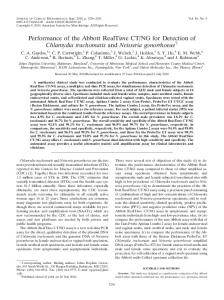
Figure 8. System reward as a function of task weight ratio for U=0.7, Ebudget =90%, and gain ratio =100 Figure 6 through Figure 8 shows the system reward R as a function of task weight ratio WR for U=0.7, gain ratio =100 and for Ebudget set to 30%, 60%, and 90% respectively. As it can be seen, LRD is the best performing heuristic throughout the spectrum, followed by LRSP. R increases roughly linearly with WR. When we keep U, gain ratio, and Ebudget constant and vary WR, we are effectively linearly rescaling wi for each task. As WR increases wi increases linearly which increases the overall system reward R. Moreover, as WR increases the range

1000 0 10

20

30

40 50 60 70 Weight Ratio (WR)

80

90

100

Figure 6. System reward as a function of task weight ratio for U=0.7, Ebudget=30%, and gain ratio =100 We generated 100,000 generic task sets and then for each task set, we changed the above parameters over the

4.8

over which wi varies increases which also makes the difference between the performances of heuristics more significant. On the other hand, as Ebudget increases the performance margin between the different heuristics diminishes because more deadlines can be met and the system reward becomes closer to its maximum possible value.

Figure 10. System reward as a function of total utilization for Ebudget=Ebound(U=0.3), WR=50, and gain ratio =100 Figure 10 shows R as a function of U for Ebudget=Ebound(U=0.3), gain ratio=100, and WR=50 for each heuristic. Unlike Figure 6 through Figure 9 where Ebudget is recalculated as a percentage of Ebound which is also a function of the total utilization U, in this set of experiments Ebudget is set to a fixed value, namely the energy required to meet all the deadlines when U=0.3 (i.e. Ebound(U=0.3) ). When U ≤ 0.3 the system has enough energy budget to meet all deadlines (i.e. Ebudget ≥ Ebound) and all the heuristics yield the same reward, which is simply the maximum possible system reward. As U increases from 0.3 to 1.0, R starts to decrease until it reaches its minimum value when U=1.0 and the differences in performance between the different heuristics become more significant. As U increases Ci increases linearly for each task while wi remains constant. Hence, as U increases, more energy has to be spent to execute the same number of jobs, (thus to get the same R), compared to a smaller value of U. Consequently, as U increases R decreases.

8000 7000 LRD

System Reward (R)

6000

LRSP

5000

LRDSP

4000

LRSU 3000

LR

2000

FSJ

1000 0 10

20

30 40 50 60 70 80 90 Energy Budget (% of Energy Bound)

100

Figure 9. System reward as a function of Ebudget for U=0.7, WR=50, and gain ratio =100

5000

Figure 9 shows the system reward R as a function of Ebudget for U=0.7, gain ratio=100 and WR=50 for each heuristic. Again, LRD outperforms other heuristics. When Ebudget is small, say 10%, the system is very energyconstrained and only a very small number of jobs can be executed. Under such conditions the difference in performance between the different heuristics is small. As Ebudget increases the system becomes less energy constrained: more task instances can be executed which increases the overall system reward and the difference between the heuristics becomes more significant. As Ebudget approaches 100%, the reward achieved by the different heuristics converge and they become exactly equal when Ebudget=100%, since in this case, the system has enough energy to meet all the deadlines and R reaches its maximum value.

System Reward (R)

4000

System Reward (R)

LRSU LR FSJ

2000 0.2

0.3

0.4

0.5

0.6

0.7

0.8

0.9

FSJ

10

25

50 75 Gain Ratio

100

500

1000

Figure 11 shows system reward R as a function of the logarithm of the ratio of normal-mode power to standbymode power (namely, log(gain ratio)) for U=0.7, Ebudget=30 and WR=50 for each heuristic. As gain ratio increases the standby-mode power consumption glow decreases and so does the idle energy. Consequently, there is more energy available to be used for executing jobs in the normal mode which increases the system reward. Hence, R increases with gain ratio. Note that Figure 11 shows a cut-off gain ratio of 50 beyond which the system reward remains practically constant. This is an important result since it shows that decreasing the stand-by power consumption beyond a certain threshold does not provide significant advantage. This behavior can be explained by noting that as gain ratio increases (as glow becomes very small) the increase in the available energy for normal mode

LRDSP

0.1

LR

Figure 11. System reward as a function of gain ratio for U=0.7, Ebudget=30%, and WR=50

LRSP

3000

LRSU

2000

5

LRD

4000

LRDSP

0

7000

5000

LRSP

3000

1000

8000

6000

LRD

1

Total Utilization (U)

4.9

becomes practically too small to be used for executing any additional jobs and the system reward saturates.

[10] D. Mosse, H. Aydin, B. Childers, and R. Melhem. Compiler-assisted dynamic power-aware scheduling for real-time applications. Workshop on Compilers and Operating Systems for Low-Power (COLP’00), 2001. [11] P. Pillai and K.G. Shin. Real-time dynamic voltage scaling for low power embedded operating systems. Symposium on operating systems principles, pages 89102, 2001. [12] G. Quan and X. Hu. Energy efficient fixed-priority scheduling for real-time systems on variable voltage processors. Design Automation Conference, pages 828-833, 2001. [13] C. Rusu, R. Melhem and D. Mosse. Maximizing the system value while satisfying time and energy constraints. Real-Time Systems Symposium, pages 246 -255, 2002. [14] Y. Shin and K. Choi. Power conscious fixed priority scheduling for hard real-time systems. Design Automation Conference, pages 134–139, 1999. [15] Y. Shin, S. Lee and J. Kim. Intra-task voltage scheduling for low-energy hard real-time applications. IEEE Design and Test of Computers, 18(2): 20-30, 2001. [16] F. Yao, A. Demers, and S. Shenker. A scheduling model for reduced cpu energy. IEEE Annual Foundations of Computer Science, pages 374–382, 1995.

6. CONCLUSION In this paper, we proposed a generic performance optimization framework for energy-constrained real-time operating systems. Our approach entails selecting jobs for execution to maximize the number of met deadlines, or alternatively maximize the reward (utility) of the system. We presented an optimal algorithm FSJ that achieves the first objective in time O(n log n), where n is the number of tasks. We proved that achieving the second objective is NP-Hard. We proposed some fast heuristics for this problem and presented experimental results that showed the relative performance of these heuristics. The best performing heuristic is LRD which favors tasks with higher wi/Ci ratio, which represents the reward return per unit energy spent in executing a task.

REFERENCES [1] H. Aydin, R. Melhem, D. Mosse and P.M. Alvarez. Determining optimal processor speeds for periodic real-time tasks with different power characteristics. Proceedings of the 13th EuroMicro Conference on Real-Time Systems (ECRTS’01), pages 225-232, 2001. [2] H. Aydin, R. Melhem, D. Mosse and P.M. Alvarez. Dynamic and aggressive scheduling techniques for power-aware real-time systems. Proceedings of the 22nd Real-Time Systems Symposium (RTSS’01), pages 95-105, 2001. [3] H. Aydin and Q. Yang. Energy-aware partitioning for multiprocessor real-time systems. Proceedings of the 17th International Parallel and Distributed Processing Symposium (IPDPS’03), Workshop on Parallel and Distributed Real-Time Systems, 2003. [4] M.R. Garey and D.S. Johnson. Computers and Intractability: A Guide to the Theory of NPCompleteness. Freeman, 1979. [5] M. Hamdaoui and P. Ramanathan. A dynamic priority assignment technique for streams with (m,k)-firm deadlines. IEEE Trans. Computers, 44(12): 1995. [6] P. Kumar and M. Srivastava. Power-aware multimedia systems using run-time prediction. International Conference on Computer Design, pages 64-69, 2001. [7] C.L. Liu, J.W. Layland. Scheduling algorithms for multiprogramming in a hard-real time environment, Journal of the ACM, 17(2). 1973. [8] J. Liu. Real-Time Systems. Prentice Hall, NJ, 2000. [9] J. Liu, P.H. Chou, N. Bagherzadeh, and F. Kurdahi. Power-aware scheduling under timing constraints for Design mission-critical embedded systems. Automation Conference, pages 840-845, 2001.

4.10