COVER FEATURE
Energy-Efficient Area Monitoring for Sensor Networks The nodes in sensor networks must self-organize to monitor the target area as long as possible. Optimizing energy consumption in area coverage, request broadcasting, and data aggregation can significantly extend network life.
Jean Carle David Simplot-Ryl University of Lille
40
R
ecent advances in microelectromechanical systems, digital electronics, and wireless communications have enabled the development of low-cost, low-power, multifunctional sensor devices. These devices can operate autonomously to gather, process, and communicate information about their environments. When a large number of devices collaborate using wireless communications and an asymmetric, many-to-one data flow, they constitute a sensor network.1 The sensor nodes usually send their data to a specific sink node or monitoring station for collection. If all the nodes communicated directly with the monitoring station, the communication load— especially over long distances—would quickly drain the network’s power resources. Therefore, the sensors operate in a self-organized, decentralized manner that maintains the best connectivity as long as possible and communicates messages via multihop spreading. Sensor networks are a special case of ad hoc networks. Figure 1 shows two kinds of applications. In event-driven applications like forest-fire detection, one or several sensor nodes detect an event and report it to a monitoring station. In demanddriven applications like inventory tracking in a factory warehouse, sensors remain silent until they receive a request from the monitoring station. In both cases, sensor networks generally deploy nodes densely, using hundreds or thousands of sensors— placed mostly at random—either very near or inside the phenomenon to be studied. The nodes are sta-
Computer
tic and carry less battery and processing power than standard ad hoc networks. A sensor’s battery is not replaceable, so its energy is the most important system resource—especially when the network operates in hostile or remote environments. The best method for conserving energy is to put as many sensors to sleep as possible. At the same time, however, the network must maintain its functionality through a connected subnetwork that lets the monitoring station communicate with any of the network’s active sensors. Our group at the Fundamental Computer Science Laboratory of Lille (LIFL) is developing strategies for selecting and updating an energy-efficient connected active sensor set that extends the network lifetime. We report optimizing solutions to three separate problems: • area coverage—maintaining full coverage of the monitoring area; • request spreading—broadcasting from the monitoring station to the covering nodes; and • data aggregation—transmitting information from nodes to the monitoring center. Each sensor’s monitoring area can be approximated as a disk around the sensor. We further assume that each sensor can measure or observe the physical parameter or event in its own monitoring area and can use radio-frequency technology to communicate with other sensors in its vicinity. The solutions we present here also assume that a sensor’s monitoring area is exactly the same as its commu-
Published by the IEEE Computer Society
0018-9162/04/$20.00 © 2004 IEEE
Sensing area
1. Request using flooding
Report
Event 3. Report Report
Monitored area
Monitoring station (sink)
Monitoring station (sink)
(a)
nication area—that is, the area in which nodes can receive communication from a transmitting node.
(b)
Monitored area
2. Report using multihop and tree structure
which could involve significant communication overhead once sensors start to die between activity periods.
Figure 1. Sensor network applications. (a) In event-driven applications, one or several sensors detect an event and report it to a monitoring station. (b) In demand-driven applications, sensors remain silent until they receive a request from the monitoring station.
AREA COVERAGE Consider a sensor node set dropped randomly on a target area that it must monitor. The monitored area is the union of all individual node monitoring areas. Assuming that the sensing radius of each node is the same and that the sensors can obtain their geographical position, solving the areacoverage problem requires finding the area-dominating set—that is, the smallest subset of sensor nodes that covers the monitored area. Nodes not belonging to this set do not participate in the monitoring—they sleep. The area-dominating set changes periodically both as a function of activity scheduling and to extend the network’s monitoring capability. Recently, Fan Ye and colleagues2 proposed a simple localized protocol for dynamically selecting an area-dominating set. According to this protocol, a node sleeps for a while and then decides to be active if and only if there are no active nodes closer than a given threshold distance from it. When a node is active, it remains active until the end of its battery lifetime. Sleeping nodes periodically reevaluate their decision. With this protocol, the probability of having full coverage of a monitored area is close to 1 if the threshold is less than 1/(1 + √5) of the sensing area’s radius. However, this protocol has limited usefulness because it is probabilistic and does not ensure full area coverage. Di Tian and Nicolas D. Georganas3 proposed a solution that requires every node to know all its neighbors’ positions before making its monitoring decisions. Each node then selects a timeout interval. At the end of the interval, if a node sees that neighbors who have not yet sent any messages together cover its monitoring area, the node transmits a “withdrawal” message to all its neighbors and goes into sleep mode. Otherwise, the node remains active but does not transmit any message. The process repeats periodically to allow for changes in monitoring status. The problem with this solution is that it requires a priori knowledge about all neighboring sensors,
Dominating node sets We have developed solutions to the area-coverage problem that guarantee coverage—as long as the given sensor nodes cover the area—without requiring nodes to have prior knowledge of neighboring nodes. Instead of covering an area, the goal is to select a connected dominating set of sensor nodes that “monitor” other sensors within their coverage range, or neighborhood. Researchers have studied this problem in the context of ad hoc network broadcasting.4 A dominating set is a subset of network nodes in which each node is either in this subset or is a neighbor of a node in this subset. A dominating set is connected if any two nodes in the set can communicate, possibly through other nodes via multihop broadcasting. The broadcasting task is to send a message from one node to all network nodes using only nodes in a connected dominating set. Among recently developed strategies for constructing small connected dominating sets, localized protocols offer the best prospect for achieving energy efficiency. In a localized protocol, each node makes decisions based solely on information about itself and its one-hop neighbor—if position information is also available—or its two-hop neighbors—if position information is not available. Moreover, each node makes decisions without communications between nodes beyond the message exchanges that nodes use to discover each other and establish neighborhood information. The local information must suffice for a node to decide whether or not it is in a connected dominating set; otherwise, the increased communication overhead could offset the energy savings. Recently, Fai Dai and Jie Wu5 proposed a distributed dominant-pruning algorithm to meet these solution criteria. This algorithm gives each node a priority, which can be simply its unique identifier or a combination of remaining battery life, number of neighbors, and identifier. February 2004
41
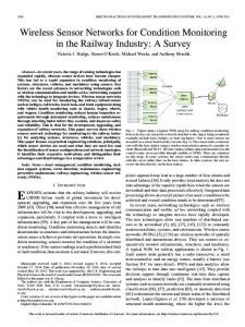
Figure 2. Dominantpruning algorithm. A node belongs to the dominating set if and only if no subset fully covers it.
1
Nongateway node Gateway node
6 8 2
10 7
9
3
5 4
A node u is “fully covered” by a subset S of its neighboring nodes if and only if three conditions hold: • the subset S is connected, • any neighbor of u is a neighbor of at least one node from S, and • all nodes in S have higher priority than u. A node belongs to the dominating set if and only if no subset fully covers it. The nodes belonging to a dominating set are gateway nodes; other nodes are nongateway nodes. For instance, Figure 2 shows a graph that uses the node identifier for priority. For node 1, S = {6}, so node 6 fully covers node 1; consequently, node 1 is a nongateway node. For node 6, S = {8}, but node 1 is not a neighbor of node 8; therefore, node 6 is a gateway node. For node 7, S = {8, 9, 10} and its additional neighbors, nodes 3, 4, and 5, are neighbors of nodes 10, 9, and 9, respectively; therefore, node 7 is covered by its set S and is a nongateway node. For node 10, the corresponding set S is empty; therefore, 10 is a gateway node because its neighbors have no node in S to satisfy the second condition. Note that this definition allows each node to decide about its dominating node status without requiring a message exchange. The knowledge of either its two-hop neighbors or its one-hop neighbors with their geographic positions is sufficient. Each node can decide whether or not it is a gateway node by running the following procedure: • collect information about neighborhood and neighbor priorities; • compute subgraph of one-hop neighbors with higher priority; • if this subgraph is connected and if each onehop neighbor is either in this subgraph or the neighbor of at least one node in this subgraph, the node chooses nongateway status; otherwise, the node chooses gateway status. Dai and Wu’s original algorithm5 defined priority by node identifiers, leaving the energy remaining in non42
Computer
gateway nodes available for extending network life. A variation of the dominating-set protocol uses timeouts to transmit selected priorities to a vicinity. At the beginning of the process, each node selects a timeout that is inversely proportional to the node’s priority (the timeout function may also depend on a random variable). This means that a node with high priority selects a short timeout and vice versa. At the end of this waiting period, the node can indicate its priority by broadcasting its identifier to its neighbors. The node can also transmit its gateway decision at the same time. Thus, at the end of the waiting period, each node knows which of its neighbors have higher priority and are gateway nodes.
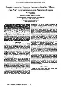
Area-dominating sets We can use this information to modify the dominating-set protocol to find area coverage rather than node coverage. In this modification, each node computes its timeout function based on its priority and listens to messages from other nodes before deciding its dominating status at the end of a timeout interval. A node choosing gateway status always transmits a message (positive advertising) to all its neighbors. A node choosing not to monitor its area has the option of transmitting this information to its neighbors (negative advertising) or not. The protocol runs as follows: • using a simple perimeter coverage scheme,3 node A computes the area covered by each node that transmits either positive or negative advertising and includes the transmitting node in a subset; • at the end of its timeout interval, node A computes a subgraph of its one-hop neighbors that sent advertisements (these are its neighbors with higher priority); • if this subgraph is connected and if the subgraph nodes fully cover node A’s area, node A opts for nongateway (sleeping) status; otherwise, the node chooses gateway (active) status. Figure 3 shows the possible decision results at a central node A based on different information available through positive-only advertising and through positive and negative advertising. The distributed dominant-pruning algorithm can prove that this area-dominating set is connected. In the case of positive-only advertising, each node simply ignores nodes that remain silent and inactive. In the positive-and-negative-advertising case, a node gives higher priority to all nodes with pre-
Inactive
(a)
Active
(b)
vious advertisements and treats them as part of a subset that must be connected. In both cases, the proof is similar to the connectivity proof given for the dominant-pruning algorithm. It suffices here to set the priority in Dai and Wu’s algorithm to the remaining battery life. Let G be the area-dominating set that the algorithm generates, and let F be the dominating set of G that the dominant-pruning protocol generates. If the monitoring area of a node u is covered by a connected subset of its neighbors with more battery life—that is, shorter timeout and therefore higher priority—the set of neighbors of u is “fully covered” by this same subset. In other words, if a node does not belong to G, it also does not belong to F. Hence, the area-dominating set G includes the constructed dominating set (of neighbors) F. Since F is proven to be connected, it follows that G is also connected. This property of a connected area-dominating set is important for request propagation and collection of sensor replies. Figure 4 shows how negative advertising can reduce the number of active sensors and therefore prolong network life. Numbers represent timeouts. Nodes 0, 1, 2, 3, and 4 announce their activation. Node 5 decides to be inactive since previously advertised nodes are connected and cover its monitoring area. If node 5 does not announce its deactivation, node 6 decides to be active because it does not know that the area A is covered. If node 5 announces its status, node 6 decides to be inactive because the negative advertising also brings information about coverage—that other nodes with shorter timeouts cover node 5’s sensing area. The network can reselect covering nodes periodically to spread the sensing cost dynamically over all nodes in a fair manner. This method significantly extends the network’s life. If the density is more than 30 nodes per unit area, the area-dominating graph is sparse, with nodes having on average three neighbors. In addition, the distance between its two neighboring nodes is typically two-thirds of the transmission radius. Hence, active nodes form a
(c)
very simple network with a structure similar to regular hexagonal tiling.
REQUEST SPREADING Wireless ad hoc networks commonly use broadcasting to find routes and to disseminate requests and data, and many research efforts have addressed the design of energy-efficient broadcast protocols.4 The protocols differ for nodes with fixed transmission ranges and those that can adjust their transmission ranges.
Fixed transmission ranges
Figure 3. Examples of configurations in which the central node, which is in its default inactive state, makes its area-coverage decision. (a) Central node decides to be active because its active neighbors do not fully cover its monitoring area; (b) central node decides to remain inactive because its monitoring area is covered by active neighbors that are connected; and (c) central node decides to be active because the active neighbors that cover its monitoring area are not connected.
When all nodes have a fixed transmission radius, the basic broadcast protocol is blind flooding: A sequence number identifies each broadcast message, and a node receiving the message for the first time retransmits it to its neighbors. In general, blind flooding generates redundant transmissions and leads to many packet collisions in the media access control (MAC) network layer. But in the sparse and uniformly distributed networks of area-dominant nodes that we have defined for area coverage, blind flooding produces a satisfactory solution. Researchers have proposed several protocols to minimize retransmissions while trying to guarantee that every node receives a broadcast message.4 Dai and Wu’s dominant-pruning algorithm5 is one. Figure 4. Negative advertising. Node 6 can exhibit different behaviors depending on whether or not node 5 advertises its decision to be inactive.
2
1 6
5 3
0 4 A
February 2004
43
Figure 5. Sensor networks with dominating set applied over areadominating set. (a) Original network with areadominating set (black nodes), and (b) dominating set of neighbors applied over areadominating set.
(a)
Applying it to the area-dominating set reduces the number of retransmissions with respect to blind flooding on the order of 20 percent, with most of the savings coming from sensors along the border of the monitored area. The dominant-pruning method is easy to apply since the dominating-set information is already available from constructing the area-dominating set. Figure 5 illustrates a sensor network with its area-dominating set and its dominating set used for broadcasting. Forwarding-neighbor protocols also can minimize retransmission requirements. In this approach, each network node has a relay subset composed of neighbor nodes. When a node transmits a broadcast packet, only nodes in its relay subset will consider forwarding the message. The multipoint relay protocol6 is a deterministic method for reliable broadcasting in this context. The MPR algorithm selects a minimal set of one-hop neighbors that cover the same network as the complete set of neighbors. MPR is a greedy algorithm because computing the minimal set is an NP-complete problem. MPR is also an explicit broadcast protocol since each node finds its relay set by repeatedly adding the (one-hop) neighboring nodes until the relay subset constitutes the maximum possible neighbors not yet covered. Broadcasting is source dependent and may exclude nodes that received the same message as the relay node from consideration for relay node decisions. The list of relay nodes is attached to the retransmitted packet. When applied on the areadominating sets, MPR constructs relay subsets that contain nearly all nodes. Thus there is no advantage to applying MPR to area-dominating sets. A proposed variant of MPR dedicated to sensor networks replaces the number of noncovered neighbors measured in the greedy algorithm.7 Instead, it uses a “utility function” that multiplies the num44
Computer
(b)
ber of noncovered neighbors with a function of the remaining battery power.
Adjustable transmission ranges Fixed-transmission-range protocols aim to save energy by reducing the number of sensors that participate in broadcasting. Adjustable-transmissionrange protocols measure energy savings differently. The energy consumption for a unit message sent distance r is measured as rα + c, where α is a signal attenuation constant greater than 2 and c is a positive constant that represents c signal processing, minimum energy needed for successful reception, and c MAC-layer control messages.8 An energy-efficient solution using this method may require more nodes to reach every node than a fixed-transmission solution requires, but each node may expend less energy. Thus, control of the emitted transmission power can significantly reduce energy consumption and so increase the network’s lifetime. However, adjusting the transmission signal strength generally implies topology alterations that lose connectivity. Hence, nodes must manage their transmission area while maintaining network connectivity. To preserve connectivity and obtain full coverage of awake sensors, the main topology-control challenge is to design localized algorithms for deciding which edges are necessary for global connectivity. For instance, a relative neighborhood graph (RNG) is a locally defined subgraph that removes an edge between two nodes u and v if a node w is closer to u and v than the distance between u and v. As Figure 6 shows, this RNG subgraph contains the original graph’s minimum spanning tree, which is defined in a globalized manner. Ning Li, Jennifer C. Hou, and Lui Sha9 recently proposed a local version of MST that preserves connectivity. To define the local MST, each node computes the MST over its one-hop neighborhood and retains only the
(a)
(b)
(c)
(d)
(a)
neighbors in this subgraph. Thus, only edges that two endpoints choose remain in the graph. MST is a subset of LMST—an edge that belongs to MST also belongs to the LMST graph. LMST is a subset of RNG.10 Hence, LMST is the bestknown local approximation of globalized MST. Since the MST subgraph is connected if the original graph is connected, LMST and RNG subgraphs that contain MST are also connected. Hence, a topology-control algorithm that preserves LMST edges guarantees network connectivity. Other LIFL research has proposed adaptive protocols that use RNG or LMST subgraphs to ensure connectivity conservation.10,11 In this work, each node’s transmission radius is chosen to reach nonattained RNG or LMST neighbors. Although minimizing the transmission range is not always optimal (except for c = 0), it is possible to determine an opti-
Figure 6. Proximity graphs. (a) Unit graph, (b) minimum spanning tree, (c) relative neighborhood graph, and (d) local MST (100 nodes with average degree of 14).
(b)
mal radius for power-efficient broadcasting either experimentally or theoretically. In broadcasting requests over area-dominating sets, the regularity of the created topology limits transmission power choices. Indeed, as Figure 7a shows, the degree of an area-dominant node is about 3 and the number of LMST neighbors is around 2. When an area-dominant node receives a request message, usually only one LMST neighbor has not yet received it. This reduces the transmission radius by about 30 percent since the average distance between two area-dominant nodes is about two-thirds of maximal radius. For an energy model with α = 2 and c = 0, the energy savings for a single broadcast is about 65 percent, given the reductions in communication power requirements and LMST leafs that must resend the request.
Figure 7. LMST algorithm. (a) Applying the LMST algorithm over an area-dominating set illustrates the simplicity of the obtained graph: Nodes only need to take care of two or three neighbors. (b) Spanning tree induced by flooding over an areadominating set starting from the monitoring station. A node that receives the broadcast message for the first time considers the sender of the message as its parent in the distributed spanning tree.
February 2004
45
DATA AGGREGATION After a sensor node receives a request, it must respond by reporting its measurements. Aggregating sensor measurements to report only important information, such as average or extreme values, can further reduce energy consumption. For instance, a surveillance application can request that the sensors count the number of sites that observe a temperature greater than a given threshold. One technique for limiting the number of reply messages uses the spanning tree induced by flooding during request spreading.7 Figure 7b shows this spanning tree for the same initial graph shown in Figure 5. Following construction of the tree, the parent nodes transmit data coming from multiple sensor nodes to the monitoring station via their own parent. For particular requests, such as inventory, a node can wait to have multiple replies from all its successors in the tree before replying with data fusion—sending the sum of its successors’ replies instead of retransmitting all replies. This solves implosion and overlap problems.
n future work, we plan to study sensor networks in which the sensing and transmission radii are different. In fact, the existence of an optimal transmission radius in the request-spreading process suggests an advantage in having a transmission radius larger than the sensing radius because the sensing radius directly affects the average distance between area-dominant nodes. Moreover, enlarging the transmission radius can also benefit data-fusion schemes by allowing the construction of better-balanced trees. ■
I
References 1. I.F. Akyildiz et al., “Wireless Sensor Networks: A Survey,” Computer Networks, vol. 38, 2002, pp. 393422. 2. F. Ye et al., “PEAS: A Robust Energy Conserving Protocol for Long-Lived Sensor Networks,” Proc. IEEE Int’l Conf. Network Protocols (ICNP 2002), IEEE CS Press, 2002, pp. 200-201. 3. D. Tian and N.D. Georganas, “A Coverage-Preserving Node Scheduling Scheme for Large Wireless Sensor Networks,” Proc. 1st ACM Workshop Wireless Sensor Networks and Applications, ACM Press, 2002; pp. 32-41. 4. I. Stojmenovic and J. Wu, “Broadcasting and Activity-Scheduling in Ad Hoc Networks,” to be published in Ad Hoc Networking, S. Basagni et al., eds., IEEE Press, 2004.
46
Computer
5. F. Dai and J. Wu, “Distributed Dominant Pruning in Ad Hoc Networks,” Proc. IEEE 2003 Int’l Conf. Communications (ICC 2003), IEEE Press, 2003, pp. 353-357. 6. A. Qayyum, L. Viennot, and A. Laouiti, “Multipoint Relaying for Flooding Broadcast Messages in Mobile Wireless Networks,” Proc. 35th Ann. Hawaii Int’l Conf. System Sciences (HICSS-35), IEEE CS Press, 2002, pp. 298-307. 7. J. Lipman et al., “Resource Aware Information Collection (RAIC) in Ad Hoc Networks,” Proc. 2nd Mediterranean Ad Hoc Networking Workshop (MED-HOC-NET 2003), 2003, pp. 161-168. 8. L.M. Feeney, “An Energy-Consumption Model for Performance Analysis of Routing Protocols for Mobile Ad Hoc Networks,” ACM J. Mobile Networks and Applications, vol. 3, no. 6, 2001, pp. 239249. 9. N. Li, J.C. Hou, and L. Sha, “Design and Analysis of an MST-Based Topology Control Algorithm,” Proc. IEEE Infocom 2003, IEEE Press, 2003, pp. 17021712. 10. J. Cartigny et al., “Localized LMST and RNG-Based Minimum-Energy Broadcast Protocols in Ad-Hoc Networks,” to be published in Ad Hoc Networks, 2004. 11. J. Cartigny, D. Simplot, and I. Stojmenovic, “Localized Minimum-Energy Broadcasting in Ad-Hoc Networks,” Proc. IEEE Infocom 2003, IEEE Press, 2003, pp. 2210-2217.
Jean Carle is an associate professor in the Fundamental Computer Science Laboratory of Lille (LIFL) at the University of Lille, France. His research interests include distributed computing, data communication, mobile ad hoc networks, and sensor networks. Carle received a PhD in computer science from the University of Amiens. Contact him at
[email protected].
David Simplot-Ryl is an associate professor in LIFL at the University of Lille. His research interests include ad hoc networks, distributed computing, embedded operating systems, and RFID technologies. Simplot-Ryl received a PhD in computer science from the University of Lille. Contact him at
[email protected].