Energy-Efficient Continuous Activity Recognition on Mobile Phones: An Activity-Adaptive Approach Zhixian Yan1 , Vigneshwaran Subbaraju2 , Dipanjan Chakraborty3 , Archan Misra2 , Karl Aberer1 1
EPFL Switzerland {zhixian.yan, karl.aberer}@epfl.ch
2
3 Singapore Management University IBM Research Lab Singapore India {vigneshwaran, archanm}@smu.edu.sg∗
[email protected]
Abstract
multiple body-worn accelerometer sensors [4, 13], for improved activity recognition accuracy. As prior studies (e.g., [6, 9]) have demonstrated that continuous activity recognition (applying on-board data processing over accelerometer and other sensor data streams) can rapidly drain the power on mobile devices, it is important to reduce the energy overheads of continuous mobile sensing [8, 12, 14]. Accordingly, our work addresses the problem of developing an energy-efficient, continuous approach for accelerometer-based recognition of locomotive and postural activities, using a mobile device-embedded accelerometer sensor. Specifically, we focus on two independent parameters of the accelerometer-based activity recognition process: a) the sensor sampling frequency and b) the set and classes of features used in activity classification. Investigations (e.g., [5]) have established that these two parameters jointly influence a tradeoff between two important and mutually-conflicting objectives: 1) increase classification accuracy: Increase in sampling frequency and a richer set of features both result in improved activity classification accuracy; 2) reduce energy overheads: Conversely, reducing the sampling frequency, duty cycle and/or the set of features help to lower the energy overhead. To reduce the energy overheads of accelerometer-based activity recognition, we first study the combined influence of these two parameters on the recognition accuracy, separately for each distinct activity. We find that different activities indeed differ in how their classification accuracy varies with changes to the sampling frequency and the set of classification features used. We also study how the recognitionrelated energy overhead on commercial smartphones varies with these two parameters. Taken together, these studies help establish that the most judicious combination of (sampling frequency, classification feature) used for activity recognition is different for each distinct activity. This observation marks an important point of departure from earlier work, which has largely focused on adapting either the sensor selection (among multiple sensors) or the sensing duty cycle [14] in an activity-oblivious fashion.
Power consumption on mobile phones is a painful obstacle towards adoption of continuous sensing driven applications, e.g., continuously inferring individual’s locomotive activities (such as ‘sit’, ‘stand’ or ‘walk’) using the embedded accelerometer sensor. To reduce the energy overhead of such continuous activity sensing, we first investigate how the choice of accelerometer sampling frequency & classification features affects, separately for each activity, the “energy overhead” vs. “classification accuracy” tradeoff. We find that such tradeoff is activity specific. Based on this finding, we introduce an activity-sensitive strategy (dubbed “A3R” – Adaptive Accelerometer-based Activity Recognition) for continuous activity recognition, where the choice of both the accelerometer sampling frequency and the classification features are adapted in real-time, as an individual performs daily lifestyle-based activities. We evaluate the performance of A3R using longitudinal, multi-day observations of continuous activity traces. We also implement A3R for the Android platform and carry out evaluation of energy savings. We show that our strategy can achieve an energy savings of 50% under ideal conditions. For users running the A3R application on their Android phones, we achieve an overall energy savings of 20-25%.
1
Introduction
Accelerometers are one of the most common sensors on smartphones, and have been widely used in the mobile sensing literature to ascertain an individual’s locomotive or postural behavior (e.g., sitting, standing, cycling or climbing steps). The vast majority of literature on accelerometerdriven activity sensing focuses on either a) the use of progressively more sophisticated features [16] or b) the use of ∗ V.
Subbaraju and A. Misra’s research is supported by the Singapore National Research Foundation under its International Research Center@Singapore Funding initiative and administered by the IDM Program Office.
1
Based on our observation, we develop an adaptive accelerometer activity recognition (A3R) approach for continuous activity recognition. The central idea behind A3R is to continually track the current/ongoing activity of the user, and then dynamically adjust the two parameters (sampling frequency, classification features) to a choice that is ‘optimal’ for this activity. A3R exploits the fact that an individual’s daily lifestyle typically consists of a sequence of moderately-long lasting activities, and that many (but not all) of these commonplace activities (such as sitting or standing) can be classified quite accurately, without requiring sophisticated features or high sampling rates. It is worth stating that A3R is designed for monitoring the salient daily lifestyle activities and is not intended for capturing ephemeral gestures or transient, jerky movements. We also address the question of how much energy savings A3R can achieve in practice, as users engage in their normal daily lifestyle, leading to individualized variations in the frequency and relative duration of the different activities. We collect and analyze longitudinal data traces about the variation in smartphone-based accelerometer readings of multiple subjects, under naturalistic and daily lifestyledriven usage of the phone, to help quantify the energy savings that may be achieved by A3R. We also utilize an Android-based implementation of A3R to perform in-situ studies and empirically establish that A3R is able to mitigate the energy burden of continuous activity recognition. User Studies and Datasets: To validate, and quantify the performance impact of the A3R approach, we utilize two different user-generated datasets (detailed further in Sections 3.2 and Section 5): • Short Training Data, Annotated with Ground Truth: To research the energy vs. accuracy tradeoffs for different activities, we had 4 users each engage in a pre-defined sequence of specified activities for relatively short durations (5 mins per activity), providing us a groundtruth annotated, multi-person dataset. • Long Natural-Lifestyle Data, without Ground Truth: To understand the A3R under naturalistic lifestyledriven activity sequences, we employed two different data sets. The first data set continuously captured the accelerometer data from the phones of 6 users, over a period of 6-8 weeks. We use this to evaluate A3R’s energy savings potential in emulated settings. In another study, we monitored the battery drainage profile for 2 users engaged in their everyday lifestyle activities while A3R was running on their Android phones, helping us to observe whether A3R makes any meaningful difference in smartphone operational lifetime, given their regular usage patterns. The rest of the paper is organized as follows. Section 2 presents related work on accelerometer-based activ-
ity recognition. Section 3 then studies the impact of varying the sensor sampling frequency and the choice of classification features on the per-activity classification accuracy and the smartphone energy consumption. Section 4 then presents the A3R approach, while Section 5 then presents our dataset-driven empirical results. Finally, Section 6 concludes the paper.
2
Related & Background Work
Early research on the use of individual or multiple body-mounted accelerometers for locomotive activity sensing focused on understanding the various factors affecting the recognition accuracy–e.g., [3] demonstrated that different activities exhibited differing levels of classification accuracy, depending on the on-body placement of the accelerometers. The impact of sampling rate on classification accuracy & power was studied for the eWatch platform in [6], where the mean of the signal was used as the classification feature. For the platform-specific accelerometers studied, they observed no differential impact on battery lifetime between the use of time vs. frequency domain features. This turns out to be not the case for our Android phones. [6] also described multiple selective sampling strategies based on a Markovian model of transitions between different activities. Similarly, [5] also studied the impact of sampling rate (& signal resolution) on classification accuracy, whereas [1] studied the classification accuracy based on multiple body-worn accelerometers, as a function of a more complex set of both time & frequency domain features (such as mean, energy and entropy). [13] showed how classification accuracy could be improved by using meta-level classifiers, such as feature boosting and MDTs. Most of these results do not directly apply to a commercial smartphone device (for example, a phone’s background energy consumption is significantly higher than a custom-built sensor). More recently, the use of a secondary sensing ‘co-processor’ has been shown [10][7]) to provide highly energy-efficient activity recognition on mobile devices; such hardware-based optimizations are complementary to our focus on optimizing the computational logic of activity sensing. More recently, adaptive online techniques have been proposed to reduce the energy overheads specifically associated with personal mobile devices. One possible approach is smart duty-cycling. The EEEMS hierarchical framework [14] for smartphones turns on more power-expensive sensors (such as GPS) only when less energy-hungry sensors (such as accelerometer) detect a significant event. Similarly, [14] also duty-cycles the accelerometer (at approx. 50%) to reduce its energy overhead. The Kobe toolkit [2] focuses on balancing the accuracy and energy cost of activity classification algorithms on mobile devices, by dynam-
3
Characterizing the Classification Accuracy vs. Energy Consumption Tradeoff
Prior work on accelerometer-based classification has principally focused on identifying the key features that enable the most accurate identification of different locomotive/postural states. Table 1 lists some of the commonlyused features, which can be broadly classified into two categories (Ftime and Ff req ). More detailed accelerometer features can be referred to [15]. • Time-domain Features (Ftime ): These features are computed directly on the appropriate frames (e.g., 5sec, 10sec) of accelerometer streams; examples include the variance/mean of the frame as well as twoaxis correlations. • Frequency-domain Features (Ff req ): Here, features such as entropy & energy are computed over frequency domain coefficients, which are first obtained by using FFT (or alternatives, such as wavelets) on each frame. In either case, it is important to observe that the features are currently applied in an activity-independent fashion–i.e., the same set of features are used across all locomotive/postural states of the individual. Our fundamental hypothesis is that such an activity-independent use of features may not be the optimal–more specifically, different activities may be classified, with no or little loss in classification accuracy, by using different combinations of the haccelerometer sampling frequency, classification featuresi tuple. The advantage is that the use of a lower sampling frequency, or the computation of a smaller set of features, should impose a lower sensing & computational energy overhead, respectively. To verify this hypothesis, we next report on the energy overheads and the classification accuracy for different
Table 1: Selected features used for activity recognition p Mean (¯ x, y¯, z¯), Magnitude ( x2 + y 2 + z 2 ), Variance {var(x), var(y), var(z)}, Covariance {cov(x, y), cov(y, z), cov(x, z)},
Time Domain
(m2 )
PN
EnergyP ( j=1N j ), mj is FFT component Entropy (− n j=1 (pj ∗ log(pj )), pj is FFT histogram
Frequency Domain
combinations of sampling frequency (SF ) and classification feature (CF ), i.e., the hSF, CF i tuples.
3.1
The Energy Overhead
While we expect the classification accuracy to be activity-dependent, the energy overhead should be activityindependent. Accordingly, we first study the dependency of the energy overhead on the combination of sampling frequency and the types of features computed–i.e., the tuple hSF, CF i, on commercially available smartphones. Instead of trying out every possible combination of the individual features listed in Table 1, we simply consider the choice of using (i) all time-domain features, (ii) all frequency-domain features or (iii) all the time+frequency domain features. This is driven by our empirical observation that the major difference in energy consumption arises from a choice of using none vs. any of the domain-specific features; the exclusion or inclusion of a specific frequency (or time) domain feature has only a marginal effect. Fig. 1 plot the energy consumption (in Joules) over a 2hour period, for different hSF, CF i combinations, for our representative phone: the Samsung Galaxy S2, which supports sampling frequencies up to 100 Hz. Note that Android APIs only permit the sampling frequency to be adjusted between 4 discrete values ([5Hz, 16Hz, 50Hz, 100Hz] for our device. To obtain the readings, we powered off the network interfaces and the display, and used the PowerTutor utility to measure the energy consumption.1 We can easily make the following observations: 500
Samsung Galaxy S2 400
Energy Cost (Joules)
ically adjusting the pipeline of sampling frequency, feature extraction and machine learning components. The runtime adaptation, however, focuses principally on adjusting where the computation is executed (device. vs. cloud), in response to system changes (such as changes in phone battery levels or foreground processing load). In contrast, A3R focuses on selecting a profile much more dynamically, based on the changes in the user’s activity; A3R may be an add-on to the Kobe framework. Similarly, the SociableSense system [11] applies reinforcement learning techniques to adjust the duty cycle of multiple sensors and uses a multi-criteria decision theory to distribute the computational tasks between a mobile device and the cloud. SociableSense makes a binary decision (‘should I sense or not’?), based on information in prior sensing cycles; in particular, it adapts the accelerometer duty cycle based on whether the sensor has detected a movement or not – only two states, while A3R’s adaptive choices are based on a set of specific locomotive activities.
300
200
100
T−Domain + F−domain Only T−Domain 0
10
20
30
40
50
60
70
80
90
100
Sampling Frequency (Hz)
Figure 1: Energy consumption for the Samsung Galaxy S2 at different hSF, CF i combinations 1) The total energy overhead in continuous activity recognition clearly increases with sampling frequency. 1 Although not plotted here due to space limitations, we observed similar trends on the HTC Nexus 1, which supports sampling only up to 25Hz.
2) The increase in energy-overhead is non-linear. More importantly, the additional energy overhead incurred by including frequency-domain features is not constant, but in fact, a non-linear, logarithmic function of the sampling frequency. This is due to the O(nlogn) computational complexity (where n is the number of samples for a given frame) of the required FFT operation. The figure effectively illustrated the possibility of smart and non-intuitive tradeoffs between sampling frequency and features–for example, it is less expensive to utilize purely time-domain features at 50Hz vs. using a combination of time+ frequency domain features at 16Hz.
3.2
The Classification Accuracy
We now investigate the impact that different combinations in the (SF , CF ) domain have on the accuracy of activity recognition. We study 10 specific activities (i.e., stand, slowWalk, sitRelax, sit, normalWalk, escalatorUp, escalatorDown, elevatorUp, elevatorDown, downStairs). To perform this study, we had a total of 4 subjects perform each of the activities for a period of 5 minutes, resulting in a per-subject experimentation duration of 50 minutes for 10 activities. The features of all the individual activities are then provided (on a per-individual basis) as input to a classifier (we used the J48 adaptive decision tree classifier in the Weka toolkit) to build a classification model that is customized to each test subject. The classification accuracy is then gauged by running a 10-fold cross validation on the data, at different sampling frequencies and for different feature combinations. Note that the classifier training was performed at the ‘maximum’ sampling frequency of 100 Hz, while the validation experiments utilized the appropriately varying sampling frequency. We have verified that performing the classification/learning at the same sampling frequency as the actual test frequency has only minimal effect on the observed classification accuracy. Accordingly, for on-phone deployments, as the training phase may be considered to be a onetime, offline activity, we present results where the model employed the most aggressive sampling frequency. The following three plots (Fig. 2, 3, 4) illustrate key observations.
Fig. 2 plots the classification accuracy, averaged across all 10 activities & all 4 users, as a function of the combination of 4 types of sampling frequency and 3 types of feature choice–i.e., (4×3=) 12 different hSF, CF i tuples. We observe, as expected, that (a) higher sampling frequency usually (but not always) results in better accuracy, and (b) using the combination of time and frequency domain features provides higher accuracy than using each feature type in isolation. However, such an observation applies in aggregation across all activities. Therefore, we next study the sensitivity of classification accuracy to different choices of hSF, CF i for each individual activity. Fig. 3 and Fig. 4 show the average accuracy for some selected activities. Fig. 3 considers only time-domain features, whereas Fig. 4 considers both time and frequency domain features. We can see that the sensitivity of classification accuracy to different choices of hSF, CF i is clearly activity-dependent. For example, ‘sit’ can be classified correctly at 95%+ accuracy even with SF = 5Hz and the use of only Ftime features, whereas the activity of ‘stairs’ and ‘escalators’ benefits from using both Ftime +Ff req features and a higher SF = 100 Hz.
Figure 3: Activity-dependent accuracy using Ftime
Figure 4: Activity-dependent accuracy using Ftime +Ff req
Figure 2: Accuracy at different hSF, CF i combinations
For all 10 activities, Table 2 shows all suitable combination of hSF, CF i, and helps to understand the energy vs accuracy tradeoff. As an example, for the activity “sit”, we can choose h5Hz, Ftime i which gives us an accuracy of 0.9816 at an energy consumption of 55.35 Joules/hour. Even though selecting h16Hz, Ftime i would have given us a slightly higher accuracy of 0.9855, the energy consump-
Table 2: Activity recognition accuracy using different hSF, CF i choices for our representative phone: Samsung Galaxy S2 Activity
‘stand’ ‘slowWalk’ ‘sitRelax’ ‘sit’ ‘normalWalk’ ‘escalatorUp’ ‘escalatorDown’ ‘elevatorUp’ ‘elevatorDown’ ‘downStairs’ Power consumed (J/hr)
SamplingRate1 (100Hz) Ftime Ftime +Ff req 0.9116 0.9203 0.9379 0.935 0.9822 0.9821 0.989 0.989 0.9407 0.9364 0.6786 0.7948 0.6805 0.756 0.7026 0.7606 0.7353 0.7763 0.8 0.8065 152.75 230.75
Classification Accuracy SamplingRate2 SamplingRate3 (50Hz) (16Hz) Ftime Ftime +Ff req Ftime Ftime +Ff req 0.8958 0.9244 0.9516 0.921 0.9151 0.9069 0.9171 0.9064 0.9892 0.982 0.9856 0.9824 0.9887 0.9783 0.9855 0.9889 0.9542 0.9424 0.9237 0.9154 0.7265 0.7455 0.6592 0.6839 0.6356 0.6642 0.5947 0.6488 0.7265 0.7863 0.7025 0.7224 0.7648 0.8059 0.7669 0.7933 0.8097 0.8239 0.8344 0.7816 110.05 158.4 79.95 119.9
tion is significantly higher at 80 Joules/hour.
3.3
Tradeoff between Energy & Accuracy
We now use the results in Section 3.1 and Table 2 to create a state chart containing desired values for the feature states and sensor sampling states hSF, CF i, for each of the activities, that avoids both a significant increase in the energy consumed and a steep drop in the classification accuracy achieved. We utilize the following criteria: • Condition I (accuracy): Given a desired minimal level of classification accuracy to be accbase (e.g., 70%), we choose all states hSF, CF i that have a registered accuracy acci ≥ ∆, where ∆ = max{δ × accuracy, accbase } for each activity; accuracy is the average accuracy across all hSF, CF i for a given activity (e.g. the average of 8 values in each line in Table 2), δ is a scaling coefficient. • Condition II (energy): Among the hSF, CF i states that satisfy Condition I for a given activity, we accuracyi choose the state i that has highest power consumedi . Condition I ensures that we choose only from acceptably-good hST, CF i combinations, while Condition II chooses the most power-efficient one among them. Applying the above two conditions using δ = 1, we obtain the following operation configurations (Table 3) for each individual activity for the Samsung Galaxy S2 device 2 .
4
The A3R Strategy
Having established the per-activity optimal choice of sensing/feature parameters, we now describe the A3R algorithm that runs continuously on an individual’s smartphone. A3R assumes that an individual is, at any instant, in one of a set of N possible activities, denoted by 2 Note that the best operating point is, in general, device-specific, as different devices will have different energy curves and even different permitted sampling frequencies.
SamplingRate4 (5Hz) Ftime Ftime +Ff req 0.9123 0.9141 0.8971 0.8486 0.9717 0.9823 0.9816 0.9535 0.8663 0.8386 0.6378 0.6653 0.5868 0.6568 0.7827 0.7596 0.8056 0.7926 0.7559 0.7515 55.35 75.8
Table 3: Smart operating configuration for each activity (for our representative Samsung Galaxy S2) activity ‘stand’ ‘slowWalk’ ‘sitRelax’ ‘sit’ ‘normalWalk’ ‘escalatorUp’ ‘escalatorDown’ ‘elevatorUp’ ‘elevatorDown’ ‘downStairs’
Smart choice 16Hz Ftime 16Hz Ftime 5Hz Ftime +Ff req 16Hz Ftime 16Hz Ftime 50Hz Ftime 100Hz Ftime +Ff req 5Hz Ftime 5Hz Ftime 16Hz Ftime
A = {A0 , A1 , A2 , . . . , AN }, where Ai , i = 1, . . . , N (the ith activity) is either ‘sitting’, ‘standing’ or some such locomotive/postural state. A0 represents the ‘unknown’ activity state, where the activity classifier is unsure about the current activity. For each activity Ai , we assume the existence of an entry in a state table (similar to Table 3), indicating the best combination of sampling frequency & feature set for detecting Ai , denoted by (SFi , CFi ). The A3R algorithm then works as follows. It starts off initially in the ‘unknown’ state (A0 ), where the accelerometer sampling rate is set to the highest frequency, and the full combination of both time+frequency features is used. Each newly generated accelerometer frame is then fed into the classifier; thePclassifier returns a confidence vecN tor [p1 , p2 , . . . , pN ] ( i=1 pi = 1)), capturing the probability that the frame belongs to each individual activity state. Once the algorithm identifies (with appropriately high confidence) that the user is currently in a known activity state, say Ai , it switches the sampling frequency & the classification feature set to the corresponding optimal value (SFi , CFi ). The algorithm continues to use these values until it detects an episode where the classification confidence associated with the current ongoing activity drops below an acceptable level. At that point, A3R declares the user to have reverted to the uncertain state A0 , switches back to the default case of high-frequency accelerometer sampling and uses the full set of classification features to again re-
establish the user’s new activity. To unambiguously specify the A3R algorithm’s state transition logic, we define two distinct parameters: • Wf rame : The number of consecutive frames (sliding window) over which confidence values are considered. The activity that has the highest average confidence value over the most recent Wf rame frames is chosen as the best prediction of the user’s activity in the current frame. This averaging or smoothing operation eliminates erroneous/outlier frames or activity changes that last for extremely short durations. • ∆conf : The threshold associated with a detection of state change. Intuitively, if the classifier’s highest average confidence value, smoothed over the last Wf rame consecutive frames, is above this threshold ∆conf , A3R declares that the user is currently engaged in activity Ai , that has this confidence value. If not, A3R declares that the user’s activity is unknown and switches to A0 . Algorithm 1 provides the concise formal description of the A3R algorithm. The algorithm effectively runs in a continuous loop, keeping track of the identified activity in the last Wf rame activity frames to determine if the hSF, CF i combination should continue to remain unchanged (i.e., the user is still classified as being in the current state) or if it should be switched to a new value (i.e., the user is detected to transition to either a new activity or the unknown state). Note that, in practice, A3R does not directly transition from one activity Ai to another activity Aj (j 6= i), as it is practically impossible for the highest-confidence activity (smoothed over Wf rame s) to be activity Ai at present, and to then become Aj after one-step shifted window, while having the confidence remain above ∆conf .
5
Results of Naturalistic Study
To study the expected performance of A3R, we recruited 8 users: 6 of them had a Nokia N95, while 2 had our candidate phone Samsung Galaxy S2 (executing an Android implementation of A3R) and used them as their personal cellphone). With this setup, we performed two experiments. In the first one, we collected continuous N95 accelerometer data from the six users performing their lifestyle activities over a period of approximately 6-8 weeks. These traces help us to understand the observed distribution of different activities (and their duration), the parameter tradeoffs of the A3R algorithm and to quantify the energy savings performance if A3R is implemented on these platforms. From the Android users, we go a step further and report in-situ battery drainage when A3R-based activity recognition is executed continuously, in parallel to other regular usage of the phone (for calls, texts, web browsing etc.).
Algorithm 1: A3R Algorithm. The pseudocode describes the steady-state (long running) behavior of A3R, ignoring startup transients. Smooth Conf idence(t) is the highest confidence value at frame t, across all N activities, averaged over the most recent Wf rame activity frames, whereas Smooth Class(t) is the ordinality of the activity corresponding to this highest confidence value. A3R switches to the ‘unknown’ state if the highest value of the smoothed confidence drops below ∆conf . 1: t ← 0; State ← A0 ; State T able ← [A0 , A1 , . . . , AN ] 2: while App Running do 3: Conf V ector(t) ← classif y(Accel F rame(t)); 4: Smooth P V ector(t) ← t 1 i=t−Wf rame Conf V ector(i); W f rame
5: Smooth Conf idence(t) ← M AX(Smooth V ector(t)); 6: Smooth Class(t) ← Index(Smooth Conf idence(t)); 7: if Smooth Conf idence(t) < ∆conf then 8: State ← State T able(0); 9: Choice ← h100Hz, Ftime + Ff req i; 10: else 11: State ← State T able(Smooth Class); 12: Choice ← hSFi , CFi i; 13: end if 14: t ← t + 1; 15: end while
5.1
Long Traces from N95 Users
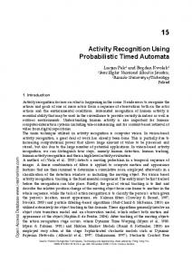
We interviewed the participants and collected ground truth (5 mins) of the predominant locomotion/posture change activities and trained our classifiers. We had 6 activities in the ground truth study – {‘stand’, ‘walk slowly’, ‘sit relaxed’, ‘sit’, ‘normalWalk’, ‘stairs’}. Thereafter, we ran the A3R algorithm on the continuous data traces (using a frame size of 5 secs) and extracted a sequence of activity inferences and A3R state transitions. Fig. 5 shows the total number of activity instances (for all 6 activities), for the complete N95 traces of 6 users. Even though the classifier output may be erroneous (we cannot possibly have ground truth for the entire 6-8 weeks), we believe that the results are reasonably accurate, given the ≥ 90% accuracy observed during training & cross validation of the 5 mins ground truth data. Fig. 6 shows the histogram of the durations for which each activity instance lasted. We observe that the classifier indicates that the vast majority of individual activity instances lasts for several minutes (1 min = 12 activity frames in the plot), with most instances lasting at least 1-2 mins. This observation also justifies the use of Wf rame = 10 in our sliding window computation. We also observe that siting activities (‘sit’ and ‘sitRelax’) typically have longer durations than ‘stand’ & ‘slowWalk’ activities, which, in turn, last longer than more active motions (e.g., ‘normalWalk’ and ‘stairs’). Table 4 reports the emulated energy consumption, based on the N95 data traces, if the user activities had been monitored by the Galaxy S2 phone. The figures are obtained by
4
x 10
5
sitRelax
normalWalk
slowWalk
stand
stairs
14 12 10 8 6 4 2 0
user1
user2
user3
user4
user5
user6
58
10
sit sitRelax normalWalk slowWalk stand stairs
4
10
3
10
2
10
1
10
0
user2
user3
user4
user5
54 52 50 48
5
10
15
20
25
duration of continuous activities (frame)
30
5
10
15
20
Figure 6: Distribution of continuous activi-
Figure 7: Impact of window size on
for Nokia Users in our observation period
ty lengths detected for N95 Users
energy savings in A3R
using the sequence of A3R state transitions observed and multiplying each such activity duration by the corresponding energy power consumption data (from Table 3) for the corresponding hSF, CF i state. The table shows the battery consumption for 5 different cases: • Full100, Full50, Full16, Full5: Four non-adaptive scenarios, where the sampling frequency is always kept fixed at either {100, 50, 16, 5} Hz and classification always uses both time and frequency domain features being computed continuously; • A3R: Dynamically adjust the smart hSF, CF i choice in Table 3 according to the state. We compute the energy save compared to the full power mode F ull100, ull100)−energy(A3R) i.e., energy(F × 100%. energy(F ull100) Table 4: Cross-user Study of Energy Savings obtained by running Activity Trace through different modes of Continuous Recognition Engine (A3R is using Wf rame =10 and ∆conf =0.6) Time (hour) 102.6 207.4 216.7 139 143.9 139.8
Full100 (J) 23675 47857.6 50003.5 32074.3 33204.9 32258.9
Full50 (J) 16251.8 32852.2 34325.3 22017.6 22793.8 22144.3
Full16 (J) 12301.7 24867.3 25982.3 16666.1 17253.6 16762
Full5 (J) 7777.1 15720.9 16425.9 10536.2 10907.6 10596.8
A3R Energy (J) Save (%) 12052.1 49.09 23817.4 50.23 22206.2 55.59 15192.4 52.63 16812.1 49.37 14715.4 54.38
We find that A3R’s energy consumption is approximately 50% less than a continuous sensing engine running at full power (100 Hz). Further, the figure demonstrates that A3R’s energy consumption is lower than even sampling constantly @16Hz, with the advantage of improved accuracy, especially for the more-vigorous activities. Parameters Analysis: Fig. 7 studies the effect of window size (Wf rame ) used in A3R w.r.t. energy loss. Initially, a higher value of Wf rame (greater smoothing) implies a lower likelihood that erroneous readings or random transient movements will cause a transition to the ‘unknown state’. However, as Wf rame grows beyond 10 frames (i.e., 50 seconds), a single window will have an increasing mix of 2 (or more) different consecutive activities, causing the
25
Window Size (frames)
Figure 5: Distribution of activities detected
User ID 1 2 3 4 5 6
user6
56
46
0
10
user1
Energy Saved by A3R (%)
sit
count of continuous activities
count of activities
16
classification confidence to be lower, thereby causing more frequent transititions to the power-hungry ‘unknown’ state. Fig. 8 shows the energy savings as the desired confidence level (∆conf ) is varied. Naturally, a lower confidence threshold allows A3R to remain in a known activity state longer, at reduced sampling rates, but can compromise the prediction accuracy. A higher confidence threshold on the other hand makes A3R jump to the more energy-expensive unknown state more often. In all cases, the energy savings (over the Full100 non-adaptive approach) is seen to vary between 45-55% across users.
5.2
In-Situ Study for Android Users
We also experimented with an Android-based implementation of A3R, used by 2 users each for a span of 6 days. The study was divided into 3 scenarios and the study was repeated for 2 days per scenario. • Non-adaptive: The non-adaptive scenario, where the sampling frequency is always kept fixed at {50} Hz and classification always uses both time and frequency domain features being computed continuously • A3R: The adaptive scenario, where A3R is used to dynamically adjust the hSF, CF i parameters. • No activity recog.: The baseline, where there is no activity prediction application running on the phone. We recorded the battery level using android’s BatteryManager API, as the users went about performing their daily activities (e.g., call, SMS, browsing). While the phone battery was charged overnight each day, ensuring an identical starting condition, the daily browsing and digital consumption patterns would vary randomly each day. However, the days selected were all ‘normal’ weekdays, which were likely to exhibit similar mobile usage behavior. User1 started his day around 7:30AM, while user 2 starts around 8:00 AM. Fig. 9 reflects the battery drainage time series for each user (averaged over the 2 days per scenario) for the 3 scenarios. We can see ocassional sharp drops in battery levels, due to sporadic high load spikes (e.g., a long phone
50 45
user1 user2 user3 user4 user5 user6
40 35 30 0.3
0.4
0.5
0.6
0.7
0.8
0.9
90 80 70 60 50 40
User1 A3R Non-‐adapBve No acBvity recog
30
Confidence Threshold
Ba/ery Remaining (% age)
55
100
100 90 80 70 60 50
User 2 A3R Non-‐adapBve No acBvity recog.
40 30 7: 56 8: 26 8: 55 9: 26 9: 57 10 :2 5 10 :5 0 11 :1 9 12 :0 5 12 :3 6 13 :0 7 13 :3 7 15 :3 4
Ba/ery Remaining (% age)
60
7: 37 8: 20 8: 59 9: 3 10 7 :1 10 5 :5 11 4 :3 12 2 :1 12 0 :4 13 9 :2 14 6 :0 14 6 :4 15 4 :2 16 2 :0 16 1 :4 17 0 :1 8
Energy Saved by A3R (%)
65
Time
Time
Figure 8: Impact of confidence threshold on
Figure 9: Power consumption of different activity recognition modes in daily lifestyle
energy savings in A3R
settings (evaluating the embedded A3R for two Android users)
call, or a sudden period of video browsing); accordingly, it is possible that, ocassionally, the phone battery level was lower in the absence of activity recognition than when A3R was used (see 8:30-9:30am in User2’s plot). Nevertheless, we can observe that at the end of a regular day, the A3R algorithm clearly saves 20-25% of battery power as opposed to the non-adaptive recognition scenario. This lower amount of overhead reduction (compared to the N95 study) is likely due to that this data includes the subject(s) engaging in other random (beyond the 6 labeled) activities, causing A3R to transition to the higher energy consuming, ‘unknown’ state more often.
6
Conclusion
This paper presented an empirical investigation of energy consumption characteristics of real-time activity recognition applications, executing continuously on mobile phones. We report how Sampling Frequency (SF) and Classification Features (CF) alter the energy consumed in recognition. After demonstrating that different activities require different combinations of hSF, CF i to achieve the desired accuracy levels, we devised the “A3R” algorithm, and evaluated it using two types of naturalistic data (1) 6 Nokia N95 users over longer spans of times (6-8 weeks) and (2) insitu study of two Android users. Our investigation indicates that such an activity-adaptive model holds potential for significantly reducing the energy overheads of accelerometerbased continuous mobile sensing.
References [1] L. Bao and S. Intille. Activity Recognition from UserAnnotated Acceleration Data. In Pervasive, pages 1–17, 2004. [2] D. Chu et. al. Balancing Energy, Latency and Accuracy for Mobile Sensor Data Classification. In ACM Sensys’11, pages 54–67, 2011. [3] F. Foerster, M. Smeja, and J. Fahrenberg. Detection of posture and motion by accelerometry: a validation study in ambulatory monitoring. Computers in Human Behavior, 15(5):571 – 583, 1999.
[4] T. Gu, Z. Wu, X. Tao, H. K. Pung, and J. Lu. epSICAR: An Emerging Patterns based Approach to Sequential, Interleaved and Concurrent Activity Recognition. In PerCom, pages 1–9, 2009. [5] H. Junker, P. Lukowicz, and G. Troster. Sampling Frequency, Signal Resolution and the Accuracy ofWearable Context Recognition Systems. In ISWC, pages 176–177, 2004. [6] A. Krause et. al. Trading off Prediction Accuracy and Power Consumption for Context-AwareWearable Computing. In ISWC, pages 20–26, 2005. [7] H. Lu, A. Brush, B. Priyantha, A. Karlson, and J. Liu. SpeakerSense: Energy Efficient Unobtrusive Speaker Identification on Mobile Phones. In Pervasive, pages 188–205, 2011. [8] H. Lu, J. Yang, J. Liu, N. Lane, T. Choudhury, and A. Campbell. The Jigsaw Continuous Sensing Engine for Mobile Phone Applications. In Sensys, pages 71–84, 2010. [9] E. Miluzzo, N. Lane, K. Fodor, R. Peterson, H. Lu, M. Musolesi, S. Eisenman, X. Zheng, and A. Campbell. Sensing Meets Mobile Social Networks: the Design, Implementation and Evaluation of the Cenceme Application. In Sensys, pages 337–350, 2008. [10] B. Priyantha, D. Lymberopoulos, and J. Liu. Littlerock: Enabling energy-efficient continuous sensing on mobile phones. IEEE Pervasive Computing, 10(2):12–15, 2011. [11] K. Rachuri, C. Mascolo, M. Musolesi, and P. Rentfrow. SociableSense: Exploring the Trade-offs of Adaptive Sampling and Computation Offloading for Social Sensing. In MobiCom, pages 73–84, 2011. [12] G. Raffa, J. Lee, L. Nachman, and J. Song. Don’t slow me down: Bringing Energy Efficiency to Continuous Gesture Recognition. In ISWC, pages 1–8, oct. 2010. [13] N. Ravi, N. Dandekar, P. Mysore, and M. L. Littman. Activity Recognition from Accelerometer Data. In AAAI, pages 1541–1546, 2005. [14] Y. Wang, J. Lin, M. Annavaram, Q. Jacobson, J. I. Hong, B. Krishnamachari, and N. M. Sadeh. A Framework of Energy Efficient Mobile Sensing for Automatic User State Recognition. In MobiSys, pages 179–192, 2009. [15] Z. Yan, D. Chakraborty, A. Misra, H. Y. Jeung, and K. Aberer. SAMMPLE: Detecting Semantic Indoor Activities in Practical Settings using Locomotive Signatures. In ISWC, 2012. [16] J. Yang, H. Lu, Z. Liu, and P. Boda. Physical Activity Recognition with Mobile Phones: Challenges, Methods, and Applications. In Multimedia Interaction and Intelligent User Interfaces, pages 185–213, 2010.