This full text paper was peer reviewed at the direction of IEEE Communications Society subject matter experts for publication in the ICC 2008 proceedings.
Energy-Efficient Data Dissemination Protocol for Detouring Routing Holes in Wireless Sensor Networks Ye Tian, Fucai Yu, Younghwan Choi, Soochang Park, Euisin Lee, Minsook Jin, and Sang-Ha Kim* Dept. of Computer Engineering Chungnam National University, 220 Gung-dong, Yuseong-gu, Daejeon, 305-764, Republic of Korea {tianye, yufc, yhchoi, winter, eslee, badamul}@cclab.cnu.ac.kr and
[email protected] Abstract—Void areas (holes) as an inevitable phenomenon exist in geographic routing of wireless sensor networks, because the unpredictable and harsh nature application environment or uneven energy consumption. Most of the existing schemes for the issue tend to construct a static detour path to bypass a hole. The static detour path may lead to uneven energy consumption of the nodes on the perimeter of the hole; thus it may enlarge the hole. At the same time, traffic would concentrate on the peripheral node of the hole; thus the nodes on the perimeter of the hole tend to be depleted quickly. In previous work, we have proposed a hole geometric model to reduce the energy consumption and packet collisions of the nodes on the hole boundary. This scheme, however, still has the static detour path problem. Therefore, we extend the previous work by constructing a dynamic detour path hole geometric model for wireless sensor networks in this paper. The location of hole detour anchor is dynamically shifted according to Gaussian function, just generating dynamic hole detour paths. Keywords-sensor networks, geographic routing, energy efficient, hole problem
I.
INTRODUCTION
A wireless sensor network (WSN) consists of a large number of unattended sensor nodes which self-organize themselves into a communication network. These sensor nodes collaborate among themselves to collect, process, analyze and disseminate data. Limitation of sensor nodes in terms of memory, energy, and computation capacities give rise to many research issues in wireless sensor networks. Among these limitations, energy consumption of sensors is a major issue when designing routing protocols in wireless sensor networks. Geographic routing has been considered as an attractive approach since it exploits pure location information instead of global topology information to route data packets, this location based scheme makes it a more efficient, simple and scalable routing protocol in wireless sensor networks [1-5]. This mechanism can minimize the hops from the source to the destination. Holes, it also called local minimum phenomenon [5], as
an inevitable phenomenon exist in geographic routing. Among existing routing protocol in the literature [7], most existing geographic routing protocols adopt static and peripheral mode bypass holes. GPSR [1] handles hole problem by deriving a planar graph out of the original network graph. In GPSR, traffic would concentrate on the peripheral node of the hole. Compass Routing II algorithm [8], also guarantees that the data packets can reach destination even when holes existing in greedy forwarding. They proposed routing protocol using the least deviation angle from the line joining the node to the destination when trying to transmit a packet to the next hop. [3] proposed the FACE-1 and FACE-2 routing algorithms to guarantee packet delivery in mobile ad hoc network (MANET). The adopted solution is also based on getting a connected planar subgraph by using Gabriel Graph and then traversing the edges of the graph using right-hand rule. In contrast to GPSR, all routing is done through the perimeter of the GG formed at each node. FACE-2 modifies FACE-1 in that the perimeter traversal follows the next edge whenever that edge crosses the line from the source to destination. To sum up the above protocols, the routing hole algorithms are always addressed by using the static and perimeter mode routing. Before the nodes on the perimeter die, packets are always delivered by the peripheral node of the hole. Consequently, the derived planar graph is much sparser than the original one, and the traffic concentrates on the perimeter of the planar graph. Thus, the nodes on the perimeter tend to be depleted quickly, at the same time, it may incur data collisions. In previous work [9], we have proposed a hole geometric model to reduce the energy consumption and data collisions on the perimeter of the planar graph. This scheme, however, still using the static detour path routing holes which means the nodes along this path their energy deplete quickly than general nodes. Therefore we extend the previous work by constructing a dynamic detour path hole geometric model for balance energy consumption. The location of hole detour anchor point is dynamically shifted according to Gaussian function, just generating dynamic hole detour paths.
*Sang-Ha Kim is corresponding author with the Department of Computer Engineering, Chungnam National University (email:
[email protected]).
978-1-4244-2075-9/08/$25.00 ©2008 IEEE
This full text paper was peer reviewed at the direction of IEEE Communications Society subject matter experts for publication in the ICC 2008 proceedings.
the longest distance among the distances between any two nodes in {B0, B1…Bn}. Then on each side of B p Bq a node that the vertical distance from it to
B p Bq is
longer than other hole
boundary nodes on corresponding side of
B p Bq
e.g., Bj and Bk,
is selected by node B0. Then through Bp, Bj, Bq and Bk, node B0 can obtain a rectangle, and the bisectors of four right angles of the rectangle intersect at point F1 and F2 with the coordinates (x1,y1) and (x2,y2) as shown in Fig.1-3. Then node B0 selects Bm from {B0, B1…Bn} so that the sum distances of Bm F1 and Bm F2 is the longest than that of other nodes in {B0, B1…Bn} as shown in Fig.1-4. Assume that Bm F1 + Bm F2 = 2a, then according ellipse definition function, B0 defines an ellipse as: (x − x1 )2 + (y − y1 )2 + (x − x2 )2 + (y − y 2 ) 2 = 2a , Figure 1. Hole geometric modeling processes
The rest of this paper is organized as follows: We briefly discuss related work in Section II. We explain our protocol in Section III and detailed analysis of our protocol is given in section IV. Section V is the simulations and comparisons, section VI concludes the paper. II. RELATED WORK To make every detail clearly, we first briefly introduce the previous work [9]. Fig.1 shows hole geometric modeling processes. As shown in Fig. 1-1 by real line, when a data packet is sent by geographic forwarding mechanism reaches a node (suppose node U) on the ellipse (not hole), node U redirects the data packet along the tangent direction of the ellipse with a distance L to another location. When the node (suppose node V) which is geometrically closest to that location receives the data packet, it redirects the data packet to original destination by geographic forwarding mechanism. The rest of this section explains how to construct the ellipse to cover the hole and define a proper length L. The rest parts of Fig.1 shows hole geometric modeling processes. A node can detect whether it is locating on the boundary of a hole by the mechanism proposed in [5]. The node which firstly detects a hole sends out a Hole Boundary Detection (HBD) packet along the boundary of the hole by the well-known right hand rule [6]. The mission of HBD packet is to trace the location information of all nodes on the boundary of the hole. We suppose that nodes B0, B1…Bn, with the coordinates (x0, y0), (x1, y1)… (xn, yn) are on the boundary of a hole. As shown in Fig.1-2, node B0 firstly detects that it is locating on the boundary of the hole, it initiates a HBD packet marked with its ID and forwards the HBD packet to hole boundary node B1 by right hand rule. Node B1 inserts its location information into the received HBD packet and forwards it to node B2 by right hand rule too. This process repeats until the HBD packet has traveled around the hole and eventually been received by the initiator node B0. Node B0 gets the location information of all boundary nodes of the hole from receiving HBD. Then node B0 selects two nodes Bp and Bq from {B0, B1…Bn} so that the distance between Bp and Bq is
(1)
Where a is the semimajor axis of the ellipse. Assume the distance between F1 and F2 in Fig.1-3 is 2c, and then according to ellipse property, we can get the semiminor axis of the ellipse b as: b = a2 − c2 ,
(2)
So far, we get the ellipse which can cover the hole exactly. Then node B0 initiates an Ellipse Distribution (ED) packet which includes all information about the ellipse, and geocasts the ED packet to all nodes inside the ellipse. Then all nodes inside the ellipse are aware of the ellipse as shown in Fig.1-4. Now, we introduce how to calculate the anchor location. In previous algorithm that the anchor locates on the tangent line through tangent point U to the ellipse. As shown in Fig.1-1by real line, V is anchor point of U for the packet destined to destination D. Line UV is tangent to the ellipse through tangent point U. According to plan geometric theory, node U can get the location of V if it knows the length L. Node U calculates L by following formula:
L = a ⋅ b( 1 + α) − d , 0 ≤ α ≤ 1 ,
(3)
Where a is the semimajor axis of the ellipse, b is the semiminor axis of the ellipse, d is the vertical distance from the centre of the ellipse to line UD and α is a balance parameter set by system. Since node U knows the location of itself and all information about the ellipse (got from ED message). The location of destination D can be gotten from the received data packet. Then it is definitely that node U can calculate out d (the calculation method is not covered in this paper). Up to now, L becomes a known quantity, thus node U can get the location information of V. III.
ENERGY-EFFICIENT DATA DISSEMINATION PROTOCOL FOR DETOURING ROUTING HOLES
A. Preparation Work So far, we get the location of anchor point which is defined in static condition. It means the path between tangent point and destination does not change unless the network topology changes. As a result, the nodes on this path drain their energy
This full text paper was peer reviewed at the direction of IEEE Communications Society subject matter experts for publication in the ICC 2008 proceedings.
static anchor point. It may occur that no node at the location (a + u, b + v). In this situation, we select the geographically closest one as the dynamical anchor point.
Figure 2. Dynamically data delivery scenarios of hole geometric modeling
much faster than general nodes. As mentioned in the introduction, we try to construct a dynamic detour path hole geometric model for balance energy consumption. Now, we describe the Energy-efficient Data Dissemination Protocol for Detouring Routing Holes in Wireless Sensor Networks. We balance energy consumption through the dynamical anchor point. Same to previous work, the dynamical anchor point is still determined by the node which is on the boundary of the hole. In addition, for optimizing entire routing process, we modify the set of all possible values of the balance parameter α. As step 1, the tangent node calculates L will follow (4):
L = a ⋅ b( 1 + α) − d 0.2≤ α ≤1.2,
(4)
The length L between the tangent point node and the anchor point node which is defined in (4) is longer than length L which is defined in (3). We get the anchor point through (4), and we suppose the coordinate of the anchor point is (a, b). Our promoted protocol has two main steps about how to get the dynamical anchor point. Step1, tangent point node gets the basic location information of anchor point using (4). Step2, base on the 2-dimensional Gaussian function anchor point dynamically shifted. The 2-dimensional Gaussian function is following:
f(u,v)
1 = 2 πσ
2
e
−
(u
2
+v2 )
2σ
2
(5)
This formula produces a surface whose contours are concentric circles with a Gaussian distribution from the center point. In our promoted protocol, the coordinate of the anchor point node (a, b) is substituted by the dynamically shifted coordinate (a + u, b + v), u, v is the location increment variable. Anchor point which is gotten form (4) only as the centre point of concentric circles, we call it basic anchor point. And then, the tangent point node of the hole will send the packet to the dynamically changed anchor point instead of the
B. Data Delivery Under Hole Geometric Modeling Up to now, all of the preparation work has been done. The following section, we depict the data transmission process from source to destination. As shown in Fig.2 where only hole geometric modeling ellipse and data delivery paths are represented. In Fig.2, the real line indicates only one of the optional routing paths according to our algorithm. Circle indicates entire possible area where anchor point may locate in. Data transmission process follows the one of the existing geographic routing protocol. Source node S initiates data packets and transmits them to destination node D and each data packet header contains an anchor location field and a flag field which indicating the data packet transmission in anchor transmission mode or in destination transmission mode. At the initial phase, all data packets are set to destination transmission mode and their anchor location field is set to void state by source. Source also adds the geographic location information of the destination in data packets. Destination location field is only set by source, and left unchanged as the packet is forwarded through the network. In Fig.2-1, source node S transmits a data packet to destination D along the line SD by one of the existing geographic routing protocol. Nodes on the ellipse are distinguished with the others by ED packet information which is existent in nodes on the ellipse. When data packet reaches the boundary of the ellipse, it sets the data packet to anchor mode, and adds the anchor location information to the data packet which is calculated by (4) and (5), and then forwards the data packet to the node which is geographically closest to the anchor location. When the node closest to the anchor location receives the data packet, it resets the data packet to destination transmission mode and resets anchor location field to void state, then transmits the data packet to destination directly. IV.
ANALYSIS
Geographic protocols, that take advantage of the location information of nodes, are very valuable for sensor networks. The state required to be maintained is minimum and their overhead is low, in addition to their fast response to dynamics. Its routing path fleetly adapts to variational location of mobile source or destination, source node is not required to be aware of network global information, thus it competently supports source mobility. Our mechanism also possesses these advantages. Only the sensor nodes inside the ellipse are aware of the hole, all other nodes are blind to the hole, even the source node. In some sense, we can regard the ellipse as a shield. In our algorithm, different source nodes may have same tangent point nodes, but their anchor point nodes must different based on our formula of anchor point. And the routing path changing with time can totally avoid uneven energy consumption. In (4) the L and d is a constant value, and we extend the set of all possible values of the balance parameter α, so that reduce the
This full text paper was peer reviewed at the direction of IEEE Communications Society subject matter experts for publication in the ICC 2008 proceedings.
probability of the data packet reencounter the circle. For balance energy consumption, we adopt 2-dimensional Gaussian function. In practice, when computing a discrete approximation of the Gaussian function, points outside of approximately 3σ are small enough to be considered effectively zero. Thus, anchor point outside of that range can be ignored. In our algorithm, we set the standard deviation σ of two-dimensional Gaussian distribution equal to sensor node transmission range. From (4) we can see the balance parameter α affects the length of L, a short L may cause the data packet from anchor node to destination node encounter the ellipse again. We cannot prevent such things from occurring in our protocol because the unpredictable and harsh nature application environment or uneven energy consumption. We evaluate the affection of α by simulation in next section. Another condition is that the destination node D locates closely to the ellipse, as shown in Fig.2-2. In this case, the data packet is redirected to another anchor point from node U1. In Fig.2-3, the anchor location of node U locates inside another ellipse. In this case, when the node on the ellipse receives the data packet from U, it also resets the packet in destination mode and set anchor location in void state, then forwards the packet to original destination by geographic forwarding mechanism. Fig.2-4 shows that our algorithm is available in the condition of several holes existing between source and destination. If the data packet from the first agent location to destination encounters another ellipse, the data packet is redirected to another agent location again. This process repeats until the data packet reaches original destination. V. PERFORMANCE E VALUATIONS In this section, we evaluate the performance of our algorithm by simulation. First we depict our performance metrics and simulation environment. Then we evaluate the system performance with given environment and parameters. Finally, we show the comparisons between our scheme, GPSR, SPEED [10] and our previous work. A. Simulation Environments and Metrics We implemented our algorithm in Network Simulator Qualnet 3.8 and selected IEEE 802.11 as MAC protocol. The transmission range of sensor nodes is 150 m. The size of the sensor network is set to 2000*2000 m2 where 10,000 nodes are randomly distributed. The average distance between nodes is 20 m. we manually set three holes in the network with the coverage about 400*200 m2, 300*200 m2 and 200*200 m2. 5 sources and 5 destinations are moving with a random speed of 0m/s~2m/s. And the destination location is known by the corresponding source. Each simulation lasted for 1000s. We employ three metrics to evaluate the performance of our algorithm. The packet delivery ratio is the ratio of the number of successfully delivered data packets to the number of data packets generated by the source. This metric reflects the data delivery efficiency. Energy consumption is the total energy consumption of the nodes around the hole. The metric reflects the trend of the change of the network topology. Network lifetime extension ratio is the ratio of the network
lifetime prolonging. This metric reflects our protocol effect on reduce energy consumption of sensor networks. B. Simulation Results 1) Effect of α in Hole Geometric Modeling: Fig.3 shows the packet delivery ratio affected by α. From formula (4) we can see α affects the length of L, thus affects anchor location. In Fig.3, the packet delivery ratio increases while increasing α from 0.2 to 0.4. In our simulation, five sources send data packets to five destinations simultaneously. When α > 0.4, the packet delivery ratio decreased. The reason is that, with increasing α, the length of the data transmission path is increased. 2) Performance Comparisons with Other Protocols: We compare the packet delivery ratio, energy consumption with GPSR, SPEED and compare the network lifetime with original work through different number of communication sessions in this section. Fig.4 shows the packet delivery ratio with different number of communication sessions. When there is only one communication session (one source and one destination), four protocols almost achieve the same packet delivery ratio. This is because almost no collision occurs during simulation time. Only a few data packets may be lost due to source and destination mobility. With the number of communication session increasing, multiple communication sessions may need to bypass a hole simultaneously. GPSR and SPEED forward data packets along holes boundaries by the right hand rule. So the probability that data collisions occur in the nodes around the hole is increased with an increasing number of communication sessions. However both our original work and promoted algorithm, the data packets are redirected to anchor location once they encounter a hole, the anchor location is different with different sources or destinations. Thus the probability of data collisions does not markedly increase with the increasing number of communication sessions. So packet delivery ratio of our algorithm does not markedly decrease with an increasing number of communication sessions. Fig.5 shows the total energy consumption of nodes on boundary of holes. GPSR and SPEED utilize right hand rule to route data packet to destination when the data packet encounters a hole, in other words, as long as a hole locates between source and destination, the data packet must be sent along the boundary of the hole. Thus the energy consumption of the nodes on the boundary of holes is quite high in SPEED and GPSR. Our protocol, firstly, the data packet is redirected to anchor location when the data packet encounters an ellipse. By this way to prevent data packet go along the boundary of holes. Thus reduce energy consumption of the nodes on the boundary of holes and prevent holes diffusion. Secondly, the anchor location intimately related to source and destination location. It means the data delivery path near a hole is different with variational source or destination location. Fig.6 shows the Network lifetime extension ratio between original algorithm and promoted protocol. In this figure, we set all communication sessions of original work equal to 100%,we only show the relative ratio of network lifetime
This full text paper was peer reviewed at the direction of IEEE Communications Society subject matter experts for publication in the ICC 2008 proceedings.
Figure 3. Packet delivery ratio effected by α
Figure 4. Packet delivery ratio with different number of communication sessions
Figure 5. Energy consumption with different number of communication sessions
Figure 6. Network lifetime comparison between original work and promoted protocol
extension. Our promoted protocol through dynamically shifted anchor point balance energy consumption of nodes around hole. Simulation result shows, our promoted algorithm is effective in prolonging the lifetime of the sensor networks. It can extend the lifetime of network up to 12% to 23%. VI. CONCLUSIONS In this paper we proposed energy-efficient data dissemination protocol for detouring routing holes mechanism which is not only models a hole by an ellipse to solve holes problem but also construct a dynamical routing path to balance energy consumption in sensor network. The node on the boundary of ellipse redirects the received data packets to anchor location, therefore bypassing hole area. Our algorithm has three prominent advantages: (a) it prevents data packets from entering the stuck area of a hole, thus reducing route rediscovery overhead; (b) it reduces energy consumptions and data collisions of the node on the boundary of hole.(c) it balances energy consumption of the entire hole existing area. REFERENCES [1]
[2]
B. Karp, H. T. Kung. GPSR: Greedy perimeter stateless routing for wireless networks. In: Proc. ACM/IEEE International Conf. on Mobile Computing and Networking. Boston, MA, Aug. 2000, pp.243-254. F. Kuhn, R. Wattenhofer, Y. Zhang, and A. Zollinger, “Geometric adhoc routing: of theory and practice,” in Proc. ACM Symposium on the
Principles of Distributed Computing (PODC), Boston, MA, Jul. 2003, pp. 243–254. [3] P. Bose, P. Morin, I. Stojmenovic, and J. Urrutia, “Routing with guaranteed delivery in ad hoc wireless networks,” in Proc. of the 3rd International Workshop on Discrete Algorithms and Methods for Mobile Computing and Communications, pp. 48–55, 1999. [4] Y. B. Ko and N. H. Vaidya, “Location-aided routing (LAR) in mobile adhoc networks,” in Proc. ACM/IEEE International Conference on Mobile Computing and Networking (MobiCom), Dallas, TX, Oct. 1998, pp. 66–75. [5] Q. Fang, J. Gao, und L. J. Guibas, “Locating and bypassing routing holes in sensor networks”. In Proc. of INFOCOM 2004, vol.4, March 2004 pp.2458-2468. [6] J.A. Bondy and U.S.R. Murty, Graph Theory with Applications (Elsevier North-Holland, 1976). [7] N. Ahmed, S. S. Kanhere and S. Jha, "The Holes Problem in Wireless. Sensor Networks: A Survey," ACM SIGMOBILE Mobile Computing. and Communications Review, vol. 9, pp. 4 - 18, 2005. [8] E. Kranakis, H. Singh, and J. Urrutia. Compass routing on geometric networks. In Proceedings of the 11th Canadian Conference on Computational Geometry (CCCG'99), 1999. [9] F.C. Yu, E. Lee, Y.Choi, S. Park, D. Lee, Y. Tian, and S. Kim, “A Modeling for Hole Problem in Wireless Sensor Networks,” In Proc. of the IWCMC'07, August 12-16, 2007, Honolulu, Hawaii, USA. [10] T. He, J.A. Stankovic, C. Lu and T.F. Abdelzaher, “A Spatiotemporal Communication Protocol for Wireless Sensor Networks”, IEEE Transactions on Parallel and Distributed Systems, VOL. 16, NO. 10, October 2005, pp.995-1006.