Energy-Efficient Link-Layer Jamming Attacks against Wireless Sensor

Energy-Efficient Link-Layer Jamming Attacks against Wireless Sensor Network MAC Protocols Yee Wei Law

Lodewijk van Hoesel

Jeroen Doumen

Pieter Hartel

Paul Havinga

Faculty of Electrical Engineering, Mathematics and Computer Science University of Twente, P.O. Box 217, 7500AE Enschede, The Netherlands {yee.wei.law, lodewijk.vanhoesel, jeroen.doumen, pieter.hartel, paul.havinga}@utwente.nl

ABSTRACT A typical wireless sensor node has little protection against radio jamming. The situation becomes worse if energyefficient jamming can be achieved by exploiting knowledge of the data link layer. Encrypting the packets may help prevent the jammer from taking actions based on the content of the packets, but the temporal arrangement of the packets induced by the nature of the protocol might unravel patterns that the jammer can take advantage of even when the packets are encrypted. By looking at the packet interarrival times in three representative MAC protocols, S-MAC, LMAC and B-MAC, we derive several jamming attacks that allow the jammer to jam S-MAC, LMAC and B-MAC energy-efficiently. The jamming attacks are based on realistic assumptions. The algorithms are described in detail and simulated. The effectiveness and efficiency of the attacks are examined. Careful analysis of other protocols belonging to the respective categories of S-MAC, LMAC and B-MAC reveal that those protocols are, to some extent, also susceptible to our attacks. The result of this investigation provides new insights into the security considerations of MAC protocols. Categories and Subject Descriptors: C.2.0 ComputerCommunication Networks: General – Security and Protection General Terms: Security, algorithms. Keywords: MAC protocols, security, denial-of-service attacks, jamming, clustering.

1.

INTRODUCTION

Jamming-style DoS attacks on the physical and data link layer of WSNs have in these few years attracted some attention [20, 40, 44, 45]. In particular, Xu et al. [44] propose 4 generic jammer models, namely (1) the constant jammer, (2) the deceptive jammer, (3) the random jammer and (4) the reactive jammer. A constant jammer emits a constant noise; a deceptive jammer either fabricates or replays valid signals

Permission to make digital or hard copies of all or part of this work for personal or classroom use is granted without fee provided that copies are not made or distributed for profit or commercial advantage and that copies bear this notice and the full citation on the first page. To copy otherwise, to republish, to post on servers or to redistribute to lists, requires prior specific permission and/or a fee. SANS’05, November 7, 2005, Alexandria, Virginia, USA. Copyright 2005 ACM 1-59593-227-5/05/0011 ...$5.00.

on the channel incessantly; a random jammer sleeps for a random time and jams for a random time; and lastly, a reactive jammer listens for activity on the channel, and in case of activity, immediately sends out a random signal to collide with the existing signal on the channel. According to Xu et al. [44], the constant jammers, deceptive jammers and reactive jammers are effective jammers in that they can cause the packet delivery ratio to fall to zero or almost zero, if they are placed within a suitable distance from the the victims. However these jammers are also energy-inefficient, meaning they would exhaust their energy sooner than their victims would if given comparable energy budgets. Although random jammers save energy by sleeping, they are less effective. Our contribution is to develop jamming attacks that (1) work on encrypted packets, (2) are as effective as constant /deceptive/reactive jamming, and (3) at the same time more energy-efficient than random jamming or reactive jamming. We implement such jamming attacks by exploiting the semantics of the data link layer and show the results quantitatively. The fact that our attacks are applicable to three representative MAC protocols suggests the same attacks are applicable to a wide range of other protocols belonging to the same categories as these protocols’. Our analysis of the attacks provides new insights into the timing considerations of MAC protocols with regards to security, and provides hints on which category of protocols provides the best protection against our attacks so far, in the absence of effective countermeasures. The motivation of this work stems from the concern that if an attacker can program and deploy a general-purpose link-layer jamming network that is able to jam any WSN effectively and energy-efficiently, and if a high entry barrier is not maintained for such a low cost attack, a WSN can never in any practical sense be secure. A counterargument might be that energy efficiency is no concern to powerful attackers, but even powerful jammers come with a finite energy supply and they would advertise their presence and location if they simply blast away with an exorbitant amount of radio waves – this is something a sensible attacker would avoid. The paper is organized as follows. We start by stating the assumptions on which our attacks are based in Section 2. We then describe the attack algorithms in Section 3. Section 4 describes how the protocols and the corresponding attacks are simulated, and how the results are evaluated. The results are given in Section 6. Implications of our work to other protocols are discussed in Section 7. Section 8 explores some potential countermeasures. Related work is discussed in Section 9. Finally Section 10 concludes.

2.

ASSUMPTIONS

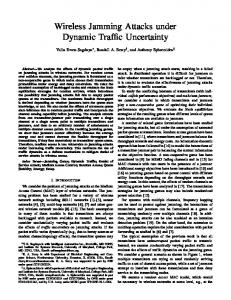
We assume an attacker has two goals: the primary goal is to disrupt the network by preventing messages from arriving at the sink node, and the secondary goal is to increase the energy wastage of the sensors. A sink node is a node that requests for, and hence sinks, information. Our attacks depend on three assumptions: (1) the jammer motes know the preamble used by the victim nodes, (2) the jammer motes can measure the length of a packet, and (3) the jammer motes know what MAC protocol that victim notes are running. A preamble is a bit sequence, usually consisting of alternating 1’s and 0’s, for training the receiver, and its length depends on the data coding scheme used [34]. Requirement (1) and (2) should be easy to satisfy in practice. Requirement (3) is more demanding but not impractical to satisfy – as our future work, a strategy will be devised to map observed traffic to specific classes of protocols. Note that the jammer motes do not need to know the content of the packets, so our attacks work even if the packets are encrypted. Adding to the significance of our attacks is that the attacker does not need to capture and compromise any existing sensor nodes. Jammer motes

Interceptor informs motes of estimated frequencies

Sensor nodes

Figure 1: Distributed jamming. We now describe a concrete set of circumstances under which our attack scenario is applicable. • When there are no fixed sink nodes to attack, e.g. in directed diffusion [12] where ID-less interests propagate through the network, there is no way for a node to tell where the real sinks are, • or when it is infeasible for the attacker to deploy its nodes strategically, except perhaps to air-drop them on top of the target network, • or when the attacker can only estimate where and not how the target network is or would be deployed, • or when the target network is protected with a linklayer authentication (and optionally encryption) scheme like TinySec [15], the attacker would find it appealing to distribute its jammer motes among the target WSN and apply our jamming attacks. We are in fact not alone in suggesting this attack scenario [27]. One note of caution though, is that if the target network employs frequency-hopping spread spectrum [1], the attacker would find it necessary to deploy an interceptor to discover the hopping frequencies first before its network of jammer motes can start jamming (Figure 1). Naturally, our attacks are affected by the choice of values assigned to the protocol parameters. Throughout the paper, we pick values for the protocol parameters that are either

as realistic or as faithful to what the creators of the protocols recommend as possible, in the absence of a universal consensus and a scientifically rigorous way of deriving these values.

3.

MAC PROTOCOLS FOR WSNS

Before we describe our attacks, a brief overview of MAC protocols for WSNs is in order. Despite the number of protocols proposed so far, there is still no clear indication of the mechanisms the proposals are converging to [19]. However, since different applications require optimizing different parameters, there will most likely not be a single solution that fits all types of applications. According to Langendoen et al.’s survey [19], WSN MAC protocols can be classified according to (1) the number of channels used, (2) how the intended receiver of a message is notified, and (3) how medium accesses are temporally organized. In terms of channels, most protocols use only a single channel, e.g. S-MAC [46, 47], LMAC [38] and B-MAC [29]. In terms of message notification, in some protocols, a scheduling algorithm determines when a node listens for messages to minimize energy consumed by idle listening. These type of protocols are typically either more resourcedemanding or require architectural support [17, 21, 30]. In other protocols, a node has to determine on its own when to listen for messages. To reduce energy spent on idle listening, they typically employ some form of sleep-listen schedule. Since these protocols are more lightweight and hence more viable for current WSNs, we concentrate on this type of protocols, of which S-MAC, LMAC and B-MAC are, again, well-known examples. In terms of temporal organization of medium accesses, S-MAC, LMAC and B-MAC belong to different categories. S-MAC divides time into slots, and nodes contend for slots to send packets. LMAC divides time into frames, and each node is allocated a slot in the frame to send packets. BMAC uses random accesses to the communication medium, i.e. no slots and no frames, to send packets. Based on the above analysis, S-MAC, LMAC and B-MAC are representative of current WSN MAC protocols, and our jamming analysis in the following will hence be targeted at these protocols. What follows is a brief introduction to each of the protocls.

3.1

S-MAC

The design of S-MAC revolves around a periodic sleeplisten schedule. A period is divided into a listen interval and a sleep interval. The listen interval in turn consists of a SYNC interval and a CTRL interval. The sleep interval allows the nodes to sleep in order to reduce the amount of energy spent on idle listening. The ratio of the length of the listen interval to the length of the period is the duty cycle. Lowering the duty cycle based on a fixed period reduces energy usage. We now describe the operation of S-MAC. When a node A first joins a network, it listens for a whole period. If the channel is clear, A broadcasts its schedule in a SYNC packet, telling its neighbors that it will sleep ts seconds later, marking the end of A’s listen interval. If a node B receives A’s schedule before choosing its own, B will adopt A’s schedule and after a random delay of td seconds, broadcast to tell A and other neighbors that it will sleep at ts − td seconds later. Should B receive A’s schedule after broadcasting its

own, it adopts both schedules [47]. In this way, A, B and their neighbors are able to synchronize their schedules. Data packets are mainly sent in the CTRL interval, and may extend into the sleep interval. When broadcast, data packets are sent without the exchange of RTS/CTS packets (RTS = Request-To-Send, CTS = Clear-To-Send). When unicast, RTS/CTS packets are exchanged. Collision avoidance depends solely on carrier sense and the use of network allocation vectors [47].

3.2

LMAC

LMAC is a TDMA protocol. In LMAC, time is divided into frames, which are further divided into time slots. In each frame, a sensor node takes control of one time slot (or more, for instance in a variant of LMAC called AILMAC [7]). A time slot is further divided into two parts of unequal length: (1) a control part for transmitting a control packet, and (2) a data part for transmitting a data packet. In the time slot it controls, a node always starts by sending out a control packet even if it does not have any data to send. Besides addressing other nodes, the control packet is also necessary for maintaining synchronization. When the neighbors of the node discover by listening to the control packet that they are not the intended receivers, or that the node simply has no data to send, they immediately turn off their receivers and sleep until the next slot. The neighbor addressed by the control packet stays listening. The data packet is transmitted right after the control packet. The absence of RTS/CTS signalling makes LMAC a particularly energy-efficient protocol, however tight time synchronization is required.

3.3

B-MAC

medium is shared between nodes. However it is reasonable to assume RTS/CTS signalling is used. When RTS/CTS signalling is used, the sender sends an RTS packet with an LPL preamble. Upon detecting this long preamble, the receiver snaps out of the LPL mode, and replies with a CTS packet that has a normal preamble, since the sender is already listening and waiting. The ensuing data packet and acknowledgement packet exhanged between the sender and receiver are all transmitted with a normal preamble. After sending the acknowledgement packet, the receiver returns to the LPL mode.

4.

Imagine we are the attacker, the question now is how do we attack a protocol without knowing the content of the packets? Since the attacker is solely interested in jamming data packets, our first observation is that since data packets are longer than control packets, we can focus on jamming long packets. We can do this by sorting packets according to their length and predict when long packets would arrive. This strategy might not work however because (1) data packets might be generated spontaneously, rendering our prediction inaccurate, and (2) data packets are sparse, e.g. 1 packet every 5 minutes from each node [23]. Sparse packets require us to observe for a long time before we get a working prediction model, and offer us little opportunities to readjust our prediction. A more promising approach is to look at the probability distribution of the interarrival times between packets, i.e. packets of all types. We look at S-MAC, LMAC and BMAC in turn.

4.1

The central feature of B-MAC is its preamble sampling scheme, called low power listening (LPL), which is a continuation of a tradition set by El-Hoiydi [9], and Hill and Culler [11]. As one of the main sources of energy wastage in WSNs is idle listening, a simple solution is to listen and sleep periodically according to some duty cycle. The requirement for monitoring-type applications [23] to reduce the duty cycle to 1% (i.e. listen for 1% of an entire cycle) means that the sensor nodes should listen for the briefest time possible. Preamble sampling achieves this by delegating to the transmitter the responsibility of making sure the receiver receives the packet, in that the transmitter must transmit a preamble that is long enough to be sensed by the receiver which only wakes up for the briefest moment and sleeps most of the time (Figure 2). Note that this is different from S-MAC in that the sender and receiver are not synchronized. Tlpl-preamble

Tnormal-preamble Preamble

Listen Sleep

Receiver 1 Receiver 2

Figure 2: Preambles should be long enough such that a receiver listening at the very beginning of the cycle, or at the very end of the cycle would be able to detect the preamble. Unlike S-MAC or LMAC, B-MAC is only a link protocol, in that it does not stipulate how the communication

DESCRIPTION OF ATTACKS

S-MAC

Figure 3 shows the probability distribution of the packet interarrival times observed by a node having 6 neighbors that send data to a sink multiple hops away every 5 seconds, in a static network using S-MAC with a period of 930 ms and a duty cycle of 10% (i.e. default values that come with the original S-MAC source code). There are 2 clusters in the graph. Let us call them Cluster1 and Cluster2. Although using different data packet lengths results in different shapes of the clusters (e.g. distinct spikes in Cluster1 in Figure 3(a) in contrast to Figure 3(b)), the clear separation between the clusters still stands. These two clusters can also be observed even if the nodes are mobile. In spite of suspicion, these clusters are not due to the periodic nature of data reporting by the nodes, in fact they are solely the result of the periodic nature of the protocol, in this case S-MAC itself. The explanation is as follows. In S-MAC, packets within a period are closely spaced in time, accounting for the interarrival times in Cluster1. Two packets from two different periods are more widely spaced because of the sleep interval, and the interarrival time between these two packets falls in Cluster2. Unless the nodes insist on sending only 1 packet every period, which is improbable, it is only natural that Cluster1 has a larger weight, or higher probability, than Cluster2. Observe that Cluster2 has a larger variance than Cluster1. One way to understand this is to compare two Cluster2 interarrival times: the time separation between two SYNC packets of two consecutive periods is large, but the time separation between an acknowledgement packet and a SYNC packet of the subsequent period is small, and yet these two time separations belong to Clus-

ter2. Actually, there are other clusters at the further end of the time axis, but their probability is negligible. They have to be filtered out in order for clustering to work. It is reasonable, for example, to expect S-MAC to have a maximum period of 1 s (otherwise the latency would be large), thus filtering all interarrival times larger than 1.5 s should eliminate these unwanted clusters. 0.2

Probability

Probability

0.2

0.1

Cluster1

3. Set tmarker = current time - Lp . Jam with c−1 packets, with a space of µ1 seconds in between. (Notice where this step starts in Figure 4(c).) 4. Sleep until tmarker + Tp .

Cluster2

Cluster1

Cluster2

0 0.2 0.4 0.6 0.8 Interarrival time (seconds)

1

0

0.2 0.4 0.6 0.8 Interarrival time (seconds)

1

(b) Data payload ranges uniformly from 16 to 100 bytes.

(a) Data payload is 28 bytes.

Figure 3: Probability distribution of packet interarrival times for S-MAC with a period of 930 ms and a duty cycle of 10%. Choices of packet lengths and reporting frequency are detailed in Section 5. Tp

P (a)

T1

P (c)

t1

c Cluster1 interarrival times Tp

Step (2)

P t

T2

tmarker Step (3)

(b)

T1

Step (1)

Step (3) μ2

t

Step (4) t

t2 Step (1)

2. Wait for another Cluster2 interarrival time and record arrival time as t2 . Calculate the period Tp = t2 − t1 . Record length of packet in time (not in bytes, as with all packet lengths that appear hereafter) just received as Lp .

0.1

0 0

1. Wait until a single Cluster2 interarrival time is observed and record arrival time as t1 .

Step (2) Jamming starts ...

Figure 4: Jamming strategy for S-MAC: (a) actual timing, (b) naive version, (c) periodic clusteringbased jamming (PCJ).

5. Set tmarker = current time. Jam with c packets, with a space of µ1 seconds in between. 6. Repeat the cycle starting from step 4. Periodic re-estimation is done by repeating the cycle starting from step (1) instead of step (4). We call this approach periodic clustering-based jamming (PCJ), and depending on the context we also use PCJ to mean a periodic clusteringbased jammer. Additionally, we propose RPCJ, a reactive version of PCJ, by modifying step (3) of PCJ. In step (3) of RPCJ, the jammer records current time tmarker as before, but instead of jamming proactively, the jammer listens for a preamble by setting a timer that expires max(TCluster1 ) seconds later, where max(TCluster1 ) is the maximum interarrival time in Cluster1. If a preamble is detected, it jams the ensuing frame, otherwise if the timer expires, that is, if no preamble is detected, the jammer sleeps until tmarker + Tp seconds, before waking up to listen for preambles again. Note that the jammer transmits only random packets, without any preamble.

4.1.1 Our S-MAC attack strategy follows from the following deduction. If according to observation, for every Cluster2 interarrival time, there are c Cluster1 interarrival times, then right after observing a Cluster2 interarrival time, we should expect around c Cluster1 interarrival times (Figure 4(a)). Denote the means of Cluster1 and Cluster2 interarrival times as µ1 and µ2 respectively. A straightforward strategy is to first collect a reasonable number (e.g. 64) of consecutive interarrival times, and then perform clustering on them. The result of clustering gives us µ1 and µ2 . The next steps are then to (Figure 4(b)): 1. Wait until a single Cluster2 interarrival time, T1 , is observed. 2. Jam with c packets, with a space of µ1 seconds in between. 3. Sleep for µ2 seconds. 4. Repeat the cycle starting from step 2. This strategy however does not work in practice because µ2 is often not a good approximation of T2 due to the large variance of Cluster2. An improvement is to estimate Tp instead. Since Tp is a sum of several Cluster1 interarrival times and T2 , and since the variance of Cluster1 is smaller, Tp can be predicted more accurately. Our improved strategy is thus to (Figure 4(c)):

Clustering

The above attack relies on data clustering. A simple algorithm like K-means [24] is sufficient, because of the clear separation between the clusters, and the distinctness of each of the clusters. K-means involves only simple multiplications. A 32-bit floating-point hardware-accelerated multiplication (or division) consumes only 9 CPU cycles on a MSP430F149 [36]. A K-means iteration consists of an assignment step and an update step [24]. Denote the number of clusters as K and the number of data samples as N . The assignment step takes KN multiplications, whereas the update step takes KN multiplications and K divisions (having the same cost as multiplications). Assuming multiplication is the most expensive operation, then the computational complexity of a K-means iteration is K(2N + 1) ≈ 4N multiplications, taking K as 2. According to simulations, only 2 iterations are usually required, 3 and above are rare. So for example, if N = 64, the energy required for 2 iterations is at least 4.4 µJ, or 60% of the energy required to transmit one bit (7.4 µJ) on a CC1000 radio [42] (both MSP430F149 and CC1000 are common components in existing sensor nodes). From the jammer’s perspective, the computational cost is likely justified, since the jammer has nothing else to do apart from jamming.

4.2

LMAC

Figure 5 shows clusters that are clearly spaced out at integral multiples of the slot size – typical of a TDMA protocol.

0.5

0.5

0.4

0.4 Probability

Probability

However there might be one or more clusters before the cluster centered on the slot size, depending on the distribution of the data packet length. And unlike S-MAC, the clusters at the higher end of the time scale are not negligible, so the jamming algorithm suggested for S-MAC cannot be applied.

0.3 0.2 0.1

0.3 0.2 0.1

0

0 0

0.02 0.04 0.06 0.08 Interarrival time (seconds)

0.1

0

0.02 0.04 0.06 0.08 Interarrival time (seconds)

0.1

(b) Data payload ranges uniformly from 16 to 100 bytes.

(a) Data payload is 28 bytes.

Figure 5: Probability distribution of packet interarrival times for LMAC with a slot size of 20 ms and 20 slots in a frame. Tgap Lctrl + max(Lpkt ) ≥ min(Lpkt ) + max(Lpkt ) (5) The last inequality is the result of Equation 3. Equation 5 gives a lower bound for the slot size. The second observation is that a slot can accommodate at most 2 packets, so it is always smaller than the sum of 3 contiguous interarrival times, i.e. where 0 ≤ i ≤ |T | − 2 (6) Equation 6 gives an upper bound for the slot size. Denote the lower bound and the upper bound respectively as a0 and am . Set a0 = min(L) + max(L) and am = min(ti + ti+1 + ti+2 ). TS < min(ti + ti+1 + ti+2 )

2

In Equation 1, s (s ≥ 4) is the total number of slots in a frame, and n (0 ≤ n ≤ s) is the number of occupied slots in a frame. When s is even and n = 2s , the probability is always larger than 0.5. In other words, for a given s, a node is more likely than not to observe at least two consecutive occupied slots, if n, the number of occupied slots, at least satisfies Equation 2: `s−n´ « n−1 Y„ n n `s−1 ´ = 1− < 0.5 (2) s−j n j=1 For example, if s = 20, the least n that satisfies Equation 2 is n = 4. Given that most practical WSNs are dense [3], this requirement is almost certainly satisfied. The second assumption is that the shortest data packet might be shorter than a control packet, but the longest data packet must be longer than a control packet, i.e. min(Lpkt ) ≤ lctrl < max(Lpkt )

1. Suppose the observed packets are P0 , P1 , .... Denote the interarrival time between packet Pi and packet Pi+1 as ti , and the length of packet Pi as li (i = 1, 2, . . .). Store t1 , t2 , . . . in the ordered set T , and l1 , l2 , . . . in the ordered set L. Had there only been data packets and no control packets, the jammer’s job would have been easier, since the slot size is then simply µS = ti − li+1 + li

Figure 6: Interarrival times in LMAC.

Pr{at least two occupied slots are consecutive} 8 > 0 if 0 ≤ n < 2 > > > > (s−n n ) > s > if n = 2 (s is even) > >1 − (ns ) > > :1 if s < n ≤ s

where Lpkt is the random variable representing packet lengths (regardless of packet type), and lctrl is the fixed length of a control packet. For example, a control packet takes 15 bytes in an optimized implementation (or 23 bytes in our unoptimized implementation), a data packet header takes 7 bytes, a message authentication code takes 4 bytes, so if a data packet payload is less than 15 − 7 − 4 = 4 bytes (or 12 bytes in our unoptimized implementation), the corresponding data packet would be shorter than a control packet. The control packets in LMAC are longer than those in S-MAC because they contain more information like the slot occupancy vector, the number of hops to the gateway etc. This assumption unfortunately bars us from estimating TS by just measuring the interarrival time between two neighboring shortest packets, since we can no longer be sure if the two neighboring shortest packets are both control packets. The algorithm itself consists of the following steps:

(3)

3. Compute the probability mass function of the interarrival times in the interval [a0 , am ). For this purpose, we can quantize the time interval [a0 , am ) into m millisecond-strips, [a0 , a1 ), . . ., [am−1 , am ), as practical values for the slot size are in milliseconds, and count the number of interarrival times that fall within each strip. Denote the strip with the highest count, i.e. the highest probability mass, as [ai , ai+1 ) (0 ≤ i < m). 4. If a higher accuracy is desired, set a0 = ai and am = ai+1 and repeat the previous step with a finer time resolution. If not, set µS , the estimated slot size, as the mean of the interarrival times that lie in [ai , ai+1 ). If ti is the time closest to µS , set µL , the estimated

control packet length, as li . Cautionary note: this estimate might be wrong if the probability given by Equation 1 is not high enough. For example, if in Figure 5, the probability density at 40 ms (twice the slot size) is higher than the probability density at 20 ms (the slot size), i.e. two occupied slots are more likely to be separated by an unoccupied slot than to be consecutive, the estimate is double the real slot size. However this tends to happen only at the fringe of the network, where the network density is lower. Furthermore, if two occupied slots are indeed more likely to be separated than consecutive, the jammer would not miss much by jamming every two slots instead of every slot. 5. Listen for a packet that is of size µL . Once received, transmit a jamming packet, and sleep until time = current time - µL + µS . It is true that a packet of size µL might or might not be a control packet, in view of Equation 3. If the received packet is indeed a control packet, then the jammer is able to synchronize neatly with the LMAC schedule, allowing it to jam the control packet of every slot. If the received packet is not a control packet however, the jammer’s schedule is offset by at least Lctrl + µL , but it is still able to jam the data packet, if there is any, of every slot. 6. Wake up, transmit a jamming packet, and sleep until µS seconds later. Repeat this step until when periodic re-estimation is required, in which case go to step (1). We call this algorithm periodic slot-based jamming (PSJ). In the reactive version of the algorithm (RPSJ), the jammer listens for a preamble before jamming, instead of jamming proactively.

4.3

B-MAC

The probability distribution of packet interarrival times of B-MAC does show some clusters but they cannot be taken advantage of because B-MAC uses a periodic cycle only for listening, and not sending – we cannot periodically jam something that is not periodically sent. However it is exactly this periodic listening that the jammer can take advantage of to save energy. Since a B-MAC has to listen every, say 10 ms, for a valid preamble, the jammer can be sure that if it samples the RSSI every 10 ms, it would be able to hear whatever preamble is being sent. The jamming strategy is hence to find out the check interval the victim nodes are using. This can be achieved by finding out the length of the longest observed preamble. Assuming this observed LPL preamble is Tlpl-preamble seconds long, and the length of the normal preamble is Tnormal-preamble , according to Figure 2, the jammer should sample the channel every (Tlpl-preamble − Tnormal-preamble ) seconds. The jammer can either guess a value for Tnormal-preamble , or listen to the channel for the shortest preamble used. If the jammer chooses to guess, to be on the safe side, the jammer should choose a value that is slightly larger than the typical value, which is three to four bytes [34], so that the jammer would sample the channel slightly more frequently than the victim nodes do. We call this approach LPL-based jamming (LPLJ). In the next two sections, we will explain how the attacks are simulated before presenting the results. Then we will explore some potential countermeasures.

5.

SIMULATION AND EVALUATION MODEL

All protocols, attacks and countermeasures are simulated using the OMNeT++ framework (www.omnetpp.org). A simulation consists of a sink node, (Nr − 1) router nodes, Ns source nodes and Nj jammer motes, all capable of a radio range of r, and located in a square l × l area. The sink is positioned in the middle of the area, whereas the router nodes are pseudorandomly placed at most r from the sink. Both the source nodes and the jammer motes are pseudorandomly placed more than r away – this is to avoid the jammer motes having direct effect on the sink, giving the jammer motes an unfair advantage and to allow us to investigate the effect of jamming on the routing of information from the sources to the sink. We require the node density to be unis r −1 = Nrl+N , or form across the simulation area, i.e. 1+N 2 πr 2 r“ ” Ns l=r 1 + Nr π, to avoid the peculiarities of any specific non-uniform topology having an effect on jamming. In the absense of jammer motes, the network density [48] is then 2 S )πr D = (1+Nr −1+N = Nr , i.e. equivalent to the number l2 of sink and router nodes. To simulate attacks, the jammer motes are activated 10 seconds after the sensor network starts operating, to allow the sensor nodes to finish discovering their neighbors and settle down into a steady state before the jamming starts, thereby simulating the attack scenario described in Section 2. The total simulation time is Tsim virtual seconds. Every experiment is run I times, with different seeds each time. The network topologies are simulated as static. The values of the parameters are summarized in Table 1 and are chosen to satisfy the constraints of memory and time available for simulations (maximum 900 MB of RAM and 2 actual minutes per run). Table 1: Simulation parameters and notations. MAC S-MAC LMAC B-MAC

Ns 40 20 20

Tsim I 600 10 200 10 200 10

Ns = Tsim = I = Nj = D Nr

number of source sensor nodes simulated time in seconds number of runs number of jammer motes (set to 0.75Ns or Ns ) = network density (set to 15 or 20) = number of sink and one-hop neighbors of the sink

On the application layer, the sink node broadcasts an interest once it found a neighbor but it only broadcasts the interest once throughout the simulation. The source nodes each broadcast a matching data every 5 seconds, as an approximation of a network with moderately fast-changing data [7]. The data packet payload ranges uniformly from 16 bytes to 100 bytes. The minimum payload corresponds to a TinyDiffision [25] payload of 2 attributes (the least number of attributes). The maximum payload is a popular choice [29, 37], and it corresponds to a TinyDiffusion payload of 23 attributes. While a uniform distribution of packet sizes is not realistic, it serves as a ‘base case’ that allows us to investigate the capability of jammers in reaction to a wide range of packet lengths. On the network layer, TinyDiffusion [25], faithfully ported from TinyOS (tinyos.sf.net), is used for S-MAC and BMAC. LMAC has a simple built-in routing algorithm, and so LMAC interfaces directly with the application layer. On the data link layer, S-MAC is simulated with adaptive listening [47], with a period of 930 ms and a duty cycle

of 10%. The code is also faithfully ported from TinyOS. LMAC is simulated with a fixed slot size of 20 ms (a little more than enough to fit 100-byte payloads) and 20 time slots per frame (suitable for a network density of 20), using the same codebase from our previous work [38]. The B-MAC code is built on top of the LPL code from TU Delft’s MAC simulator [19]. Following Polastre et al.’s choice [29], we use an RSSI sampling time of 350 µs and a check interval of 100 ms for B-MAC. We also implement RTS/CTS signalling on top of the core B-MAC protocol. Both S-MAC and B-MAC use a contention time of 41 ms (the default given by the original S-MAC source code). On the physical layer, the radio characteristics follow those of RFM TR1001 [33]. The ratio between the power consumption in sleep, Rx and Tx mode is 1:960:2400. Switching times are taken into account. 8-to-12 bit data encoding scheme [32] is assumed, so an encoded data is 1.5 times the size of the original raw data. Denote Tpreamble as the time required to transmit a preamble, Tbyte the time required to transmit one byte and Lpkt the number of bytes in a packet on the data link layer. The total length of a frame (i.e. packet on the physical layer) in time is then given by Tframe = Tpreamble + (1 + 1.5Lpkt )Tbyte

area effect, so far there is still no comprehensive theoretical model for simulating it. All in all, these are some of the many simplifications that are conventionally applied in simulations, as is the case that simulated radio ranges are circular/spherical by convention – a departure from actual measurements [31].

5.1

Metrics

Following our previous work [20], we evaluate how effective an attack is by measuring primarily the censorship rate Rc and secondarily the attrition rate Ra . Rc measures the fraction of messages blocked. Let M be the number of messages arriving at the sink in the absence of attacks, and M 0 be the number of messages arriving at the sink in the presence of attacks, then Rc = (M − M 0 )/M

(8)

Ra measures the fraction of additional energy the sensor network has to spend in the presence of attacks. Let E be the amount of energy spent when there is no attack, and E 0 be the amount of energy spent when there is attack, then Ra = (E 0 − E)/E

(9)

(7)

The extra 1 byte in the parenthesis is to account for the start byte. In the simulation, Tpreamble = 5Tbyte and Tbyte = 10/115200. The extra 2 bits in Tbyte is to account for 1 start bit and 1 stop bit at the beginning and at the end of a byte. To simulate jamming, the jammer emits a random packet that is at least Tpreamble seconds long if the jamming starts from the start of the preamble. If the jamming starts from the end of the preamble as is the case with all types of reactive jamming, the jamming packet is only Tbyte seconds long. It is assumed that the integrity of a packet is protected by a message authentication code, and a corrupted bit is enough to nullify the validify of the packet, therefore corrupting one byte, or 8 bits, should be sufficient to corrupt the whole packet. The width of the jamming pulse has a large impact on the simulation outcomes. Some aspects of the jammers are as follows. The random jammer is simulated to sleep, and jam for a time uniformly distributed between 1 ms and 500 ms. There are several tunable parameters for PCJ, RPCJ, PSJ and RPSJ. For example, all PCJ and RPCJ implementations start with a minimum sample size of 64 interarrival times, and readjust their estimation every 8 periods. Tuning these parameters allows the attacker to dynamically adjust its behavior, but the effect of such tunings are left to future investigation. The fact that jammer motes have limited buffer for storing interarrival times and packet lengths is realistically reflected in the implementations. The clustering operations are directly translatable to hardware implementations. Among the things that are not simulated are (1) processing delays, (2) interference and (3) the gray area effect [49]. We will discuss processing delays in relation to our results later. As for interference, ideally the SNR model of Reijer et al. [31] should be used. However since the model takes into consideration all nodes in the network other than the sender for every transmission, it demands far greater computational resources than what is required of the conventional, circular model that only considers all nodes in the radio range of the sender. To see how we can implement the more accurate SNR model efficiently is our future work. As for the gray

Jammer mote starts

PattTatt

Jammer mote dies t

(a)

PTstart

P'Tatt

PTend

Sensor node starts Jammer mote starts

Sensor node dies

PattTatt

P'attT'att

Jammer mote dies t

(b)

PTstart Sensor node starts

P P0 Patt 0 Patt Tatt 0 Tatt Tstart Tend

P'Tatt Sensor node dies

= = = = = = =

power consumed by a sensor node when not under attack power consumed by a sensor node when under attack power consumed by a jammer mote when attacking power consumed by a jammer mote when not attacking duration of a jammer mote’s attack remaining lifetime a jammer mote after finishing attack time between when the sensor node starts operating and when jamming begins = time between when jamming ends and when sensor node dies

Figure 7: Calculation of lifetime advantage: (a) if the jammer mote dies before the sensor node, or (b) otherwise. To evaluate how energy-efficient an attack is, we use the effort ratio Re , defined as the ratio of the attacker’s pernode energy expenditure to the sensor network’s per-node energy expenditure when not under attack. We can compare the effort ratio of a random jammer and the effort ratio of a reactive jammer as follows. Given the same target protocol, if the power consumption ratio between the sleep, Rx and Tx mode is 1 : ρ : τ , a reactive jammer that jams j (j < 1) of the time has a higher effort ratio than a random jammer only when Equation 10 is satisfied: „ « 1−ρ 1 1+ (10) j> 2 τ −ρ Plugging in the values ρ = 960 and τ = 2400 as given in Section 5, we get j > 17%. This relation will be used later. Using Ra and Re , we can calculate the lifetime advantage Rl of a jammer mote over a sensor node, that is how long a jammer mote can live compared to a sensor node. To derive

an expression for Rl , the following assumptions are used: (1) a jammer mote has the same total amount of energy as a sensor node, and (2) the power usage is constant. There are two scenarios. Equation 11 is for the scenario where the jammer mote dies first (Figure 7(a)).

target protocol, we do not, because the result only makes random jamming more effective than it already is now and not any more efficient. Finishing our general observations, we now analyze the results in more detail below.

Tatt P 1 = = Tatt + Tstart + Tend P − P 0 + Patt Re − Ra (11) Equation 12 is for the scenario where the sensor node dies first (Figure 7(b)). „ « 0 Tatt + Tatt P Tatt P 0 − Patt − P Rl = = 0 + 1+ 0 Tstart + Tatt Patt Patt Tstart + Tatt

6.1

Rl =

≈1+

1 + Ra P 0 − Patt P 0 − Patt = ≥ 1 + 0 Patt Patt Re (12)

In Equation 12, the ≈ relation is because Tstart ≪ Tatt ; the 0 ≥ relation is because Patt ≤ Patt for a jammer mote that has nothing more to jam, consistent with our assumptions of the attack model. Equation 12 gives only the lower bound but in cases where the jammer mote outlives the sensor node, knowing the lower bound is good enough.

6.

RESULTS

The censorship rates and lifetime advantages of the various attacks are given in Table 2. For readability’s sake, the figures for attrition rate and effort ratio are omitted. We start by making some general observations of the results. First, the censorship rates, both the means and the standard deviations, improve with Nj /Ns and D (defined in Table 1). This is inline with intuition: more jammer motes have greater jamming effect, and the more sensor nodes a jammer mote has as neighbors, the sooner the jammer mote can synchronize with the S-MAC/LMAC schedule, or determine the preamble length in B-MAC’s case. Note that in all simulated cases, Nj < Ns + Nr = Ns + D. Therefore further increase in censorhip rate can be expected if we increase the number of jammer motes, Nj , to the total number of sensor nodes, Ns + Nr . The second general observation is that our jamming algorithms outperform random jamming and reactive jamming in lifetime advantage as expected since random jamming is not a targeted effort, and reactive jamming consumes energy constantly in listening. Thirdly, although it appears in Table 2 that random jamming is not as effective against LMAC and B-MAC as it is against S-MAC, the results are to be interpreted with caution. In LMAC’s case for example, the jammer’s random sleep interval, uniformly distributed between 1 ms and 500 ms (25 times the slot size), is most of the time wide enough to allow many data packets to pass through. By reducing the jammer’s random sleep interval, we can get the censorhip rates equally close to 100% for all S-MAC, LMAC and B-MAC. We do not customize the random sleep interval for each of the protocol in our simulations however, because as the random sleep interval gets smaller, the jammer consumes more energy switching between the sleep mode and the transmission mode – this switching energy becomes a dominant component of the overall energy consumption, increasing the jammer’s effort ratio. This is to say that although we know higher censorship rates can be achieved by customizing the random jam/sleep interval according to the

S-MAC

We compare random jamming, reactive jamming with the following energy-efficient attacks: listen interval jamming (LIJ), control interval jamming (CIJ), data packet jamming (DPJ), periodic cluster-based jamming (PCJ) and reactive periodic cluster-based jamming (RPCJ). LIJ, CIJ and DPJ are three jamming algorithms we introduce in our previous work [20] that work on unencrypted packets. As their names imply, LIJ jams the listen interval of a S-MAC schedule; CIJ jams the control interval; DPJ waits for a CTS packet and jams the ensuing data packet. We classify LIJ, CIJ and DPJ as detailed knowledge attacks, PCJ and RPCJ as minimal knowledge attacks. It should be interesting to compare the latest minimal knowledge attacks with existing detailed knowledge attacks. Censorship rate Random jamming and reactive jamming have the highest censorhip rates. Among the energyefficient attacks, CIJ has the highest censorship rate. LIJ has large standard deviations because in LIJ, the SYNC packets are jammed – jammer motes that have too few sensor nodes or too many fellow jammer motes as neighbors would take a long time, if at all, to get hold of two SYNC packets to synchronize with the S-MAC schedule – making the censorship rate of LIJ highly topology-dependent. The censorship rate of DPJ is lower than CIJ’s because of the adaptive listening mechanism in S-MAC [20]. PCJ and RPCJ are not as effective as the detailed knowledge attacks (LIJ etc.), but their censorship rates are still substantial, at 83% and 76% respectively when Nj /Ns = 1 and D = 20. RPCJ is worse than PCJ because in the proactive approach of PCJ, the victim nodes go to sleep when they fail to access the jammed medium, whereas RPCJ misses more packets as a result of misalignment with the S-MAC schedule. Lifetime advantage Table 2 agrees with the result of our previous work [20] that among the detailed knowledge attacks, CIJ has the highest lifetime advantage, followed by LIJ. The minimal knowledge attacks, PCJ and RPCJ, have, not surprisingly, lower lifetime advantages. DPJ, Random jamming and reactive jamming have the lowest. This means, in the absence of detailed knowledge, PCJ and RPCJ are genuine threats. At high network density, the lifetime advantages of PCJ and RPCJ are comparable. The lifetime advantage of PCJ however decreases with network density, because as a jammer gets more neighbors, it fakes more transmissions, incurring a higher effort ratio. The lifetime advantage of RPCJ on the other hand hardly changes with network density, because an RPCJ jammer spends more time listening than transmitting, but the time spent on listening is roughly the duration of the listen interval, which does not change with network density. A random jammer transmits for half of the time, and sleeps for half of the time. A reactive jammer transmits at most 10% of the time, and listens for at least 90% of the time, due to the 10% duty cycle. Based on these values alone, comparing the the energy consumptions using Equation 10 tells us that reactive jamming has a lower effort ratio. However, random jamming has a far higher attrition

Table 2: Average censorship rates and lifetime advantages of jamming attacks against S-MAC, LMAC and B-MAC (results are rounded, standard deviations in parenthesis). D Nj /Ns

Rand.

0.75 1.00 0.75 20 1.00

92 99 99 100

0.75 15 1.00 0.75 20 1.00

35 37 35 37

15

(15) ( 1) ( 2) ( 0)

React. 93 100 95 100

(22) ( 0) (14) ( 0)

S-MAC CIJ DPJ

LIJ 48 75 64 89

(101) ( 36) ( 63) ( 22)

93 94 91 94

( 5) ( 5) ( 6) ( 5)

79 87 83 91

PCJ RPCJ Rand. Censorship rate Rc (%) (17) ( 8) (13) ( 6)

75 83 83 83

(17) ( 8) ( 9) ( 7)

59 71 69 76

(17) ( 8) (11) (10)

78 86 70 91

(13) (10) (18) ( 7)

LMAC React. PSJ 94 96 97 97

(5) (5) (4) (5)

96 95 94 97

(3) (4) (5) (1)

RPSJ

Rand.

80 88 82 91

85 97 93 97

( 9) ( 8) (15) ( 9)

(19) ( 9) (11) ( 5)

B-MAC React. LPLJ 93 99 97 99

(9) (2) (5) (3)

93 99 97 99

( 9) ( 2) ( 5) ( 3)

Lifetime advantage Rl (%) ( 2) ( 2) ( 1) ( 1)

17 17 17 17

( 1) ( 1) ( 1) ( 1)

124 116 124 113

( 45) ( 28) ( 31) ( 27)

188 196 169 173

( 8) (11) (11) (11)

35 35 35 34

( 3) ( 2) ( 4) ( 2)

50 47 46 44

( 3) ( 3) ( 3) ( 3)

43 43 42 43

( 4) ( 2) ( 3) ( 3)

14 14 14 14

( 1) ( 1) ( 1) ( 1)

17 17 16 15

(1) (1) (1) (1)

32 31 32 29

(6) (4) (5) (5)

41 35 37 34

( 7) ( 3) ( 4) ( 4)

24 24 20 20

( 5) ( 5) ( 3) ( 3)

22 22 20 19

(4) (3) (3) (3)

161 139 134 126

(50) (31) (37) (29)

rate, because it makes some victim nodes stay in the backoff state in the listening mode throughout the sleep interval, and therefore has a higher lifetime advantage than reactive jamming does. To summarize, the high censorhip rate and high lifetime advantage of CIJ indicates the importance of link-layer encryption. However encryption alone is insufficient as the temporal arrangement of the packets induced by the nature of the protocol still allows PCJ and RPCJ to be effective and energy-efficient.

than random jamming. In fact, reactive jamming will only have a higher effort ratio when the slot size is 1 ms according to Equation 10 which is unrealistic. With their attrition effect being similar, reactive jamming has a higher lifetime advantage than random jamming. To summarize, PSJ and RPSJ have high censorship rates and lifetime advantages. Coupled with ease of implementation, they are genuine threats to LMAC even when the packets are encrypted.

6.2

We compare random jamming, reactive jamming with LPLJ. LPLJ is by design reactive jamming with optimized listening, so it is only intuitive that LPLJ has similar censorship rates as reactive jamming’s, but far higher lifetime advantages than reactive jamming’s. The lifetime advantage of LPLJ however decreases with network density due to the following reason. As the network gets denser, a jammer mote gets not only more sensor nodes but also more jammer motes as its neighbors. More neighboring sensor nodes means more packets to jam. More neighboring jammer motes means staying awake more often because whenever a signal is detected on the channel, a jammer mote always stays awake for a while to listen for a valid preamble. Consequently, a jammer mote has a higher effort ratio in a denser network, and according to Equation 11 and Equation 12, the lifetime advantage becomes lower. The lifetime advantages of random jamming are comparable to reactive jamming’s, i.e. significantly lower than those of LPLJ. To summarize, since LPLJ is trivial to implement and yet allows the jammer motes to live as long as, or longer than the victim nodes, it is a devastating threat to B-MAC even when the packets are encrypted.

LMAC

We compare random jamming, reactive jamming with PSJ and RPSJ. Censorship rate The censorship rates of PSJ are impressively close to those of random and reactive jamming. RPSJ is worse than PSJ, but both PSJ and RPSJ are more effective against LMAC than PCJ and RPCJ are against S-MAC, because the slot size can be estimated more accurately than the period of an S-MAC schedule. Lifetime advantage Both PSJ and RPSJ have twice the lifetime advantages of random jamming and reactive jamming. Looking more carefully, RPSJ has a higher lifetime advantage than PSJ. This is because not all slots in a frame are necessarily occupied, and when a slot is unoccupied, the energy RPSJ spends on listening is lower than the energy PSJ spends on transmitting. As the network becomes denser, more slots in a frame are occupied, the effort ratios of both PSJ and RPSJ become higher, hence their lifetime advantages decrease with network density. This trend should stop when all the slots in a frame are occupied. Random jamming does not make LMAC nodes monitor the channel more than it usually does, unlike the case with S-MAC – the sensor nodes only listen for at most a small fraction of the slot size, and as packets are jammed, less energy is used on propagating the packets to the sink, resulting in a negative attrition rate. One note of caution though: had the jamming been allowed to start before the LMAC nodes synchronize with each other, the results would have been different, because then the LMAC nodes would have had to constantly listen for broadcast schedules, and this would have resulted in a large positive attrition rate, and hence lifetime advantage. Since reactive jamming transmits at most 2 bytes (one byte to jam a control packet, another byte to jam a data packet), or 174 µs per 20 ms slot, it does not satisfy Equation 10 and hence has a lower effort ratio

6.3

7.

B-MAC

IMPLICATIONS TO OTHER PROTOCOLS

We now look at the implications of the above findings to other protocols. As explained in Section 3, we only concentrate on the MAC protocols that (1) use a single channel, and (2) listen instead of follow some schedule to receive messages. Among these protocols, there are protocols that use (1) slots, (2) frames or (3) random access to organize medium accesses, using Langendoen et al.’s taxonomy [19]. Examples that use slots, frames and random access are SMAC, LMAC and B-MAC respectively, which we have just investigated. We now look at other protocols that belong to each of the three categories, starting with slot-based protocols. We pick these protocols from Langendoen et al.’s

extensive survey [19]. (a) DMAC Rx Tx Rx Tx Rx Tx

(b) BMA

Tsleep TRxTTx Sleep

Rx Tx

Rx Tx Rx Tx

Level i-1

Contention

Level i Level i+1

Data

Contention Data

...

Idle

Data

Session

TCluster1 TCluster2 (c) Arisha Data

Frame Data Route Data

Data

...

...n 01234 0 1 2 3 4 ... n Smaller slots (Treroute) Bigger slots (Tdata)

Figure 8: Medium access organization in (a) DMAC, (b) BMA, and (c) Arisha.

7.1

Slot-Based Protocols

Slot-based protocols include T-MAC [37] and DMAC [22]. Since T-MAC is derived from S-MAC, PCJ and RPCJ are applicable to T-MAC. The fact that T-MAC has a dynamic duty cycle offers some relief because even though PCJ and RPCJ are able to adapt to the dynamic duty cycle through periodic readjustments, they would be less effective and less efficient against T-MAC than against S-MAC due to the need for more frequent readjustments. Like T-MAC, DMAC is a slotted protocol that uses a dynamic duty cycle, but unlike T-MAC, it offsets the schedule of a node depending on the number of hops the node is away from the sink, in order to minimize latency (Figure 8(a)). For example, if the node is i hops away, its schedule is offset by +TRx compared with the schedule of a node i + 1 hops away. The following cluster pattern should emerge on the probability distribution of the packet interarrival times: Cluster1 has a mean of TTx and Cluster2 has a mean of Tsleep . Based on these clusters, PCJ and RPCJ can then be applied.

7.2

Frame-Based Protocols

Frame-based protocols include PACT [28], Arisha [4], TRAMA [30], BMA [21] and SS-TDMA [17]. These are TDMA protocols. The primary means of jamming these protocols is by way of estimating the slot size. To estimate the slot size, the jammer needs to be able to observe two consecutive slots, that is, the number of slots and the number of occupied slots in a frame need to satisfy Equation 2. This requirement is typically satisfied as explained in Section 4.2 and will not be mentioned again in the discussion below. We start with SS-TDMA. SS-TDMA relies on the nodes being arranged in a rectangular or hexagonal rid. Due to the lack of control packets, SS-TDMA is easier to attack than LMAC since Equation 4 alone allows us to estimate the slot size. Since both PACT and BMA use clustering to distribute TDMA schedules and both use similar frame structures, we only discuss BMA and extend our findings for BMA to PACT. In BMA, the network is partitioned into clusters. Every network starts with the cluster setup phase, where every node decides whether to become a clusterhead. At the end of this phase, clusters are formed and the network enters the steady state phase. By this time, every clusterhead already knows the number of members in its cluster.

The steady state phase is a sequence of sessions or frames. A session in turn consists of a contention period, a data transmission period and an idle period, and each of these periods are slotted (Figure 8(b)). The so-called contention period allows the nodes to tell the clusterhead, in their assigned slot, their transmission schedules. Since the clusterhead already knows the number of nodes in the cluster, n, the number of slots in the contention period is exactly n. The data transmission period and idle period have a variable number of slots, but each session has a fixed length so that when there are more data to send, the number of data transmission slots is increased while the number of idle slots is decreased accordingly. Since the control packets and the data packets occupy a separate slot of their own, Equation 4 can be applied to estimate Tcontention and Tdata . In the contention period, interarrival times are shorter than those in the data transmission period. This is how the jammer can tell whether it is in the contention period or the data transmission period. PSJ and RPSJ can now be applied to jam the contention period and the data transmission period, each with a different estimated slot size. Arisha partitions the network into clusters, and in each cluster there is a gateway that arbitrates medium access among sensors and sets routes for sensor data. Arisha divides time into phases, the most important of which are the data transfer phase and reroute phase (Figure 8(c)). A phase is in turn made of frames. A data transfer frame has a bigger slot size than a reroute frame, i.e. Tdata > Treroute . A similar approach to jamming BMA, as explained before, can be applied to jamming Arisha. TRAMA divides time into alternating periods of random access and scheduled access. Both periods are slotted. A slot in the random access period is called a signaling slot, while a slot in the scheduled access period is called a transmission slot. Denote the size of a signaling slot as Tsignaling , and the size of a transmission slot as TTx , then for ease of synchronization, TTx is typically a multiple Tsignaling , e.g. TTx = 7Tsignaling [30]. Again, a similar approach to jamming BMA can be applied to jamming TRAMA.

7.3

Random Access-Based Protocols

Random access-based protocols include low power listening [11], PCM [14], Sift [13] and WiseMAC [10]. Low power listening is for all our intents and purposes equivalent to B-MAC, so we will not discuss it any further. PCM is an improvement to IEEE 802.11 by exercising power control on a per-packet basis. Sift is a contention windowbased MAC protocol. Since they do not specify any duty cycle, they offer no obvious exploits to PCJ, RPCJ, PSJ, RPSJ or LPLJ. But since they do not have any duty cycle, it remains to be seen how suitable they are, or how they can be adapted for WSNs. WiseMAC uses the same preamble sampling scheme as B-MAC, with the difference being if the sender knows the schedule of the receiver, it waits until when the receiver is about to wake up and sends its packet with a normal, shorter preamble, instead of an LPL preamble. However for broadcasting packets, the sender often has to stretch the preamble to the full length of the LPL preamble [19]. Therefore given enough broadcast traffic, the jammer is still able to figure out the check interval and apply LPLJ.

7.4

Discussion

Summing up, all protocols from Langendoen et al.’s authoritative survey [19] that we have discussed have weaknesses due to their organization of medium accesses. Among these protocols, frame-based protocols have better resistance to energy-efficient jamming because they spread out transmissions in time. Fortunately, there are more frame-based protocols than any other type of protocols that have been proposed. In the next section, we explore some countermeasures.

8.

COUNTERMEASURES

Since our attacks against S-MAC are based on clustering, a countermeasure would naturally be to prevent clusteringbased analysis from being feasible. This can be done by narrowing the distance between Cluster1 and Cluster2. Assuming no packet is transmitted in the sleep interval, the biggest possible Cluster1 interarrival time is the length of the listen interval, whereas the smallest possible Cluster2 interarrival time is the length of the sleep interval. We can ‘stick’ Cluster1 and Cluster2 together by equating the biggest Cluster1 interarrival time to the smallest Cluster2 interarrival time, which is tantamount to setting the duty cycle to 50%. According to simulations with Nj /Ns = 1 and D = 20, this defense is modestly effective against PCJ if K-means is used as the clustering algorithm. The resultant censorship rate is reduced to 38% (with standard error 17%). However if expectation maximization (EM) [8] is used as the clustering algorithm, the censorship rate can only be reduced to 75% (with standard error 4%). Relief can be found in the fact that a jammer using EM would considerably deteriorate its own lifetime advantage because EM is a computationally expensive, and hence energy-consuming algorithm that involves multiple exponentiations. On the other hand, a duty cycle of 50% may not be energy-efficient enough for most WSNs that are characterized by low data rate [29]. All in all, using a high duty cycle is a partial countermeasure to energy-efficient link-layer jamming. In the case of LMAC, we mentioned that it is advantageous to spread transmissions out in time, but as long as we transmit at fixed slot sizes, spikes would manifest on the probability distribution graph of the packet interarrival times. The strategy of flattening the spikes to increase the difficulty in estimating the slot size can be served by changing the slot size pseudorandomly as a function of time and a hidden seed. However due to the adaptibility of the jamming algorithm, this countermeasure is less than satisfactory. For example, if the sensor nodes change their slot size every second, by pseudorandomly picking a value from the range [20 ms, 30 ms], then according to simulations, a jammer using PSJ can still achieve a censorship rate of 80% (with standard error 12%) and a lifetime advantage of 47% (with standard error 5%) when Nj /Ns = 1 and D = 20. However we may take comfort in knowing that against LMAC, the most effective energy-efficient attack, PSJ, has a lifetime advantage that is considerably lower than that of the most effective energy-efficient attack against S-MAC, PCJ. For B-MAC, the situation cannot be helped, because BMAC relies on the preamble being long enough for the receivers to detect. Shortening the preamble any further than what we have simulated, 10 ms, which is the minimum considered by Polastre et al. [29], defeats the purpose of BMAC. From the above discussion, it appears for now that an

effective countermeasure is lacking, but by comparing the censorship rate and lifetime advantage of the best attack on the respective protocols, LMAC emerges as a better choice than S-MAC and B-MAC in terms of resistance against linklayer jamming. Generalizing this observation, TDMA protocols are potentially a better choice than other types of protocols.

9.

RELATED WORK

Wood et al. wrote in 2002 that no effective defense was yet known against link-layer jamming [43]. Both St˚ ahlberg [35] and Wood et al. [43] quote how an attacker might keep sending RTS packets to elicit CTS packets from its victims. Negi and Perrig [26] investigate the attack of a jammer that detects and jams RTS packets, as well as sends RTS packets to reserve the largest time interval possible, using the Poisson arrival model. This type of jammer needs to be an insider of the network, in order to know the content of the packets, and also send RTS packets that can pass the integrity check by the normal sensor nodes. Our attackers are not bound by such an assumption. Moreover, if the RTS packet is short enough, the jammer may not have enough time to respond [44]. Jamming the ensuing CTS or data packets might be a more successful attack [20]. Konorski [16] proposes a scheduling policy that addresses the selfish behavior of using small or no contention time (also called random backoff time) in contention-based protocols, in the context of single-hop networks. We are only interested in multi-hop networks. Kyasanur et al. [18] propose that instead of letting the sender set the contention time, the receiver sets and sends the time in the CTS and ACK packets to the sender. The sender uses this assigned contention time in the subsequent transmission to the receiver. The receiver can then tell if the sender is being selfish, i.e. using a value smaller than the assigned value, by observing the number of idle slots between consecutive transmissions from the sender. The problem with this approach is that if the receiver misbehaves, the sender is penalized. C´ ardenas et al. [6] propose using Blum’s coin flipping protocol [5] to ensure that the sender and the receiver choose a random backoff time, such that if either the sender or the receiver deviates from the random backoff, the other party would ˇ know. Cagalj et al. [41] investigate the effect of a group of selfish cheaters from a game-theoretic viewpoint. We focus on DoS attacks, in which the purpose of the misbehaving party lies in disruption instead of getting more bandwidth. Different countermeasures are thus required. Xu et al. [45] propose two evasion strategies against constant jammers: (1) channel surfing and (2) spatial retreat. Channel surfing is essentially an adaptive form of frequency hopping. Instead of continuously hopping from frequency to frequency, a node only switches to a different frequency when it discovers the current frequency is being jammed. Spatial retreat is an algorithm according to which two nodes move in Manhattan distances to escape from a jammed region. The algorithm is more suitable for wireless sensor and actor networks (WSANs) [2] than conventional WSNs. The algorithms are effective against constant jammers but we are motivated to look at jammers who are more intelligent than constant jammers. We mentioned the 4 generic jammer models by Xu et al. [44] earlier. Based on the models, Xu et al. show that either received signal strength indication (RSSI) or carrier

sensing time alone is not sufficient in detecting all the 4 types of jammers. Instead, attacks can be detected by measuring (1) both the packet delivery ratio and the signal strength, or (2) both the packet delivery ratio and the location. In our previous work [20], we look at potential attacks on one particular MAC protocol, which is S-MAC, and provide a countermeasure. Instead of looking at the packet delivery ratio of individual nodes, we look at the effect of distributed jammer motes on the WSN as a whole. In our opinion, apart from jamming effectiveness, a jammer cares about jamming efficiency. For this reason, while Xu et al. provide metrics for measuring the quality of service of individual nodes, we provide metrics for measuring the jamming effectiveness and efficiency of the jammers. Xu et al.’s and our work are complementary in the sense that Xu et al. target jammers at the physical layer, while we target jammers that aim to gain more edge by exploiting the data link layer. This work extends our previous work [20] to more protocols and in a more general setting (the latest attacks work even on encrypted traffic, while the earlier attacks do not).

10.

CONCLUSION

In earlier work we investigate link-layer jamming based on detailed knowledge of the MAC protocols. In the present paper we propose new link-layer jamming algorithms that are based on minimal knowledge of the target protocols. The effectiveness and energy-efficiency of the minimal knowledge attacks is almost as good as the effectiveness and energyefficiency of the detailed knowledge attacks. In addition, the minimal knowledge attacks are effective when data packets are encrypted. We propose new metrics (censorship rate, attrition rate, effort ratio and lifetime advantage) and a method to quantify the effect of link-layer jamming. With typical WSN systems in use today no effective measures against link-layer jamming are possible. For WSNs that require high security against link-layer jamming we recommend (1) encrypting link-layer packets to ensure a high entry barrier for jammers, (2) the use of spread spectrum hardware, and (3) the use of a TDMA protocol. It is our future work to establish analytically the desirable characteristics of MAC protocols that are secure against link-layer jamming attacks.

Acknowledgements This work is partially sponsored by the Smart Surroundings project. The authors would like to thank Jerry den Hartog, Gertjan Halkes, Koen Langendoen, Shea Ming Oon, Haohui Liao, Tjerk Hofmeijer, Stefan Dulman, and Ferdy Hanssen for the help they have provided, and the anonymous reviewers for their inspiring comments.

11.

REFERENCES

[1] D. L. Adamy and D. Adamy. EW 102: A Second Course in Electronic Warfare. Artech House Publishers, 2004. [2] I. Akyildiz and I. Kasimoglu. Wireless sensor and actor networks: Research challenges. Elsevier Ad Hoc Networks, 2(4):351–367, Oct. 2004. [3] I. Akyildiz, W. Su, Y. Sankarasubramaniam, and E. Cayirci. Wireless sensor networks: a survey. Computer Networks, 38(4):393–422, 2002. [4] K. Arisha, M. Youssef, and M. Younis. Energy-aware TDMA based MAC for sensor networks. In IEEE Workshop on Integrated Management of Power Aware Communications Computing and Networking (IMPACCT 2002), May 2002.

[5] M. Blum. Coin flipping by telephone a protocol for solving impossible problems. SIGACT News, 15(1):23–27, 1983. [6] A. A. C´ ardenas, S. Radosavac, and J. S. Baras. Detection and prevention of MAC layer misbehavior in ad hoc networks. In SASN ’04: Proceedings of the 2nd ACM workshop on Security of ad hoc and sensor networks, pages 17–22, New York, NY, USA, 2004. ACM Press. [7] S. Chatterjea, L. van Hoesel, and P. Havinga. AI-LMAC: An Adaptive, Information-centric and Lightweight MAC Protocol for Wireless Sensor Networks. In Proceedings of the DEST International Workshop on Signal Processing for Sensor Networks. IEEE Computer Society Press, 2004. [8] A. P. Dempster, N. M. Laird, and D. B. Rubin. Maximum Likelihood from Incomplete Data via the EM Algorithm. Journal of the Royal Statistical Society, Series B (Methodological), 39(1):1–38, 1977. [9] A. El-Hoiydi. Aloha with preamble sampling for sporadic traffic in ad hoc wireless sensor networks. In IEEE International Conference on Communications. IEEE Press, Apr. 2000. [10] A. El-Hoiydi, J.-D. Decotignie, C. Enz, and E. L. Roux. Poster abstract: WiseMAC, an ultra low power MAC protocol for the WiseNET wireless sensor network. In SenSys ’03: Proceedings of the 1st international conference on Embedded networked sensor systems, pages 302–303, New York, NY, USA, 2003. ACM Press. [11] J. Hill and D. Culler. Mica: a wireless platform for deeply embedded networks. IEEE Micro, 22(6):12–24, Nov. 2002. [12] C. Intanagonwiwat, R. Govindan, D. Estrin, J. Heidemann, and F. Silva. Directed diffusion for wireless sensor networking. IEEE/ACM Trans. Netw., 11(1):2–16, 2003. [13] K. Jamieson, H. Balakrishnan, and Y. Tay. Sift: A MAC protocol for event-driven wireless sensor networks. Technical Report MIT-LCS-TR-894, Massachusetts Institute of Technology, May 2003. [14] E.-S. Jung and N. H. Vaidya. A power control MAC protocol for ad hoc networks. In MobiCom ’02: Proceedings of the 8th annual international conference on Mobile computing and networking, pages 36–47, New York, NY, USA, 2002. ACM Press. [15] C. Karlof, N. Sastry, and D. Wagner. TinySec: a link layer security architecture for wireless sensor networks. In SenSys ’04: Proceedings of the 2nd international conference on Embedded networked sensor systems, pages 162–175, New York, NY, USA, 2004. ACM Press. [16] J. Konorski. Multiple Access in Ad-Hoc Wireless LANs with Noncooperative Stations. In NETWORKING 2002: Proceedings of the Second International IFIP-TC6 Networking Conference on Networking Technologies, Services, and Protocols; Performance of Computer and Communication Networks; and Mobile and Wireless Communications, volume 2345 of LNCS, pages 1141–1146. Springer-Verlag, 2002. [17] S. S. Kulkarni and U. Arumugam. TDMA Service for Sensor Networks. Proceedings of the Third International Workshop on Assurance in Distributed Systems and Networks (ADSN), Mar. 2004. [18] P. Kyasanur and N. Vaidya. Detection and Handling of MAC Layer Misbehavior in Wireless Networks. In Int. Conf. on Dependable Systems and Networks (DSN’03), pages 173–182. IEEE Computer Society Press, 2003. [19] K. Langendoen and G. Halkes. Embedded Systems Handbook, chapter Energy-Efficient Medium Access Control. CRC Press, 2005. To appear. [20] Y. Law, P. Hartel, J. den Hartog, and P. Havinga. Link-layer jamming attacks on S-MAC. In 2nd European Workshop on Wireless Sensor Networks (EWSN 2005), pages 217–225. IEEE, 2005. [21] J. Li and G. Y. Lazarou. A bit-map-assisted energy-efficient MAC scheme for wireless sensor networks. In IPSN’04: Proceedings of the third international symposium on Information processing in sensor networks, pages 55–60, New York, NY, USA, 2004. ACM Press. [22] G. Lu, B. Krishnamachari, and C. S. Raghavendra. An Adaptive Energy-Efficient and Low-Latency MAC for Data Gathering in Wireless Sensor Networks. 18th International Parallel and Distributed Processing Symposium (IPDPS’04) - Workshop 12, 13(13), 2004. [23] A. Mainwaring, D. Culler, J. Polastre, R. Szewczyk, and J. Anderson. Wireless sensor networks for habitat monitoring. In Proceedings of the 1st ACM international workshop on

[24] [25]

[26] [27]

[28]

[29]

[30]

[31]

[32] [33] [34] [35]

[36] [37]

[38]

[39] [40] [41]

[42]

[43] [44]

[45]

[46]

[47]

Wireless sensor networks and applications, pages 88–97. ACM Press, 2002. D. McKay. Information Theory, Inference, and Learning Algorithms. Cambridge University Press, 2003. M. Mysore, M. Golan, E. Osterweil, D. Estrin, and M. Rahimi. TinyDiffusion in the Extensible Sensing System at the James Reserve. http://www.cens.ucla.edu/~mmysore/Design/OPP, May 2003. R. Negi and A. Perrig. Jamming analysis of MAC protocols. Carnegie Mellon Technical Memo, 2003. G. Noubir. On connectivity in ad hoc networks under jamming using directional antennas and mobility. In Wired/Wireless Internet Communications, volume 2957 of LNCS, pages 186–200. Springer-Verlag, 2004. G. Pei and C. Chien. Low power TDMA in large wireless sensor networks. In Military Communications Conference (MILCOM 2001), volume 1, pages 347–351. IEEE, 2001. J. Polastre, J. Hill, and D. Culler. Versatile low power media access for wireless sensor networks. In SenSys ’04: Proceedings of the 2nd international conference on Embedded networked sensor systems, pages 95–107. ACM Press, 2004. V. Rajendran, K. Obraczka, and J. J. Garcia-Luna-Aceves. Energy-efficient collision-free medium access control for wireless sensor networks. In SenSys ’03: Proceedings of the 1st international conference on Embedded networked sensor systems, pages 181–192. ACM Press, 2003. N. Reijers, G. Halkes, and K. Langendoen. Link layer measurements in sensor networks. In 1st IEEE Int. Conf. on Mobile Ad hoc and Sensor Systems (MASS ’04). IEEE Computer Society Press, 2004. RF Monolithics, Inc. ASH Transceiver Software Designers Guide, 2002. RF Monolithics, Inc. TR1001: 868.35 MHz Hybrid Transceiver. Datasheet, 2002. RF Monolithics, Inc. ASH Transceiver Designers Guide, 2004. M. St˚ ahlberg. Radio jamming attacks against two popular mobile networks. In H. Lipmaa and H. Pehu-Lehtonen, editors, Proceedings of the Helsinki University of Technology. Seminar on Network Security. Mobile Security. Helsinki University of Technology, Fall 2000. Texas Instruments, Inc. MSP430x13x, MSP430x14x Mixed Signal Microcontroller. Datasheet, 2001. T. van Dam and K. Langendoen. An adaptive energy-efficient MAC protocol for wireless sensor networks. In Proceedings of the first international conference on Embedded networked sensor systems, pages 171–180. ACM Press, 2003. L. van Hoesel and P. Havinga. A Lightweight Medium Access Protocol (LMAC) for Wireless Sensor Networks: Reducing Preamble Transmissions and Transceiver State Switches. In INSS, June 2004. J. van Lint and R. Wilson. A course in combinatorics. Cambridge University Press, 2nd edition, 2001. K. Vantran. WolfPack Proves Strength in Numbers. DefenseLINK News, Aug. 2003. ˇ M. Cagalj, S. Ganeriwal, I. Aad, and J.-P. Hubaux. On Cheating in CSMA/CA Ad Hoc Networks. Technical Report IC/2004/27, EPFL-IC, 2004. A. S. Wander, N. Gura, H. Eberle, V. Gupta, and S. C. Shantz. Energy analysis of public-key cryptography for wireless sensor networks. In Third IEEE International Conference on Pervasive Computing and Communications (PERCOM’05), pages 324–328. IEEE Computer Society Press, 2005. A. Wood and J. Stankovic. Denial of service in sensor networks. IEEE Computer, 35(10):54–62, Oct. 2002. W. Xu, W. Trappe, Y. Zhang, and T. Wood. The feasibility of launching and detecting jamming attacks in wireless networks. In ACM MobiHoc ’05, page To appear. ACM Press, 2005. W. Xu, T. Wood, W. Trappe, and Y. Zhang. Channel surfing and spatial retreats: defenses against wireless denial of service. In WiSe ’04: Proceedings of the 2004 ACM workshop on Wireless security, pages 80–89, New York, NY, USA, 2004. ACM Press. W. Ye, J. Heidemann, and D. Estrin. An Energy-Efficient MAC protocol for Wireless Sensor Networks. In Proc. IEEE Infocom, pages 1567–1576, New York, NY, USA, June 2002. USC/Information Sciences Institute, IEEE. W. Ye, J. Heidemann, and D. Estrin. Medium Access Control with Coordinated, Adaptive Sleeping for Wireless Sensor Networks. IEEE/ACM Transactions on Networking, 12(3):493–506, 2003.

[48] H. Zhang and J. Hou. On deriving the upper bound of α-lifetime for large sensor networks. In Proceedings of the 5th ACM international symposium on Mobile ad hoc networking and computing, pages 121–132. ACM Press, 2004. [49] J. Zhao and R. Govindan. Understanding packet delivery performance in dense wireless sensor networks. In SenSys ’03: Proceedings of the 1st international conference on Embedded networked sensor systems, pages 1–13, New York, NY, USA, 2003. ACM Press.

APPENDIX Case 1: Case 2: Case 3:

= one or more unoccupied slots = exactly one occupied slot

Figure 9: Three cases of slot distribution with no consecutive occupied slots. Proof of Equation 1: Given s (s ≥ 4) total number of slots and n (0 ≤ n ≤ s) occupied slots in a frame, we want to find the probability that at least two occupied slots are consecutive (denoted as event A), which is equivalent to 1 minus the probability that there is at least one unoccupied slot between any two occupied slots (denoted as event B). When 0 ≤ n < 2, Pr{A} = 0, since there is either no occupied slot, or there is always one unoccupied slot between two occupied slots. When 2s < n ≤ s, Pr{A} = 0, since more than half of the slots are occupied and at least two of them are consecutive. For the other values of n, we refer to Figure 9 where one white box represents one or more unoccupied slots, and one shaded box represents exactly one occupied slot. Denote xi (xi ≥ 1) as the number of unoccupied slots in the i-th white box. There are 3 cases to consider: Case 1: x1 + . . . + xn+1 = s − n, s ≥ 2n + 1, and the number `s−n−1´ of positive integer solutions for x1 , . . . , xn+1 is [39]. n Case 2: x1 + . . . + xn = s − n,` s ≥ 2n, ´ and the number of solutions for x1 , . . . , xn is s−n−1 . n−1 Case 3: Similar ` to Case ´ 2, the number of solutions for x1 , . . ., xn is s−n−1 . n−1 Therefore, when 2 ≤ n ≤

s−1 , 2

`s−n−1´ Pr{A} = 1 − Pr{B} = 1 −

n

` ´ `s−n´ + 2 s−n−1 n−1 n `s´ ´ = 1 − `s−1 n

And when

s−1 2