Hence, new energy management systems are ... for controllable loads (Demand Side Management, DSM),. Alessandra ..... (Pi(k)) + OMi δi(k) + SUi(k) + SDi(k)].
2011 50th IEEE Conference on Decision and Control and European Control Conference (CDC-ECC) Orlando, FL, USA, December 12-15, 2011
Energy Efficient Microgrid Management using Model Predictive Control Alessandra Parisio and Luigi Glielmo
Abstract— Microgrids are subsystems of the distribution grid which comprises small generation capacities, storage devices and controllable loads, operating as a single controllable system that can operate either connected or isolated from the utility grid. In this paper we present a preliminary study on applying a Model Predictive Control (MPC) approach to the problem of efficiently optimizing microgrid operations while satisfying a time-varying request and operation constraints. The overall problem is formulated using Mixed-Integer Linear Programming (MILP), which can be solved in an efficient way by using commercial solvers without resorting to complex heuristics or decompositions techniques. Then the MILP formulation leads to significant improvements in solution quality and computational burden. A case study of a typical microgrid is employed to assess the performance of the on-line optimization-based control strategy: simulation results show the feasibility and the effectiveness of the proposed approach.
I. I NTRODUCTION The need to satisfy in sustainable ways the increasing energy demand requires active energy distribution networks, i.e. distribution networks with the possibility of bidirectional power flows controlling a combination of Distributed Energy Resources (DERs), such as distributed generators and renewable energy devices. Hence, new energy management systems are needed, able to optimally control the distributed generation in the distribution network. In this scenario, the microgrid concept is a promising approach. It is an integrated energy system consisting of interconnected loads and DERs which can operate in parallel with the grid or in an intentional island mode, e.g. see [1]. A typical microgrid comprises: storage units; Distributed Generators (DGs), which are dispatchable units; Renewable Energy Resources (RESs), which are noncontrollable devices; and controllable loads, which can be curtailed (shed) when it is more convenient. In addition a microgrid can purchase and sell power to and from its energy suppliers. The optimization of the microgrid operations is extremely important in order to cost-efficiently manage its energy resources [1]. In this paper we tackle the optimal operation planning of a microgrid. This problem aims at minimizing the overall microgrid operating costs to meet the predicted load demand of a certain period (typically one day) while satisfying complex operational constraints, such as the energy balance and controllable generators minimum operation time and minimum stop time. A complete formulation of microgrid optimal operation planning problem includes modeling of storage, demand side policies for controllable loads (Demand Side Management, DSM), Alessandra Parisio, responsible for correspondence, and Luigi Glielmo are with Dipartimento di Ingegneria, Universit`a del Sannio, Benevento, Italy {aparisio, glielmo}@unisannio.it
978-1-61284-799-3/11/$26.00 ©2011 IEEE
power exchange with the utility grid. Moreover, microgrid modeling needs both continuous (such as storage output) and discrete (such as on/off states of DGs and DSM-controlled loads) decision variables. Due to the problem complexity and because of the large economic benefits that could result from its improved solution, considerable attention is being devoted to development of better optimization algorithms and suitable modeling frameworks. Studies have suggested that microgrids can achieve high performance through: (i) advanced control algorithms accounting for system uncertainty and based on predicted future conditions; (ii) deployment of demand response; (iii) optimal use of storage devices in order to compensate the physical imbalances; (iv) applying optimal instead of heuristic-based approaches, e.g. see [2], [3] and the references therein. The proposed approaches are typically either computationally intensive and not suitable for real-time applications, or can produce suboptimal solutions, e.g. see [3]–[5]. In this paper we present a control-oriented approach to microgrid modeling and optimization and propose the use of Model Predictive Control (MPC) in combination with Mixed Integer Linear Programming (MILP) [6]. By doing so, the optimization problems can be solved very efficiently by standard algorithms and the feedback mechanism can take into account the uncertainty in microgrid operations associated with (i) the RES power outputs; (ii) the timevarying load; (iii) time-varying energy prices. To the best of our knowledge, very little work can be found in the literature that addresses Model Predictive Control for optimal dispatch in power systems and in microgrid in particular. The authors in [7] propose a look-ahead model predictive control algorithm to solve the economic dispatch problem with large presence of intermittent resources. However, many microgrid key features such as minimum up and down times, demand side programs, storages and on/off generators status are not considered. In [8] a model predictive controller is applied to controlling the energy flows inside a household system equipped with a ‘micro’ combined heat and power unit. In addition, the household can buy and sell electricity from/to the energy supplier; heat and electricity can be stored in specific storage devices. Our contributions are: (i) the development of a model of the overall microgrid system adopting a formalized modeling approach, which is suitable to be used in on-line optimization schemes; (ii) the development of a MPC scheme for minimizing the microgrid running costs; (iii) the presentation of preliminary simulation results showing the effectiveness of the proposed optimization routine. The paper is organized as follows: the microgrid system is
5449
described and the microgrid modeling approach is outlined in Section II; the operations optimization is then described in Section III; finally, in Section IV some simulation results are discussed. A. Nomenclature The forecasts, the parameters and the decision variables used in the proposed formulation are described respectively in Tables I, II and III, where, for simplicity, we omit the subscript ’i’ when referring to the ith unit. TABLE I PARAMETERS Parameters Ng , Nl , Nc
Description number respectively of DG units, critical loads and controllable loads fuel consumption cost curve of a DG unit cost coefficients of C DG (P ) [A C/(kWh)2 , A C/kWh, A C] operating and maintenance cost of a DG unit [A C/kWh] ramp up limit of a DG unit [kW/h] minimum up and down time of a DG unit [h] storage ‘physiological’ energy loss [kWh] minimum, maximum energy level of the storage unit [kWh] storage power limit [kW] maximum interconnection power flow limit (at the point of common coupling) [kW] minimum, maximum power level of a DG unit [kW] storage charging, discharging ”efficiencies” minimum, maximum allowed curtailment of a controllable load start-up, start-down costs of a DG unit [A C] preferred power level of a controllable load [kW] penalty weight on curtailments
C DG (P ) a1 , a2 , a3 OM Rmax T up , T down xsb xbmin , xbmax b Cmax Tg
Pmin , Pmax ηc , ηd βmin , βmax cSU , cSD Dc ρc
II. S YSTEM DESCRIPTION AND MODELING Here we briefly describe the key features of the microgrid architecture considered in this paper and associate a possible modeling set up with the goal of maintaining the problem tractable and suitable for real-time computation. When the microgrid is in the grid-connected mode, it can purchase and sell electricity from/to the utility grid. The microgrid produces the electricity using controllable distributed generators and renewable energy resources, and electricity can be stored in a storage device. The energy demand comes from both critical and controllable loads. The optimal use of the storage unit and the controllable loads can help to keep the energy balance, in particular during the islanded mode. The microgrid system comprises continuous timedriven dynamics of the energy flows and storage units, and event-driven on/off controllers. We point out what follows: •
• •
•
The fuel consumption cost for a DG unit is traditionally assumed to be a quadratic function of the form C DG (P ) = a1 P 2 + a2 P + a3 .
•
in a hierarchy of controllers we aim at a high level optimization of microgrid operations; voltage stability, power quality, and frequency are supposed to be controlled at the lower control level; the system is considered to be in steady state; the microgrid central controller has full information and knowledge of the managed network: it integrates load and generation forecasting tools, and knows the existing generation capacity, storage capacity, network constraints, market energy prices, bilateral contracts; heat recovery capabilities and reactive power are not considered in the microgrid modeling and problem formulation to limit its complexity. Yet we are aware of their importance and their incorporation into the proposed control framework is under current study; due to constant sampling time ∆T = tk+1 − tk , there exists a constant ratio between energy and power at each interval.
TABLE II F ORECASTS Forecasts P res D cP , cS
Description sum of power production from RES [kW] power level required from a critical load [kW] purchasing, selling energy prices [A C/kWh]
A. Storage Dynamics We consider the following discrete time model of a storage unit: xb (k + 1) = xb (k) + ηP b (k) − xsb ,
(1)
where TABLE III D ECISION Variables δ δb δg P Pb Pg xb β
AND
η=
L OGICAL VARIABLES
Description off(0)/on(1) state of a DG unit discharging(0)/charging(1) mode of the storage unit exporting(0)/importing(1) mode to/from the utility grid power level of a DG unit [kW] power exchanged (positive for charging) with the storage unit [kW] importing(positive)/exporting(negative) power level from/to the utility grid [kW] stored energy level [kWh] curtailed power percentage
�
η c , if P b (k) > 0 (charging mode) η d , otherwise (discharging mode).
(2)
We denote by xb (k) the level of the energy stored at time k (divided by ∆T ) and by P b (k) the power exchanged with the storing device at time k. The charging and discharging ’efficiencies’ account for the losses and xsb denotes a constant stored energy degradation in the sampling interval. If the power exchanged at time k, P b (k), is greater than zero, this will be charging the storage device, otherwise the storage device will be discharged. By using the standard approach described in [9], we introduce a binary variable δ b (k) and an auxiliary variable 5450
z b (k) = δ b (k)P b (k) to model the logical conditions provided in Section 1 such as: P b (k) > 0 ⇐⇒ δ b (k) = 1 �
g
C (k) =
�
cP (k)P g (k) if δ g (k) = 1, cS (k)P g (k) otherwise.
Again, we express the ‘if . . . then’ conditions as mixed integer linear inequalities. Then, the purchasing/selling microgrid behavior can be expressed by the following mixed integer linear inequalities in a compact form:
and xb (k + 1) =
and
xb (k) + η c P b (k) − xsb , if δ b (k) = 1, xb (k) + η d P b (k) − xsb , otherwise.
Then we express the ‘if . . . then’ conditions as mixed integer linear inequalities. By collecting such inequalities we can rewrite the storage dynamics and the corresponding constraints in the following compact form (the interested reader is referred to [9] for guiding details): xb (k + 1) = xb (k) + (η c − η d )z b (k) + η d P b (k) − xsb , subject to E1 b δ b (k) + E2 b z b (k) ≤ E3 b P b (k) + E4 b , (3) where the column vectors E1 b , E2 b , E3 b , E4 b are provided in the Appendix. The balance between energy production and consumption must be met at each time k, so the following equality constraint is imposed: PNg P b (k) = P (k) + P res (k) + P g (k) PNl i=1 i PNc (4) − j=1 Dj (k) − h=1 [1 − βh (k)]Dhc (k).
If we collect all the decision variables in the vector u(k) and all the known disturbances (obtained by forecasts) in the vector w(k), ˆ we can express the storage level as an affine function by substituting P b (k) in (3) as follows: xb (k + 1) = xb (k) + (η c − η d )z b (k) ′ ′ + η d [F (k)u(k) + f (k)w(k)] ˆ − xsb (5) with h ′ i′ ′ ′ u(k) = P (k) P g (k) β (k) δ (k) ∈ RNu × {0, 1}Ng , h i′ ′ ′ w(k) ˆ = P res (k) D (k) Dc (k) ∈ RNw , where Nu = Ng + 1 + Nc , Nw = 1 + Nl + Nc ; P(k), δ(k), D(k), Dc (k) and β(k) are column vectors containing, respectively, all the power levels, the generators off/on states, the critical demands, the controllable preferred power levels and the curtailments. We remark that the vector u(k) collects both the continuous-value and the binary control inputs, and the vector w(k) ˆ collects all the known disturbances (obtained ′ ′ by forecasts). The vectors F(k) and f (k) are provided in the Appendix. B. Interaction with the utility grid When grid-connected, the microgrid can sell and purchase energy from/to the utility grid. By following the same procedure outlined above, we introduce a binary variable δ g (k) and an auxiliary variable C g (k) to model the possibility either to purchase or to sell energy from/to the utility grid. For the new variables, the following logical statements must hold: P g (k) > 0 ⇐⇒ δ g (k) = 1
E1 g δ g (k) + E2 g C g (k) ≤ E3 g (k)P g (k) + E4 g .
(6)
The column vectors E1 g , E2 g , E3 g (k), E4 g are provided in the Appendix. The matrix E3 g (k) is generally time-varying due to the time varying energy prices. We recall that the interaction with the utility grid is allowed only when the microgrid is in the grid-connected mode. C. Generator operating conditions The operating constraints, at each sampling time k, on the minimum amount of time for which a controllable generation unit must be kept on/off (minimum up/down times) can be expressed by the following mixed integer linear inequalities without resorting to any additional variable: δi (k) ≥ δi (k − τup − 1) − δi (k − τup − 2), 1 − δi (k) ≥ δi (k − τdown − 2) − δi (k − τdown − 1),
(7)
with i = 1, . . . , Ng , τup = 0, . . . , min(Tiup − 1, k − Tiup + 2) and τdown = 0, . . . , min(Tiup − 1, k − Tiup + 2). We also model the DG unit start up and shut down behavior in order to account for the corresponding costs. For this reason, two auxiliary variables, SUi (k) and SDi (k) are introduced, representing respectively the start up and the shut down cost for the ith DG generation unit at time k. These auxiliary variables must satisfy the following mixed integer linear constraints: SUi (k) ≥ cSU i (k)[δi (k) − δi (k − 1)], SDi (k) ≥ cSD i (k)[δi (k − 1) − δi (k)], SUi (k) ≥ 0, SDi (k) ≥ 0,
(8)
with i = 1, . . . , Ng . D. Loads We consider two types of loads: • critical loads, i.e. demand levels related to essential processes that must be always met; • controllable loads, i.e. loads that can be reduced or shed during supply constraints or emergency situations (e.g., standby devices, day-time lighting). In demand response programs the customers specify level of curtailment of the controllable loads. The controllable loads have a preferred level, but their magnitude is flexible so that the demand level can be lowered when it is convenient or necessary (e.g., in islanded mode). This leads to users’ discomfort, hence a certain cost is associated with the load curtailment/shedding (a penalty for the microgrid). We define a continuous-valued variable, 0 ≤ βc (k) ≤ 1, associated to each controllable load c and to each sampling
5451
time k. This variable represents the percentage of preferred power level to be curtailed at time k in order to keep the microgrid operations feasible (e.g., in islanded mode) or more economically convenient. If no curtailment is allowed ˆ an equality constraint can be set, βc (k) ˆ = at a certain time k, 0. III. P ROBLEM F ORMULATION In this section we define the microgrid optimization problem. At every time step, the microgrid controller must take high level decisions about: • when should each generation unit be started and stopped (Unit Commitment); • how much should each unit generate to meet this load at minimum cost (Economic Dispatch); • when should the storage device be charged or discharged; • when and how much energy should be purchased or sold to the utility grid (when the microgrid is in the grid-connected mode); • curtailment schedule (which controllable loads must be shed/curtailed and when); • how much energy has to be stored. In order to formulate the MPC problem, we next define the cost function associated to the MILP.
B. Capacity and terminal constraints To pose the final MILP optimization problem, additional operational constraints must be met: ′
′
b |F(k) u(k) + f (k) w(k)| ˆ ≤ Cmax
(10a)
xbmin ≤ xb (k) ≤ xbmax Pi,min δi (k) ≤ Pi (k) ≤ Pi,max δi (k) βh,min ≤ βh (k) ≤ βh,max |Pi (k + 1) − Pi (k)| ≤ Ri,max
(10b) (10c) (10d) (10e)
with i = 1, . . . , Ng and h = 1, . . . , Nc . The constraints above model the physical bounds on the storage device (inequalities (10a) and (10b)), the power flow limits of the DG units (inequality (10c)), the bounds on controllable loads curtailments (inequality (10d)), and their ramp up and ramp down rates (inequality (10e)).
C. Model predictive control problem
In this section we formulate the MPC optimization problem whose solution yields a trajectory of inputs and states A. Cost Function into the future that satisfy the dynamics and constraints of microgrid operations while optimizing some given criteria. Microgrid economic optimization is achieved by choosing In terms of microgrid control, this means that, at the current the decision variables so that a cost functional representing point in time, an optimal plan is formulated (usually for the the operating costs is minimized. Therefore, the cost function 24 hours) based on predictions of the upcoming demand, J includes costs associated to the energy production and production from renewable energy units and energy prices. start-up and shut-down decisions, along with possible earnOnly the first sample of the input sequence is implemented, ings and curtailment penalties. The following cost functional and subsequently the horizon is shifted. At the next sampling is minimized: time, the new state of the system is measured or estimated, Ng T −1 X X DG and a new optimization problem is solved using this new [Ci (Pi (k)) + OMi δi (k) + SUi (k) + SDi (k)] J := information. By this receding horizon approach, the new k=0 i=1 optimal plan can potentially compensate for any disturbance N c X that has meanwhile acted on the system. In order to present βh (k)Dhc (k), + C grid (k) + ρc the MPC policy, for each time k, we introduce the auxiliary h=1 variable σi (k), which accounts for the ith DG unit generation where k is the current time instant and T is the length of the prediction horizon. We recall that C grid (k) can be costs, and the vector z(k), which collects all the auxiliary negative, i.e. energy is sold to the utility grid, representing an variables as follows: earning for the microgrid system. Note that J is a quadratic h ′ i′ ′ ′ cost function due to the presence of the quadratic terms g b z(k) = σ (k) C (k) SU (k) SD (k) z (k) ∈ R3Ng +2 CiDG (Pi (k)). Experience has shown that a piecewise affine term, which results in a mixed integer linear program, is more computationally efficient than a quadratic one. We where σ(k), SU(k), SD(k) are column vectors containing, therefore approximate every function CiDG (Pi (k)) with a respectively, all the σi (k), the generators start up and start convex piecewise affine function, which provides very sim- down costs respectively. We denote by xb (k + j|k), with j ≥ ilar results, but can be solved via a mixed integer linear 0, the state at time step k + j predicted at time k employing program: the storage model (5). Moreover, we denote by ukT −1 the T −1 = (u(k), . . . , u(k + T − 1)) designed CiDG (Pi ) = max {Sw Pi + sw }, (9) input sequence uk w=1,...,n at time k. where Sw and sw are obtained by linearizing the function at At each time step k, given an initial storage state xbk and a n points. We denote by S and s the vectors whose wth row final time T , the MPC scheme computes the optimal control is respectively Sw and sw . sequence uTk −1 solving the following finite-horizon optimal 5452
control problem: = min
−1 uT k j=0
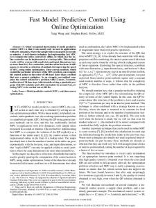
600 RES power production
� ′ ′ cu (k + j) u(k + j) + cz z(k + j) ,
subject to storage model (5); constraints (6), (7), (8); constraints (10); S · Pi (k + j) + s ≤ σi (k + j) ∀i;
500
400
(11) Power [kW]
J(xbk )
T −1 � X
300
200
100
xb (k|k) = xb (k),
0 0 1 2 3 4 5 6 7 8 9 10 11 12 13 14 15 16 17 18 19 20 21 22 23 24 time [hour]
where the column vectors cz and cu are given in the Appendix. We recall that the vector of disturbances profiles, w(k+j), ˆ is assumed to be known over the prediction horizon, for j = 0, . . . , T − 1. According to the receding horizon strategy, only the first element of the optimal sequence u(k) is applied. The optimization problem (11) is repeated at time k + 1, with the new measured/estimated state xbk+1|k+1 = xbk+1 . By doing so, an optimal feedback policy is designed. Note that in the MPC scheme, applied in this preliminary study, the controller makes its control decision by assuming that the predictions are correct (i.e. Certainty Equivalence).
RES power flows over 24 hours.
0.2 Spot energy prices 0.18 0.16
Price [Euro/kWh]
0.14 0.12 0.1 0.08 0.06 0.04 0.02 0
0 1 2 3 4 5 6 7 8 9 10 11 12 13 14 15 16 17 18 19 20 21 22 23 24 time [hour]
Fig. 2.
Spot energy prices over 24 hours.
110 Energy stored 100 90 80 70 Energy [kWh]
IV. S IMULATION RESULTS The proposed control strategy is investigated on a typical microgrid and simulation results are presented. This microgrid is in a grid-connected mode and comprises four DG units and photovoltaic panels. An energy storage is included, which is bounded between 10 kWh and 100 kWh and the maximal charge and discharge power are respectively 100 kW and −100 kW. We choose a sampling time of one hour. Simulations are performed over one day. Examples of renewable power production profiles and daily spot prices employed in the optimization routine are depicted respectively in Figure 1 and Figure 2. The microgrid is connected to the utility grid, so power can be bought or sold. The microgrid is allowed to reduce its controllable load preferred level from 10% to 50% in some given times of the day (from 10 am to 16 pm). The demanded power peak can be reduced up to 11%, as shown in Figure 6, leading to a cost reduction of 18%. The Figures 3, 5 and 4 depict, respectively, the energy stored, the power exchanged with the utility grid and the DG unit power production obtained by the MPC control strategy. It is shown that, starting from time 7, the MPC controller decides to turn on the DG units in order to meet the demand at minimum generation costs. In addition, the produced power is meaningfully increased at the times when there is both the highest RES power production and the highest demanded power (about from 10 am to 14 pm). For this reason, the storage device is kept at its maximum capacity during the previous hours and the most convenient amount of energy is bought from the utility grid. The RES power production is utilized either to fulfill the demand or to sell energy to the utility grid. We used ILOG’s CPLEX 12.0 to solve the MILP optimizations, which is an efficient solver based on the branch-and-
Fig. 1.
60 50 40 30 20 10 0
0 1 2 3 4 5 6 7 8 9 10 11 12 13 14 15 16 17 18 19 20 21 22 23 24 time [hour]
Fig. 3.
Stored energy over 24 hours.
bound algorithm [10]. When the branch-and-bound algorithm terminates, the solution is known to be globally optimal. The solution to each MILP problem took at most 6.1 seconds, a time much shorter than the sampling time of one hour. Thus, the computational burden can be affordable. V. C ONCLUSIONS AND F UTURE S TEPS In the paper we proposed a novel mixed integer linear approach on modeling and optimization of microgrids. We bring into account unit commitment, economic dispatch,
5453
50
Power [kW]
100
Power [kW]
0
100
Power [kW]
Power [kW]
realistic and less conservative approaches which ensure the stability and the feasibility of proposed MPC strategy.
DG unit 1 100
100
VI. A PPENDIX
0 1 2 3 4 5 6 7 8 9 10 11 12 13 14 15 16 17 18 19 20 21 22 23 24 DG unit 2
Eb 1
50 0
′
h
= C
b
′
′
Eb 3 = [1 − 1 1 − 1 0 0] h i ′ b E4 = C b − ε C b C b 0 0
0 1 2 3 4 5 6 7 8 9 10 11 12 13 14 15 16 17 18 19 20 21 22 23 24 DG unit 4
50 0
′
i
g Eb 2 = E2 = [0 0 1 − 1 1 − 1]
0 1 2 3 4 5 6 7 8 9 10 11 12 13 14 15 16 17 18 19 20 21 22 23 24 DG unit 3
50 0
− (C b + ε) C b C b − C b − C b
′
Eg1 = [T g − (T g + ε) T g T g − T g − T g ] h i ′ Eg3 (k) = 1 − 1 cP (k) − cP (k) cS (k) − cS (k)
0 1 2 3 4 5 6 7 8 9 10 11 12 13 14 15 16 17 18 19 20 21 22 23 24 time [hour]
′
Fig. 4.
Eg4 = [T g − ε T g T g 0 0]
DG units power production over 24 hours (ρ = 0.8).
where ε is a small tolerance (typically the machine precision) needed to transform a strict inequality constraint into a nonstrict inequality, since in MILP solving algorithm only nonstrict inequalities can be handled [9].
600 500
Energy exchanged with the utility grid with ρ=0.8 Energy exchanged with the utility grid with ρ=0
400
′
c 0 .{z . . 0}] F (k) = [1 . . 1} D1c (k) . . . DN c (k) | | .{z
300 Energy [kWh]
Ng
200
Ng
′
c f (k) = [1 − D1 (k) . . . − DN l (k) − D1c (k) . . . − DN c (k)]
100
′
0
. . 1} 0], . . 1} 1 1 cz = [1 | .{z | .{z Ng
−100
Ng
′
cu (k) = [0 . . 0} OM1 . . . OMN l 1 | .{z
−200 −300
Ng
0 1 2 3 4 5 6 7 8 9 10 11 12 13 14 15 16 17 18 19 20 21 22 23 24 time [hour]
c β1 (k)D1c (k) . . . βN c (k)DN c (k)].
Fig. 5. Purchased/sold energy over 24 hours. Notice the difference for different ρ’s.
R EFERENCES 800
Total demand Total demand with curtailments
700
600
Power [kW]
500
400
300
200
100
0
0 1 2 3 4 5 6 7 8 9 10 11 12 13 14 15 16 17 18 19 20 21 22 23 24 time [hour]
Fig. 6.
Curtailments over 24 hours (ρ = 0.8).
energy storage, sale and purchase of energy to/from the main grid, curtailment schedule. We assume perfect knowledge of the microgrid state, renewable resources production, future loads, and so on, which is useful to solve the optimization problem. Further, to cope with inevitable disturbances and forecast errors, we embed this into an MPC framework. Future work will focus on applying more realistic approaches to microgrid optimization, including state estimation and uncertainty modeling. Moreover we are currently studying
[1] N. Hatziargyriou, H. Asano, R. Iravani, and C. Marnay, “Microgrids,” IEEE Power & Energy Magazine, 2007. [2] G. Pepermans, J. Driesen, D. Haeseldonckx, R. Belmans, and W. D’haeseleer, “Distributed generation: Definition, benefits and issues,” Energy Policy, vol. 33, no. 6, pp. 787–798, 2005. [3] A. Siddiqui, C. Marnay, R. Firestone, and N. Zhou, “Distributed generation with heat recovery and storage,” Journal of Energy Engineering, vol. 133, no. 3, pp. 181–210, 2007. [4] F. Mohamed, “Microgrid modelling and online management,” Ph.D. dissertation, Helsinki University of Technology (Espoo, Finland), 2008. [5] A. Milo, H. Gaztanaga, I. Etxeberria-Otadui, E. Bilbao, and P. Rodriguez, “Optimization of an experimental hybrid microgrid operation: Reliability and economic issues,” in IEEE PowerTech Conference 2009, Bucharest, Romania, 2009, pp. 1–6. [6] J. Maciejowski, Predictive Control with Constraints. Harlow, UK: Prentice Hall, 2002. [7] L. Xie and M. Ilic, “Model predictive economic/environmental dispatch of power systems with intermittent resources,” in IEEE Power and Energy Society General Meeting, 2009. [8] R. Negenborn, M. Houwing, J. D. Schutter, and J. Hellendoorn, “Model predictive control for residential energy resources using a mixed-logical dynamic model,” in Proceedings of the 2009 IEEE International Conference on Networkin, Sensing and Control, ICNSC 2009, Okayama, Japan, 2009. [9] A. Bemporad and M. Morari, “Control of systems integrating logic, dynamics, and constraints,” Automatica, vol. 35, no. 3, 1999. [10] C. Floudas, Nonlinear and Mixed-Integer Programming Fundamentals and Applications. Oxford, UK: Oxford University Press, 1995.
5454