Energy Modeling of Processors in Wireless Sensor Networks based

Energy Modeling of Processors in Wireless Sensor Networks based on Petri Nets Ali Shareef, Yifeng Zhu∗ Department of Electrical and Computer Engineering University of Maine, Orono, USA Email: {ashareef, zhu∗ }@eece.maine.edu Abstract Power minimization is a serious issue in wireless sensor networks to extend the lifetime and minimize costs. However, in order to gain an accurate understanding of issues regarding power minimization, modeling techniques capable of accurately predicting energy consumption are needed. This paper demonstrates that Petri nets are a viable option of modeling a processor. In fact, this paper shows that the Petri nets’ accuracy surpasses a Markov model utilizing supplementary variables to account for constant delays.

1

Motivations

Wireless sensor networks are becoming increasingly prevalent in a wide range of areas from surveillance [6] to monitoring temperature, humidity, and other environmental parameters [12, 10]. Wireless sensor network are usually comprised of nodes powered by batteries in locations where maintenance access may be difficult. Minimizing energy consumption in these networks would go a long ways toward extending the lifetime of the network and increasing the usability. However, in order to obtain a thorough understanding of the energy consumption characteristics in these networks, accurate modeling methods need to be developed. Although the primary energy consumption in wireless sensor networks is for communication [2], the processor also serves a key role and there is a need to examine the energy characteristics of the embedded processors of these sensor nodes. A sound method of modeling provides a stable platform upon which the energy characteristics of innovative technology can be analyzed. One example of this is the capability of processors to power down to a low power mode after some time of no activity, which we will refer to as the Power Down Threshold. However, once powered down, the processor requires time Power Up Delay to reach operating mode again. In this paper, we compare two different processor models: a Markov chain and a Petri net against software simu-

lation. We show that the Petri net model is more accurate than the Markov chain. Section 2 introduces the use of both Markov models and Petri nets. Section 3 presents related work. Section 4 develops a model of a processor using a Markov model and a Petri net. Section 5 compares the results obtained by the simulation, Markov model, and Petri net, and Section 6 concludes this paper.

2

Introduction to the use of Markov Models, Petri Nets, and Software Simulation

Markov models have long been used to model systems dealing with exponentially distributed arrival and service rates. Markov models are composed of event chains where the likelihood of a system being in a particular state is independent of being in any other state. We can see how this restriction limits the usefulness of this method. Petri nets, on the other hand, are far more useful than Markov models. Initially Petri nets were based on Markov models, but since then, features of Petri nets’ have been extended over the years that has blurred these similarities. Unlike Markov models, Petri nets are a simulation based approach. Petri nets can be thought of as a directed graph of nodes and arcs which are called places and transitions respectively. With Markov models, closed form equations can be derived that can be used to provide analysis about the modeled systems. Petri nets require that the modeled system be simulated for extended periods of time so that the steady state probability of the system is reached. Computer program such as TimeNet 4.0 [13] are available that can assist in creating and simulating Petri nets.

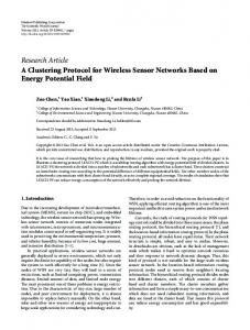
Figure 1. Example of Petri Net Figure 1 depicts a simple Petri net that contains two places P 0 and P 1 and a transition T 0. When a token exists in the input place of a transition as shown in P 0, this enables

the transition. When a transition is enabled, it fires according to user specified timing characteristics for that transition. When a transition fires, the token in the input place is removed and placed in the output place of the transition. In this case, the token in place P 0 is moved to place P 1. In this way, the operation of a system can be modeled and simulated. Statistical analysis of the average number of tokens in a particular place determines the steady state probability of the system being in that state. However, perhaps the most accurate method of modeling is through the use of software simulation where virtually anything can be programmatically modeled. Like Petri nets, software simulations are also repeated many times until the average behavior of the system can be achieved. A Markov chain can be used to construct analytical equations describing the average behavior of the system. However, mathematical difficulties that limit the usability of Markov models make simulation all the more appealing. On the other hand, the problem with simulation is that as the simulated system become more and more complicated, so does the software model of the system. This in turn results in increasing development, modification and testing time. Petri nets, on the other hand, can be constructed easily due to their graphical nature. The primary difference between the simulation, Markov, and Petri net model is that the Markov model utilizes a high level of abstraction. Whereas, the simulation and Petri net can be used to model at a much lower level closer to the actual hardware implementation. This enables the simulation and Petri net to account for the variations in the behavior of the processor [9].

3

Related Work

4

Evaluation of CPU with Markov and Petri Net

4.1

Modeling Energy Consumption CPU using a Markov model

Intrinsically, embedded systems operating in a wireless sensor network offer great potential for power minimization. Generally the level of computation required is low, and usually interspersed with communication between other nodes in the network. The power consumption of the CPU can be minimized by moving to a low power mode and conserving energy when it is not directly involved in any computation. There are two forms of workload generators that can be used to simulate workload for an application. One type is known as the closed workload model where a new task will not arrive until the current task has been completed. The other is known as the open workload model in which the tasks arrive independent of the state of the current task. Closed workload generators are best suited for modeling tasks that occur at set intervals. Open workload generators, on the other hand, are suited for tasks that are interrupt driven. Both workload generators are used depending upon the application. We will implement an open workload generator. In Figure 2 the CPU “powers up” (pu ) from a low power sleep mode when jobs begin arriving. The Markov model depicts the various increasing states (p01 , p02 , p03 , etc) the CPU enters as the number of jobs increase as given by the arrival rate λ. The CPU services the jobs at rate μ and strives to move the CPU to lower states and eventually to the idle state pi . If the processor remains in the “idle” state for some time interval greater than some threshold (Power Down Threshold), the CPU moves back to the standby state. λ

There have been many methods that have been proposed for modeling embedded systems to study energy characteristics. For example, Lee et al in [9] use energy measurements of instruction execution with regression analysis to derive equation that model energy consumption. Although this method achieves a high level of accuracy, this method can only be applied to computing energy during instruction execution. Energy consumption due to hardware interrupts is not accounted for. For example, the power up energy consumption is not linked with any instructions and hence cannot be modeled using this method. Coleri et al [3] have demonstrated the use of a Hybrid Automata to model TinyOS and hence the resulting power consumption of the nodes. Models based on finite state machines have been proposed in [8]. Although [11] discuss the use of Petri nets to model a single processor utilizing real-time scheduling, we have not found any literature that discusses the use of Petri nets to model energy consumption.

of

pi

λ

p01

idle

μ

p02 μ

e − λD

λ

λ

λ

p0n

...

μ

μ

μ

e − λD λ D

e λD

ps

standby

λ

pu

powerup

...

(λD ) n −1 ( n − 1)!

...

Figure 2. Birth-Death Process of CPU Jobs. In this example, we make the following assumptions: 1. The request arrivals follow a Poisson process with mean rate λ. 2. The service time is exponentially distributed with mean μ1 . 3. The CPU enters the standby state (ps ) if there are no more jobs to be serviced for a time interval longer than T (Power Down Threshold).

4. The power up process takes a constant time D (Power Up Delay). The CPU transition process consists of a mix of deterministic and exponential transitions. While all transitions shown as solid lines in Fig. 2 follow exponential time distributions, the transition from idle to standby is deterministic. The CPU enters the standby state after idling for a constant time threshold T . This power down transition depends on its history and is not memoryless. Accordingly, the CPU transitions can not be modeled directly as a Markov process. Using the method of supplementary variables proposed in [4], we derive an alterative set of state equations to approximate the effects of constant delays in stationary analysis. Let X = [x1 , x2 ] denote two age variables, representing how long a deterministic transition has become enabled [5]. And let Pi (x1 ) and Pu (x2 ) be the age density functions with respect to x1 in the idle state and with respect to x2 in the power up state, respectively. The state equations for this mixed transition process can be derived by the inclusion of the supplementary variable X. The deterministic transition from the idle state to the standby state can be modeled as below.  T Pi (x1 )dx1 (1) pi = 0

d Pi (x1 ) dx1 Pi (0) Pi (T )

= −λPi (x1 )

(2)

= μp01 = λps

(3) (4)

where Pi is an exponential function with coefficient λ. The deterministic power up process can be modeled as below.  D Pu (x2 )dx2 (5) pu =

We define the generating function of p0,n (n = 1, 2, . . .) as G0 (z) =

(6)

= λps

(7)

Thus we get G0 (1) =

(λ + μ)p01 (λ + μ)p0n

= λpi + μp02 + e Pu (0) = λp0,n−1 + μp0,n+1 + e−λD ∞ 

1 =

(λD)n−1 Pu (0) (n − 1)!

ps =

1−ρ eλT + (1 − ρ)(1 − e−λD ) + ρλD

(8)

for n ≥ 2(9)

p0,n + pi + ps + pu .

pi

=

λ λT e ps μ (eλT − 1)ps .

(11)

pu =

eλT

(1 − ρ)(1 − e−λD ) . + (1 − ρ)(1 − e−λD ) + ρλD

=

(1 − e−λD )ps .

(18)

And the utilization is G0 (1) =

ρ(eλT + λD) . + (1 − ρ)(1 − e−λD ) + ρλD

eλT ∞

(19)

Let L(z) = n=1 np0n z n , then L(1) is the total number of jobs in the system. ∞ 

L(z) =

d = z dz

np0n z n

∞ 

P0n z

n

n=1

d G0 (z) dz

(20)

Incorporating equation 15 into 20, we can get the total number of jobs in the system as follows. L(1) =

ρ eλT + 12 (1 − ρ)λ2 D2 + (2 − ρ)λD (21) 1 − ρ eλT + (1 − ρ)(1 − e−λD ) + ρλD

According to Little’s Law, the average latency for each job is L(1) τ= . (22) λ The total running time is

(12) T

From equations (5), (6), and (7), we have pu

(17)

(10)

From equations (1), (2), (3), and (4), we can get =

(16)

where ρ = μλ . Consequently,

= z

n=1

p01

 λps  λT e + λD . μ−λ

Substituting equations (11), (12), (13), (14) and (16) into the normalization equation (10) gives

In addition, when the system is stable, we have −λD

(14)

We multiply equation (8) by z and equation (9) by z n , add from n = 1 to ∞, use equations (7), (11), (12) (14), and get   λzps eλD(z−1) − 1 z . (15) G0 (z) = eλT + μ − λz z−1

n=1

= −λPu (x2 )

p0,n z n .

n=1

0

d Pu (x2 ) dx2 Pu (0)

∞ 

(13)

= =

N + L(1)τ λ N + L(1)2 λ

(23)

where N is the total number of jobs. Thus the total energy consumption is E

=

(pi Pidle + ps Pstandby + pu Ppowerup + G0 (1)Pactive )

N + L(1)2 λ

(24)

where Pidle , Pstandby , Ppowerup and Pactive are the power consumption rate in the idle, standby, powerup and active states (p01 , p02 , etc), respectively.

4.2

CPU Energy Modeling using a Petri Net

As was shown in the last section, the development of a Markov model for even a simple CPU is mathematically rigorous and cumbersome especially when dealing with deterministic transitions. Any slight modifications to the model will entail that the equations be re-derived again. Petri nets on the other hand offer a more flexible approach.

Figure 3. Petri net model of CPU

Transition AR T1 T2 SR P DT T5 T6 PUT

Firing Distribution Exponential Instantaneous Instantaneous Exponential Deterministic Instantaneous Instantaneous Deterministic

Delay Arrivals − − ServiceRate P DD − − PUD

Priority NA 4 1 NA NA 2 3 NA

Table 1. CPU Jobs Petri Net Transition Parameters Fig. 3 shows an Extended Deterministic and Stochastic Petri Net (EDSPN) [1] modeling a CPU as the Markov model described earlier. The Petri net models a CPU that starts from some “stand by” (Stand By) state and moves to an “ON” state (CPU ON) when jobs are generated. The CPU remains in the “ON” state so long as there are jobs in the CPU buffer. If there are no jobs in the CPU buffer, after

some time interval the CPU moves to the “stand by” state to conserve power. The model uses an open workload generator because when transition T 1 fires to deposit a task in the CP U Buf f er, a token is moved back to place P 0 which enables transition Arrival Rate and allows another task to be generated. Table 1 lists the parameters of all the transitions in the Petri net. The CPU is simulated by executing the Petri net using the following steps: 1) Jobs are generated in place P 1, when transition Arrival Rate fires randomly in the interval [0, 1] using an exponential distribution. The token in the place P 0 is moved to P 1 and enables T 1. 2) Transition T 1 is an immediate transition and fires as soon as it is enabled. Also since, T 1 has the highest priority, it will fire before any other immediate transition if multiple immediate transitions are enabled at once. When T 1 fires, the token is removed from P 1 and three tokens are generated. One is deposited in place P 0, one is deposited in place P 6, and one is deposited in the place CP U Buf f er. Initially, the CPU is in the Stand By mode. However, when a job arrives and a token is deposited in place P 6, transition T 6 is enabled. 3) When T 6 fires, the two tokens from Stand By and P 6 are removed and two tokens are then generated. One is placed in place P ower U p and one is placed in P 6. The CPU has now moved to a powering up state. Transition P ower U p Delay is now enabled with a token in P ower U p and in P 6. 4) Since transition P ower U p Delay has a deterministic delay, the transition fires after a fixed interval, and a token is deposited in place CP U ON . The CPU is now ON and ready to process events. 5) Remember that when T 1 fired, a token was placed in the CP U Buf f er, this token, the token in CP U ON , and the token in place Idle enables transition T 2. When it fires, the system is now in the processing state. With a token in Active, the transition Service Rate is enabled. 6) After Service Rate fires, the token is removed from Active and placed in Idle. 7) In the event that another task arrives while the system is still ON and processing other tasks, a token will be deposited in P 6 and CP U Buf f er. When the CPU is already ON, having a token in P 6 will enable T 5 which will fire immediately, and a single token will be placed in CP U ON . This is necessary because tokens cannot be allowed to accumulate infinitely in any place. 8) The token that was added to the CP U Buf f er will remain there until the CPU is idle as determined by a token in Idle. All jobs that arrive while the CPU is ON will cause the Petri net to cycle through steps 7 and 8. 9) However, in the event that the job arrival rate is very slow, the CPU will power down and move to the Stand By state. Note that when there is a token in CP U ON and no tokens in Active and CP U Buf f er, transition P ower Down T hreshold becomes enabled.

The small circle at the ends of the arcs from Active and CP U Buf f er specify this inverse logic. Since P ower Down T hreshold is a transition with deterministic delay, it will fire after a specified period as given by the value P DD, and the token from CP U ON will be removed and transferred to Stand By. By computing the average number of tokens in places during the simulation time results in the “steady state percentage” of time the CPU spends in the corresponding state. For example, the average number of tokens in CP U ON will indicate the percentage of time the CPU was on. The average number of tokens in P 7 will indicate the steady state percentage of time that the CPU was “powering up.” The percentages are determined by the system parameters Arrival Rate, Service Rate, P ower U p T hreshold, and P ower Down T hreshold delays. Once the percentages are obtained, they can be used to compute the total energy consumption of the system over time as given in Equation 25. T otalEnergy

=

(PStandby × P WStandby + PT imeP oweringU p × P WP oweringU p + PIdle × P WIdle + PT imeActive × P WActive ) × T ime (25)

5

Comparison between Simulation, Markov Models and Petri Net performance

In order to determine the feasibility of Markov models and Petri nets for modeling the behavior of a CPU, this section will compare them together. An event simulator written in Matlab was used to simulate the CPU repeatedly over multiple iterations until the steady state percentages for the desired states was obtained. Equation 25 was used to compute the total energy. The simulation will be used as a benchmark against which the performance of the Markov model and Petri net will be compared. The power parameters of the P XA271 Intel Processor as given in [7] were used to provide realistic analysis.

State Standby Idle Powering Up Active

Power Rate (mW) 17 88 192.442 193

Table 3. Power Rate Parameters for the PXA271 CPU (mW)

the Stand By state or “sleeps” to conserve power. When this happens, when the next job arrives, the CPU must transition to the P ower U p state where it spends time “waking up” (in the process consuming more energy) before it is able to service another job. Figure 4 indicates that both the Markov model and Petri net predict steady state percentages that are close to the simulation results. In fact, as Table 4 indicates, the difference between the Markov model and simulation is less than the difference between the Petri net and simulation. However, as we can see from Table 4 that as the Power Up Delay becomes larger, the performance of the Markov model begins to suffer. Power Up Delay (Sec) 0.001 0.3 10.0

Avg. Sim-Markov 0.338 4.182 116.788

Avg. Sim-PN 0.351 1.677 16.046

Avg. Markov-PN 0.076 3.338 103.077

Table 4. Δ Steady State Percentages (%) Estimates for Varying Power Up Delay

Figure 5 reveals the energy consumption characteristics of the CPU as the Power Down Threshold increases. It is obvious that as the CPU spends more time in the Idle state which has a higher power consumption rate than the Stand By mode, will result in increasing power consumed. 90 Idle Standby Power Up Active

80

1000 sec 1 per sec .1 per sec

Table 2. Simulation Parameters Figure 4 compares the behavior of the CPU as predicted by the simulator, the Markov model, and the Petri net when the Power Up Delay is fixed to 0.001 sec while the Power Down Threshold is varied. The solid line represents the simulator, the dashes with squares the Markov model, and the dashes with circles the Petri net. Since an open workload generator is being used, jobs arrive randomly in an interval. If the time between jobs exceeds the Power Down Threshold, then the CPU moves to

70 Percentage of time (%)

Total Simulated Time Arrival Rate Service Rate

60 50 40 30 20 10 0 0

0.1

0.2

0.3

0.4 0.5 0.6 0.7 Power Down Threshold (Sec)

0.8

0.9

1

Figure 4. Comparison between performance of Simulation, Markov Models, and Petri Nets for Power Up Delay of 0.001 sec.

0.001 sec in Table 4 and 5, the performance of the Markov model is better than the Petri net. If an effective method of modeling constant delays in Markov chains can be derived, the Markov model may very well become the modeling method of choice.

50

45

Energy (Joules)

40

35

30

References

25

20 Simulation Markov Petri Net

15

10 0

0.1

0.2

0.3

0.4 0.5 0.6 0.7 Power Down Threshold (Sec)

0.8

0.9

1

Figure 5. Energy Consumption Comparison between Simulation, Markov Model, and Petri Net for Power Up Delay of 0.001 sec. Power Up Delay (Sec) 0.001 0.3 10.0

Avg. Sim-Markov 0.154 1.558 24.866

Avg. Sim-PN 0.166 0.298 1.285

Avg. Markov-PN 0.037 1.401 25.411

Table 5. Δ Energy Consumption (Joules) Estimates for Varying Power Up Delay

Table 5 indicates that the difference in energy prediction between the simulation, Markov model and Petri net is almost the same. However, as the Power Up Delay begins to increase, we see that the effects of the deviating steady state percentages negatively effect the energy predictions of the Markov model. The approximation made for the effects of the constant delays in the Markov model is unable to account for the increasing constant delays and results in erroneous prediction for the Markov model.

6

Conclusion

The experimental results indicate that the Petri net is a better method of modeling processors than using a Markov model. This is due to the fact that a Markov model can only account for arrival and service rates that follow an exponential distribution. Markov models cannot handle fixed deterministic rates. Petri nets are also very easy to implement, and the complicated derivations of Markov models can be avoided. Any changes to the model can be made easily to a Petri net, while the Markov model will require re-derivation of the equations. However, the drawbacks to Petri nets is their long simulation time that is required before the percentages stabilize. Evaluating a Markov models means just evaluating an analytical expression. An interesting point to note is that when the constant delays are small such as when the Power Down Delays is

[1] TimeNET 4.0 A Software Tool for the Performability Evaluation with Stochastic and Colored Petri Nets, User Manual. [2] U. Cetintemel, A. Flinders, and Y. Sun. Power-efficient data dissemination in wireless sensor networks. In MobiDE, September 2003. [3] S. Coleri, M. Ergen, and T. J. Koo. Lifetime analysis of a sensor network with hybrid automata modeling. In WSNA ’02: Proceedings of the 1st ACM international workshop on Wireless sensor networks and applications, pages 98–104, New York, NY, USA, 2002. ACM. [4] D. R. Cox. The analysis of non-markovian stochastic processes by the inclusion of supplementary variables. Proceedings Cambridge Philosophical Society, 51(3):433–441, 1955. [5] R. German. Transient analysis of deterministic and stochastic petri nets by the method of supplementary variables. In MASCOTS ’95: Proceedings of the 3rd International Workshop on Modeling, Analysis, and Simulation of Computer and Telecommunication Systems, pages 394–398, Washington, DC, USA, 1995. IEEE Computer Society. [6] T. He, P. Vicaire, T. Yan, Q. Cao, G. Zhou, L. Gu, L. Luo, R. Stoleru, J. A. Stankovic, and T. F. Abdelzaher. Achieving long-term surveillance in vigilnet. In INFOCOM. IEEE, 2006. [7] D. Jung, T. Teixeira, A. Barton-Sweeney, and A. Savvides. Model-based design exploration of wireless sensor node lifetimes. In Proceedings of the Fourth European Conference on Wireless Sensor Networks. EWSN 2007, Jan. 2007. [8] S. Kellner, M.Pink, D. Meier, and E.-O. Blass. Towards a realistic energy model for wireless sensor networks. In Proceedings of IEEE Fifth Annual Conference on Wireless On demand Network Systems and Services, pages 97–100, January 2008. [9] S. Lee, A. Ermedahl, S. L. Min, and N. Chang. An accurate instruction-level energy consumption model for embedded risc processors. In Proceedings of the ACM SIGPLAN Workshop on Languages, Compilers, and Tools for Embedded Systems, pages 1–10, June 2001. [10] A. Mainwaring, J. Polastre, R. Szewczyk, D. Culler, and J. Anderson. Wireless sensor networks for habitat monitoring. In ACM International Workshop on Wireless Sensor Networks and Applications (WSNA’02), Atlanta, GA, September 2002. [11] M. Naedele. Petri net models for single processor real-time scheduling. [12] J. Polastre, R. Szewczyk, A. Mainwaring, D. Culler, and J. Anderson. Analysis of wireless sensor networks for habitat monitoring. In Wireless sensor networks, pages 399–423, Norwell, MA, USA, 2004. Kluwer Academic Publishers. [13] A. Zimmermann, M. Knoke, A. Huck, and G. Hommel. Towards version 4.0 of TimeNET. In 13th GI/ITG Conference on Measurement, Modeling, and Evaluation of Computer and Communication Systems (MMB), pages 477–480, Mar. 2006.