Energy savings in Wireless Mesh Networks in a time-variable context

Noname manuscript No. (will be inserted by the editor)

Energy savings in Wireless Mesh Networks in a time-variable context Antonio Capone · Filippo Malandra · Brunilde Sansò

Abstract Energy consumption of communication systems is becoming a fundamental issue and, among all the sectors, wireless access networks are largely responsible for the increase in consumption. In addition to the access segment, wireless technologies are also gaining popularity for the backhaul infrastructure of cellular systems mainly due to their cost and easy deployment. In this context, Wireless Mesh Networks (WMN) are commonly considered the most suitable architecture because of their versatility that allows flexible configurations. In this paper we combine the flexibility of WMN with the need for energy consumption reduction by presenting an optimization framework for network management that takes into account the trade off between the network energy needs and the daily variations of the demand. A resolution approach and a thorough discussion on the details related to WMN energy management are also presented.

70 % of overall telecommunications network energy expenditures and this percentage is expected to grow in the next decade [5,6]. An important part of the energy consumption is given by the wireless part of the access and it has been estimated that the base stations represent 80% of the total wireless consumption [7]. It follows that being able to minimize base station consumption represents an important green networking objective.

1 Introduction

As a matter of fact, the resources of Wireless Access Networks are, for long periods of time, underemployed, since only a few percentage of the installed capacity of the Base Stations (BS) is effectively used and this results in high energy waste [9,10]. In WMNs also, network devices are active both in busy hours and in idle periods. This means that the energetic consumption does not decrease when the traffic is low and that it would be possible to save large amounts of energy just by switching off unnecessary network elements.

Green Networking consists of a rethinking of the way networks are built and operated so that not only costs and performance are taken into account but also their energy consumption and carbon footprint. It is quickly becoming one of the major principles in the world of networking, given the exponential grow of Internet traffic that is pushing huge investments around the world for increasing communication infrastructures in the coming years. In fact, the Information and Communication Technology (ICT) sector is said to be responsible for 2% to 2.5 % of the GHG annual emission [1, 2,3] as it generates around 0.53Gt (billion tonnes) of carbon dioxide equivalent (CO2 e). This amount is expected to increase to 1.43GtCO2 e in 2020 (data from [4]). Among Internet related networking equipment, it is the access the one with the major impact in energy expenditures. It has been estimated that access networks consume around A. Capone and F. Malandra Politecnico di Milano, Piazza Leonardo da Vinci, 32, Milano, Italy B. Sansò Ecole Polytechnique de Montreal, 2900, boul Edouard-Montpetit, Montreal, Canada.

An increasingly popular type of wireless access are the so-called Wireless Mesh Networks (WMNs) [8] that provide wireless connectivity through much cheaper and more flexible backhaul infrastructure compared with wired solutions. The nodes of these dynamically self-organized and self-configured networks create a changing topology and keep a mesh connectivity to offer Internet access to the users. Obviously, the use of wireless technologies also for backhauling can potentially make the issue of energy performance even more severe if appropriate energy saving strategies are not adopted.

The focus of our work is to combine the versatility of Wireless Mesh Networks with the need of optimizing energy consumption by getting advantage of the low demand periods and the dynamic reconfigurations that are possible in WMNs. We propose to minimize the energy in a time varying context by selecting dynamically a subset of mesh BSs to switch on considering coverage issues of the service area, traffic routing, as well as capacity limitations both on the access segment and the wireless backhaul links. To reach our objective, we provide an optimization framework based on mathematical programming that considers traffic demands for a set of time intervals and manages the energy consumption of the network with the goal of making it proportional to the load.

2

Energy management in wireless access networks have been considered very recently in a few previous works [11,9,12,2, 13,14,15,1] (see Section 2 for a detailed review of the state of the art). In this paper, we present a novel approach for the dynamic energy management of WMNs that provides several novel contributions: – We consider not only the access segment but also the wireless backhaul of wireless access networks; – We combine together the issue of wireless coverage, for the access segment, and the routing, for the backhaul network, and optimize them jointly; – We explicitly include traffic variations over a set of time intervals and show how it is possible to have energy consumption following these variations; – We provide a rigorous mathematical modeling of the energy minimization problem based on Mixed Integer Linear Programming (MILP), and solve it to the optimum. The paper has been structured as follows. After a brief survey of the literature concerning general and wireless Green Networking in ICT in Section 2 we present the system model and preliminary descriptions in Section 3. The optimized modeling approach for system management is introduced in Section4. The resolution approach and a thorough results analysis are presented in Section 5. Section 6 concludes the paper.

2 Related work The problem of energy consumption of communication networks and the main technical challenges to reduce it have been presented in the seminal work by Gupta and Singh [16]. Several proposals to reduce networks foot print as well as energy consumption have appeared in the last few years, considering both wireless and wired networks [17,18,19,20,21, 22,23,24]. Good overviews of the research on green networking and methodological classifications are given in [25,26] where different methods adopted in the literature for both wired and wireless networks are surveyed. In what follows, we focus on wireless networks only. The literature in wireless device energy optimization is quite large, given the limitation of the battery and the natural restrictions of the wireless medium. In fact, energy consumption has always been a concern for wireless engineering given the mobility of users that require portability, which makes coverage and battery life issues a true challenge. There is, indeed, a large body of work on energy-efficiency for devices and protocols for cellular, WLAN and cellular systems (see [27], for an excellent survey). However, the interest for energy optimization of the wireless infrastructure has only picked up in recent years given the explosion in Internet wireless applications. There has been some work to compare wireless and wireline infrastructure consumption. For instance, let us mention [16] where the energy cost (W h/Byte) for a transmission over the Internet was compared to the cost of the same transmission in a wireless context (for instance Wi-Fi 802.11b).

Antonio Capone et al.

Wireless resulted more efficient by a small factor with omnidirectional antenna and it was found that the factor could be improved using directive antennas. Our main concern, however, is wireless network management for which we have found articles that deal either with Wireless Local Area Networks (WLANs) or with traditional cellular access networks. In WLANs, we mention the work of [11] that presented strategies based on the resource on-demand (RoD) concept. [9] proposed an analytical model to assess the effectiveness of RoD strategies and [12] shows management strategies for energy savings in solar powered 802.11 wireless MESH networks. Concerning cellular access networks, [2] considered the possibility of switching off some nodes but without considering traffic variations, which can produce substantial savings given that cellular systems are generally dimensioned for peak traffic conditions. [14], on the other hand, studied deterministic traffic variations to characterize energy savings and showed that they can be around 25 - 30% for different types of regular cell topologies. Another energy management study is provided by [13] where it is shown that the on-off strategy for UMTS BS is feasible in urban areas. [15] considered a random traffic distribution and dynamically minimized the number of active BSs to meet the traffic variations in both space and time and [1] presented an optimization approach for dynamically managing the energy consumption. The differences of our work with the papers mentioned above is that the later deal exclusively with access networks while our goal is to manage the energy consumption of WMNs that use the wireless medium not only for the access segment but also for the backbone. The presence of the wireless backbone forces us to consider the routing of traffic from base stations (or mesh access points) to the mesh gateways (interconnecting the WMN to the wired network). This issue, in addition to the coverage aspects of the service area typical of the access segment, makes the problem of energy management in WMNs a combination of the problems considered so far for wired and wireless networks. To the best of our knowledge, this is the first paper proposing a network management framework aimed at optimizing the energy consumption of WMNs.

3 System model and problem description In this Section, we first present the physical and technological features of the system. Next, we describe the details of the traffic scenarios that will be essential to understanding the modeling issues. Finally we present the model that will be used as the basis for the energy efficient formulation and introduce the general approach to WMN energy management.

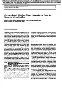
3.1 Description of the system The WMN architecture such as the one presented in Figure 1 is made up of fixed and mobile elements, namely Mesh

Energy savings in Wireless Mesh Networks in a time-variable context

INTERNET

3

index t

Starting

ending

duration (h)

pt

1 2 3 4 5 6 7 8

0 3 6 9 12 15 18 21

3 6 9 12 15 18 21 24

3 3 3 3 3 3 3 3

0.35 0.1 0.45 1 0.7 0.85 0.6 0.5

MU MAP MR

Table 1: Day division in time intervals and related level of congestion

Figure 1: Architecture of the network analysed 3.2 Traffic profiles

Routers (MR) and Mesh Users (MU). MRs could have different functions and features building up a variety of structures and architectures. A restricted part of the set of routers is used as gateway to other larger networks, typically the Internet. In particular, the so called Mesh Access Points (MAP) can communicate with the other routers with a radio communication channel and also have a fixed connection to the Internet. In what follows, the term Base Station (BS) will be used as a general term to design either MAPs or MRs. In our networks’ distribution system MRs and MAPs communicate through a dedicated wireless channel, each MU is connected to the nearest active base station and, through multi hop communications, to the Internet. The devices are all equipped with multiple network interfaces, so we can infer that the traffic in a given link does not affect closer links. The interference is not totally removed but it can be minimized installing directive antennas and adopting a smart frequency assignment algorithm as suggested in [28]. So every link between two base stations has a fixed bidirectional capacity. We also assume that this capacity does not depend on the distance and that a wireless link is possible between two MRs only if they have a distance to each other lower than a value called covering ray. Even if the modeling approach proposed is general and can be used with any wireless technology, we have focused our analysis on WiFi WMNs. The technology used among routing devices is assumed to be Wi-Fi 802.11/n with a nominal capacity of 450 Mbps and a covering ray of 450 metres. Concerning the communication between users and BSs, we suppose that the access technology is Wi-Fi 802.11/g with 54 Mbps. This access capacity has to be shared among all the MUs assigned to a given BS. A MU can be assigned to a MR if and only if it is inside a circular cell with the center at the BS and a ray of 250 metres. Note that the difference between the two mentioned rays is due to the use of directive antennas which allow to double the covering distance. Also assumed is a certain percentage of losses derived from the protocol OH that reduce the effective link capacities. The details on this issue will be given in subsection 5.2.

In [29] and [30] the characteristics of the traffic in Wireless Access Networks have been analyzed and it is shown how the traffic during the day can be split into intervals of equal length that we define ∆T . Since we want to optimize the energy consumption during the day in such a way as to make the consumption f ollow the demand as much as possible, it is important to assume a realistic traffic profile. For that, we have divided the day into eight intervals of three hours and have assigned a probability pt of test points requesting demand in each interval t that follows the traffic characteristics presented in [30] and [29]. The results are presented in Table 1. Moreover we used two different traffic profiles: – standard, with traffic randomly generated in the interval from 1 to 10 Mbps – busy, with a traffic request that varies between 8 and 10 Mbps.

3.3 A general approach to WMN energy management The general problem we are considering aims at managing network devices in order to save energy when some of the network resources, namely BSs and the links connecting them, are not necessary and can be switched off. Even if the specific implementation issues are out of the scope of this work, it is easy to see that an energy management strategy like the one we propose can be integrated with no difficulty in the network management platforms that are commonly adopted for carrier grade WMNs and that allow the centralized and remote control of all devices and the change of their configuration with relatively slow dynamics (hours) [31]. From an energy efficiency standpoint, there are several questions that should be answered concerning the deployment and operation of WMN. It is clear that in order to follow the varying demand, it is not enough to consider that some mesh BSs should be powered down. To have an effective energy management system, we must address the question of which base stations to select, how to guarantee that the requested QoS is maintained despite shutting down the equipment, how users are reassigned after shut down and how the initial coverage and network topology has an impact on energy savings and energy consumption.

4

Antonio Capone et al.

Given that an appropriate network planning provides the basis for an effective energy management operation, we now present the basic planning model introduced in [32] and explain how that model is modified to obtain a general framework for energy management. The idea of the model is that, given a set of TP (Test Points) representing aggregated points of demand and a set of possible BS sites decide where and what type of equipment to locate while satisfying the TP demand and minimizing costs. In more formal terms, let S be the set of the candidate sites (CS) to install routing devices like MRs or MAPs, I the set of test points and N a special node representing the Internet. The network topology is defined by two binary parameters: aij that is equal to 1 if a BS in CS j covers the TP i and bjl equal to 1 if CS j and in CS l could communicate through a wireless link. The traffic requested by TP i is denoted by di . Binary variables xij are used for the assignment of TP i to CS j, while zj are installation variables related to CSj. Additional binary variables are wjN , that show if a MAP is installed in CS j, and yjl that define if there is a wireless link between the two CSs j and l. The integer variable fjl represents the traffic flow on wireless link (j, l) while fjN is the flow from the MAP in CS j to the Internet. Given the above parameters and variables we can summarize the mathematical formulation as follows: X

min

(cj zjt + pj wjN )

(1)

j∈S

s.t.

X

xij = 1

∀i ∈ I,

(2)

∀i ∈ I∀j ∈ S,

(3)

two nodes exists only if they are both active (8) and neighbour (9). (10) imposes the assignment of a TP to the nearest active BS while (11) restricts the decision variables to take binary values. Note that the above is an optimal planning formulation that does not take into account the temporal variations of the demand nor the dynamics of the coverage that are necessary in an efficient operational energy management scheme. Thus, to create the energy management framework, the above model is modified as follows: – The objective function changes to recreate an energy efficient objective. – The main philosophy of the model changes as there are no longer Candidate Sites but rather installed Base Stations at particular sites that could be put down according to the variations in demand. – A dynamic assignment of users to coverage areas is enforced. – System parameters are modified to account for the temporal notion of the operation. – The decision variables reflect the fact that the equipment can be powered down at particular instants of time. – Constraints are added to relate the dynamic assignment with the state (on or off) of the equipment. 4 Optimized framework for energy management For simplicity, we first present a first optimal energy management model. Then, we introduce variations to the model that take into account different energy related elements that we want to study and that will be put into relevance in the analysis of the results.

j∈S

xij 6 zj aij X (flj − fjl ) +

4.1 An optimal energy management model

l∈S

+

X

di xij = fjN

∀j ∈ S,

(4)

flj − fjl 6 ujl yjl X di xij 6 vj

∀j, l ∈ S,

(5)

∀j ∈ S,

(6)

∀j ∈ S,

(7)

yjl 6 zj , yjl 6 zl

∀j, l ∈ S,

(8)

yjl 6 bjl

∀j, l ∈ S,

(9)

i∈I

i∈I

fjN 6 M wjN

li X

xij (i) + zj (i) 6 1 h

∀l = 1, ..., Li − 1, ∀i ∈ I, (10)

l

h=l+1

xij , zj , yjl , wjN ∈ {0, 1}

∀i ∈ I, ∀j, l ∈ S. (11)

Objective function (1) accounts for the total cost of the network including installation cost cj and costs pj related to the connection of a MAP to the wired backbone. (2) forces each TP to be assigned to one active CS that covers it (see (3)). (4) is a classical flow balance set of equations while (5),(6) and (7) are sets of capacity constraints for, respectively, links, routers and gateways. A wireless link between

The main idea of the model is to decide which elements of the network should be turned off and at what instants of time so that energy consumption is minimized and the demand is always satisfied. For this, the model must also convey the delicate balance between operation dynamics and user coverage. We assume that the network has been previously built, that Base Stations have been installed and that the site of the TPs is known in advance. Therefore, we propose the following mathematical notation. Sets: I

the set of TPs

T

the set of time intervals

S

the set of BS, being MRs or MAPs

G⊆S (i) Jh

the subset of BS that are MAPs (gateways) the subset of BSs covering TP i ordered by decreasing received power where h is the index of position inside the set

Input parameters:

Energy savings in Wireless Mesh Networks in a time-variable context

aij =

(

bjl =

(

1 0

X

if the TP i is covered by BS j otherwise

1 if a wireless link between BSs j and l is possible

dit

traffic request of TP i at time t,

ujl

capacity of the link between BSs j and l,

vj

access capacity BS j can offer to its TPs,

Li

number of BS covering TP i

ξj

power consumption of the device j ∈ S.

m

capacity of Internet access of the MAP

Decision variables: ( 1 if TP i is assigned to BS j at time t xijt = 0 otherwise ( 1 if BS j is active at time t zjt = 0 otherwise fjlt

flow between BSs j and l at time t

fj0t

flow from BS j to Node 0 at time t

zjt ξj ∆T

X

dit xijt = fj0t

∀j ∈ S, ∀t ∈ T

(15)

i∈I

(15) is the classical set of flow balance constraints. The first term represents the difference between the ingoing and the outgoing traffic in the links among BSs P that can
be of different type (MAPs or MR). The term i∈I dit xijt is the traffic supply of the device to its TPs. Finally, the last term fj0t represents the flow between the MAPs and the Internet, considered as special node 0. Capacity constraints There are several types of capacity constraints. Constraints (16) insure that the capacity of each node is respected whereas (17) refer to the capactiy of the link. (18), on the other hand, imply that the capacity of the Internet access of each MAPs must be m. dit xijt 6 vj

∀j ∈ S, ∀t ∈ T

(16)

∀j, l ∈ S, ∀t ∈ T

(17)

∀j ∈ G ⊆ S, ∀t ∈ T

(18)

i∈I

fljt + fjlt 6 ujl bjl zjt fj0t 6 m

Best assignment constraints

(12)

j∈S t∈T

We assume that the power consumption of our devices is constant during each interval of time and equal to the previously defined ξj . Therefore, the energy consumption of a given BS j is obtained by multiplying ξ by the activity time length and the decision variable that indicates if the BS is active. The total energy consumption is then obtained by summing up over all BS and all intervals of time considered. The objective will be to minimize (12). Assigment constraints There are two type of assignment constraints. (13) imposes that at each time interval every TP is assigned to a BS and (14) requires the BS assigned to be active and to cover the given TP. These are important constraints in energy management given that they relate a time-varying covering functionality with a time-varying BS operation.

xijt = 1

∀i ∈ I, ∀t ∈ T

(13)

xijt 6 zjt aij

∀i ∈ I, ∀j ∈ S, ∀t ∈ T

(14)

j∈S

Flow conservation constraints

+

X

We now explain each element of the optimal energy management model (P 1): The objective function

X

(fljt − fjlt ) +

l∈S

0 otherwise ( 1 if TP i is requesting traffic (dit > 0) at time t hit = 0 otherwise

XX

5

li X

xiJ (i) t + zJ (i) t 6 1 h

∀l = 1, ..., Li − 1,

l

h=l+1

∀i ∈ I, ∀t ∈ T

(19)

This set of constraints forces every TP to be assigned to the best active device. Binary constraints Finally, we have the constraints that impose binary values to the decision variables. xijt , zjt ∈ {0, 1}

∀i ∈ I, ∀j, l ∈ S, ∀t ∈ T

(20)

Summarizing model P 1 can be presented as follows: min (12) s.t. (13) to (20). 4.2 The covering-relaxed Problem We have also developed some variants of the proposed model presented above, not only to have a basis for comparison but also to be able to grasp some of the particular features of the energy management situation. The covering-relaxed model P 1 is obtained relaxing the assignment constraints of P 1. Let us focus on constraints (13): X j∈S

xijt = 1

∀i ∈ I, ∀t ∈ T

6

Antonio Capone et al.

This set of constraints imposes that every TP must be assigned to one and only one BS and, since (14) forces to assign a terminal to a device only if it is active and it covers it, we can derive that each TP is assigned to, and subsequently covered by, one active BS. We want to restrict the application field of the covering constraints only to active TPs and this will result in a lack of coverage of those terminals that are not active. Thus, the previous sets of constraints (13 and 14) are relaxed and replaced by the following: X

xijt = hit

∀i ∈ I, ∀t ∈ T

(21)

j∈S

kind of WMN

dimension (m)

tps

BS (MAPs)

small medium large

1000 1500 2500

60 130 240

16(2) 40(3) 64(5)

Table 2: Types of WMN used in our optimization analysis

– specific values of the technology used such as access capacity of the BSs, capacity of the wireless links, covering rays and so on; – a random traffic profile with a different level of congestion for each time interval. Once IG is applied, the resulting instance must have:

Then, P 1 can be defined as follows: min (12) s.t. (15) to (21). Since P 1 is a relaxation of P 1 its objective function will be a lower bound that would be used in the analysis of the results presented in the next Section.

4.3 Additional problem variations Two additional situations will be used for comparison purposes: one is the total absence of traffic, in which no traffic is requested from any of the TPs (dit = 0 ∀i ∈ I, ∀t ∈ T ) and another one in which all TPs are active and demanding the maximum amount of traffic (dit = 10Mbps ∀i ∈ I, ∀t ∈ T ). We call the first case the no-traffic problem P 10 and the second one, the f ull-traffic problem P 1f . The objective functions of these two cases will provide us with useful comparison bounds that will be discussed in the results Sections.

5 Resolution approach and results analysis To test our models and extract the most relevant information we first created an instance generator, then we produced a large set of instances that were optimized using AMPL and CPLEX. Followed the comparative results for the four variations of the problem.

5.1 Instance generation Generating feasible WMN instances is a delicate process since we need to use network topologies that can represent possible network deployments provided during the design phase. Thus, we developed an instance generator program (IG) in C++ that takes into account the following issues: – the topology, the dimension of the area analyzed and the numbers of TPs and BSs to place; – the architecture, in particular the placement of all devices according to certain controls;

– a random topology, according to certain constraints, – feasible assignments, – realistic values. The first item above refers to the fact that the topology and the architecture are generated randomly inside a predetermined area. The second one refers to the fact that each BS must be able to provide the TPs with the maximum traffic amount possible and the third one refers to the technologically feasible values assigned to the different input parameters. Moreover, specific controls are added to the random generation to insure network feasibility. 5.2 Input assumptions and parameter values All the optimization instances presented the following input values – R1 = 450m, is the covering ray for the communications between MRs or MAPs; – R2 = 250m, is the covering ray for the communications between a BS and the terminals associated to it; – vj = 40 Mbps, ∀j ∈ S, uij = 300 Mbps, ∀i, j ∈ S and m = 10 Gbps; – ξj = 15W if j is a MR and 18W if j is a MAP. Moreover, three different kinds of WMN were generated. Their features are portrayed in Table 2. The first column refers to the name that will be used throughout the analysis to identify the type of instance. The second corresponds to the size of a square area. The third is the number of TPs available in the instance. Finally, in the third column we have the number of installed BS (MR or MAPs), the MAPs being identified in parenthesis. We have generated 150 instances for each kind of WMN presented in Table 2 and all the mean results over the 150 instances will be shown in Table 3. To understand the table, we need to define some additional notation. Let β be the consumption of a WMN when all BS are active; c be the value of objective function (12); α the percentage of savings when compared with the consumption when all BS are active (α = 1 − c/β) and γ the total traffic requested by all terminals . By abuse of notation, we will also use the following subscript to refer to particular values:

Energy savings in Wireless Mesh Networks in a time-variable context

7

mean value of the parameters

14616 13535 6099

23400 23171 11845

1200

5904 5875 2751

Small WMN − Standard profile

θ (%) θ (%)

3252 6876 6036 52.956 58.699

6012 13627 12283 41.762 47.505

0 0

0.755 1.777

2.448 4.737

400

1501 3222 2883 45.414 51.157

200

large

0

γ (Mbps) c (Wh) c (Wh) α (%) α (%)

medium

y axis

Standard traffic small

MU MAP MR

1000

large

800

medium

600

β (Wh) cf (Wh) c0 (Wh)

small

0

200

800

1000

1200

5320 8985 8314 38.525 43.116

9843 16946 15915 27.579 31.984

0 0

0.565 1.739

1.834 3.771

MU MAP MR

400

Table 3: Numerical results of the optimization process

Small WMN − original problem (time interval 2) 1200

2461 4140 3866 29.877 34.511

(a)

1000

large

800

medium

600

small

y axis

θ (%) θ (%)

600

x axis 60 TP − 16 BS (2 MAP − 14 MR)

Busy traffic

γ (Mbps) c (Wh) c (Wh) α (%) α (%)

400

0

200

– t, the value at time interval t, (i.e. ct ), – f , the value in the full-traffic situation (i.e. cf ), – 0, the value in the no-traffic situation (i.e. c0 ).

0

200

400

600

800

1000

1200

x axis Active BS: 8 (MAP: 1 MR: 7)

(b)

1200

Small WMN − original problem (time interval 4)

600

800

1000

MU MAP MR

0

5.3 Energy performance and network topology

200

400

y axis

Also note that the underline will refer to the values associated to the covering-relaxed model. It is important to point out the difference between β and cf : the first is the consumption of a WMN without optimization, that is, the sum of all the installed BS consumption while the second is the consumption evaluated as the objective of problem P 1f , that is, the consumption in the optimized case when all TPs are active and demand the maximum value of traffic. It is then clear that while β depends solely on the number of BS, regardless of their location, cf is related to the TP demand and, therefore,depends on the network topology.

From Table 3 the first thing to point out is that the difference between β and cf is very low, around 2% for the small instances, 7% for medium ones and 1% for the large ones. This means that the instances are well generated and, in particular, that the total number of BSs is realistic. There are no unnecessary devices installed but all are used to guarantee the activity of the networks in the hypotheses of all terminals being active and generating the maximum amount of traffic (10 Mbps). Looking at the optimization gap values θ and θ given in the Table, one can see that for the small networks all solutions are optimal and that all gaps are under a tolerance

0

200

400

600

800

1000

1200

x axis Active BS: 10 (MAP: 2 MR: 8)

(c)

Figure 2: An example of small WMN represented first with all active devices, then in two different time intervals

8

Antonio Capone et al.

2500

MU MAP MR

1500 1000

y axis

1000

2000

1500

MU MAP MR

0

0

500

500

y axis

Big WMN − Busy profile 3000

Medium WMN − Busy profile

0

500

1000

1500

0

500

x axis 130 TP − 40 BS (3 MAP − 37 MR)

1000

2500

3000

(a) Big WMN − original problem (time interval 2) 3000

Medium WMN − original problem (time interval 2)

MU MAP MR

1500 0

0

500

500

1000

y axis

1000

2000

2500

MU MAP MR

1500

2000

x axis 240 TP − 64 BS (5 MAP − 59 MR)

(a)

y axis

1500

0

500

1000

1500

0

500

x axis Active BS: 18 (MAP: 1 MR: 17)

1000

2500

3000

(b)

Medium WMN − original problem (time interval 4) 3000

Big WMN − original problem (time interval 4)

MU MAP MR

MU MAP MR

1500 0

0

500

1000

500

y axis

1000

2000

2500

1500

2000

x axis Active BS: 36 (MAP: 3 MR: 33)

(b)

y axis

1500

0

500

1000

1500

x axis Active BS: 36 (MAP: 3 MR: 33)

(c)

0

500

1000

1500

2000

2500

3000

x axis Active BS: 62 (MAP: 5 MR: 57)

(c)

Figure 3: An example of medium WMN represented first with all active devices, then in two different time intervals

Figure 4: An example of a large WMN represented first with all active devices, then in two different time intervals

Energy savings in Wireless Mesh Networks in a time-variable context

threshold of 5% even for medium and large networks, which implies that these are problems that can be solved fairly well with direct optimization methods. Regarding the value of α and α, that is, the mean energy gains obtained when solving the main optimization problem or the covering relaxed problem, we can see that, for the standard traffic we can easily reach 40% of savings whereas for the heavy traffic the savings are closer to 30%. In all the cases, there is at least a 5% difference in savings with the solution of the covering relaxed problem. To portray the network topologies found from the optimization model, we can see the three network examples in Figures 2,3 and 4. Figures 2-a, represents the initial small network that represents 60 TPs and 16 installed BSs, we can see that when the optimization model is applied, the topology is reduced to 8 BS for the second interval, which has low demand, and to 10 BS for the fourth interval, which has high demand ( see figures 2-b and 2-c, respectively). The same trend can be seen by examining figures 3 and 4. One can see that in all the cases, the networks are less connected for the second and fourth intervals, thus requiring fewer resources. It can be appreciated that in all cases, the topology presents more links in the fourth than in the second interval but fewer links than the distribution system, showing the difference it makes to optimize the energy consumption. A more detailed view of the energy management features and its relationships with network topology can be appreciated by inspecting Tables 4, 5 and 6. The Tables present the minimum, average and maximum number of base stations and MAPs found for each interval of time, over the 150 instances that were run, for normal and heavy traffic and for the three types of network sizes, respectively. In the Tables we have bolded the results for which the upper bound (on the number of BS or MAPs) is equal to the initial problem. We can see that, with respect to the BS of the small network (see Table 4) only two instant of times (t = 4, 6) in the busy case present the maximum number of BS up. Remarkably, in all the other instances and cases, there is a considerable number of BS shut down. For the large network (Table 6), the situation occurs in just one interval, for (t = 4), also for the busy case. However, for the medium size network (see Table 5),no interval or case, among the 150 instances produced with different demand levels needed the maximum number of base stations. This shows the power of optimizing the energy management. With respect to the MAP, the opposite occurs: in almost all intervals and cases the maximum number of MAPs is obtained, except for interval (t = 3) for the large network, heavy traffic and covering relaxed problem in which a lower number of MAPs were installed in the worst case. 5.3.1 Energy profiles In Figures 5, 6 and 7 the mean consumption profiles per interval over all the small, medium and large network instances, respectively, are provided. The subfigures (a) represent the case for standard demand and (b) for busy demand. In every one of those figures one can appreciate four different

9

consumption levels: that for the original problem P 1, the full traffic problem P 1f , the covering-relaxed problem P 1 as well as the no traffic one P 10 . The full-traffic consumption, that is to say the energy necessary to feed the WMN with all terminal active and demanding for the maximum value of traffic (γ), is the upper bound for the consumption in all the cases. There are, however, two lower bounds, the one derived by the relaxation of the covering constraint and the one related to the absence of traffic. What is interesting is that these two bounds appear at different intervals of time. For the cases with standard demand, the value of the objective function of the coveringrelaxed problem is the lower bound for the first three and the last intervals, all of which present a traffic demand below 50%. The value of the energy objective for problem P 10 , which represents the case in which there is absence of traffic, is, on the other hand, the lower bound for all the other intervals. For the cases with busy demand, the covering-relaxed problem will be the lower bound only for the first two intervals. In all cases, during the intervals of normal operation, the covering-relaxed problem tended to produce the same optimization result than the original case. This means that when the demand is close to the nominal one, there is no gain in relaxing the covering constraints. On the other hand, when the demand is low, relaxing that constraint can yield important gains even when compared with the energy optimized problem. In all the cases the optimization model produces significant energy savings with respect to the full traffic problem. We also observe that the variance of those savings is larger for the busier profiles. The relationship in energy savings are clearer when the saving percentage α is portrayed for each interval considered, such as in Figure 8 where the case for large instances is presented. We can see that when comparing the original problem with the relaxation P 1, the latter is an upper bound on energy savings. We can also see in Figure 8 that the curves are very close to the aforementioned bound. The quite high values of α, with both traffic profiles, are a good measure of the green impact this model could have if applied to a large scale of WMNs. Furthermore Figure 8 shows that, as expected, the lower the traffic the higher is the percentage of energy savings. In fact the highest values of α are in the night hours when most of the TPs are inactive. Even though during the low traffic periods (time intervals 1 and 2) we have the maximum values of saving, we can note that in those time intervals α