Jul 13, 2012 - 2Departamento de Fısica Teórica e Historia de la Ciencia,. Universidad del Paıs Vasco ... Im[V (x,t)] = 0 to design a real potential. In addition we.
Engineering fast and stable splitting of matter waves E. Torrontegui,1 S. Mart´ınez-Garaot,1 M. Modugno,2, 3 Xi Chen,1, 4 and J. G. Muga1, 4
arXiv:1207.3184v1 [quant-ph] 13 Jul 2012
1
Departamento de Qu´ımica F´ısica, Universidad del Pa´ıs Vasco - Euskal Herriko Unibertsitatea, Apdo. 644, Bilbao, Spain 2 Departamento de F´ısica Te´ orica e Historia de la Ciencia, Universidad del Pa´ıs Vasco - Euskal Herriko Unibertsitatea, Apdo. 644, Bilbao, Spain 3 IKERBASQUE, Basque Foundation for Science, Alameda Urquijo 36, 48011 Bilbao, Spain 4 Department of Physics, Shanghai University, 200444 Shanghai, People’s Republic of China When attempting to split coherent cold atom clouds or a Bose-Einstein condensate (BEC) by bifurcation of the trap into a double well, slow adiabatic following is unstable with respect to any slight asymmetry, and the wave “collapses” to the lower well, whereas a generic fast chopping splits the wave but it also excites it. Shortcuts to adiabaticity engineered to speed up the adiabatic process through non-adiabatic transients, provide instead quiet and robust fast splitting. The non-linearity of the BEC makes the proposed shortcut even more stable. PACS numbers:
Introduction.— The splitting of a wavefunction is an important operation for matter wave interferometry [1– 4]. It is a peculiar one though, as adiabatic following, rather than being robust, is intrinsically unstable with respect to a small external potential asymmetry [5]. The ground-state wavefunction “collapses” into the slightly lower well so that a very slow trap potential bifurcation in fact fails to split the wave except for perfectly symmetrical potentials. An arbitrarily fast bifurcation may remedy this but at the price of a strong excitation which is also undesired. We propose here a way out to these problems by using shortcuts to adiabaticity that speed up the adiabatic process along a non-adiabatic route. The wave splitting via shortcuts avoids the final excitation and turns out to be signifficantly more stable than the adiabatic following with respect to the asymmetric perturbation. Specifically we shall use a simple inversion method: a streamlined version [6] of the fast-forward technique of Masuda and Nakamura [7] applied to GrossPitaievski (GP) or Schr¨odinger equations. We have previously found some obstacles to apply the invariantsbased method (at least using quadratic-in momentum invariants [6]) and the transitionless-driving algorythm [8] (because of difficulties to implement in practice the counter-diabatic terms). Fast-forward approach.— The fast-forward method [6, 7, 9] may be used to generate external potentials to drive the matter wave from the initial single well to a final symmetric double well. The starting point of the streamlined version in [6] is the 3D time-dependent GP equation i~
∂|ψ(t)i = H(t)|ψ(t)i, ∂t
(1)
where the Hamiltonian H(t) = T + G(t) + V (t) includes the kinetic energy T , the external potential V , and the mean field potential G. Assuming that V is local, hx|V (t)|x′ i = V (x, t)δ(x − x′ ), it may be written
from Eq. (1) as i~hx|∂t ψ(t)i − hx|T |ψ(t)i − hx|G(t)|ψ(t)i , hx|ψ(t)i (2) with hx|ψ(t)i = ψ(x, t), whereas V (x, t) =
−~2 2 ∇ ψ(x, t), 2m hx|G(t)|ψ(t)i = gN |ψ(x, t)|2 ψ(x, t), hx|T |ψ(t)i =
where g is the coupling constant of the BEC and N is the number of atoms. For the numerical examples we consider 87 Rb atoms, m = 1.44 × 10⁻²⁵ kg. Using in Eq. (2) the ansatz hx|ψ(t)i = r(x, t)eiφ(x,t) ,
r(x, t), φ(x, t) ∈ R,
(3)
the real and imaginary parts of V are � � ~2 ∇2 r − (∇φ)2 − gN r2 ,(4) Re[V (x, t)] = −~φ˙ + 2m r � � 2 r˙ 2∇φ · ∇r ~ Im[V (x, t)] = ~ + + ∇2 φ , (5) r 2m r where the dot means time derivative. We shall impose Im[V (x, t)] = 0 to design a real potential. In addition we shall require that the ground state of the initial Hamiltonian H(0) evolves in a time tf into the corresponding ground state of the final H(tf ), assuming that the Hamiltonian is known at the boundary times. In the inversion protocol, r(x, t) is designed first, and we solve for φ in Eq. (5) to get VF F := Re[V (x, t)] from Eq. (4). To ensure that the initial and final states are eigenstates of the stationary GP equation we impose r˙ = 0 at t = 0 and tf . Then Eq. (5) has solutions φ(x, t) independent of x at the boundary times [6]. Using this in Eq. (4) at t = 0, and multiplying by eiφ(0) , we get � � ~2 2 2 ˙ 0). ∇ +V (x, 0)+g|ψ(x, 0)| ψ(x, 0) = −~φ(0)ψ(x, − 2m (6)
2
FIG. 1: (Color online) Contour plot of the fast forward potential VF F in units ~ω from Eq. (4) for the interpolations made by (a) Eq. (7), and (b) Eq. (8). Both interpolations produce the same initial and final states but b) produces a simpler Y -shape. Parameter values: ω = 780 rad/s, a = 4 µm and, tf = 320 ms.
The initial state ψ(x, 0) is an eigenstate of the stationary ˙ GP equation with chemical potential −~φ(0) = µ(0). A similar result is found at tf . To illustrate this method we consider first a 1D linear Schr¨odinger equation (g = 0) and apply the fastforward approach to split an pinitial single Gaussian state 2 2 r(x, 0) = e−Γ x /2 (Γ = mω/~) into a final double 2 2 −Γ2 (x−a)2 /2 Gaussian r(x, tf ) = e + e−Γ (x+a) /2 . In previous works [6, 7] use has been made of the interpolation � � r(x, t) = z(t) [1 − R(t)]r(x, 0) + R(t)r(x, tf ) , (7) where R(t) is some smooth, monotonously increasing function from 0 to 1 obeying R˙ = 0 so that r˙ = 0 at the boundary times t = 0 and tf , and z(t) is a normalization function. This produces three wave-function bumps at intermediate times and a corresponding three-well potential. Here we use instead the two-bump form 2
r(x, t) = z(t)[e−Γ
(x−x0 (t))2 /2
2
+ e−Γ
(x+x0 (t))2 /2
],
(8)
which generates simpler Y -shaped potentials, see Fig. 1. We also impose that x˙ 0 (0) = x˙ 0 (tf ) = 0 so r˙ = 0 at the boundary times. In the numerical examples we impose for the Gaussian trajectory the polynomial x0 (s) = a(3s2 − 2s3 ), where s = t/tf , and solve Eq. (5) with the initial conditions φ(x = 0) = ∂φ ∂x |x=0 = 0 that fix the zero energy point. Effect of the perturbation.— Now let us assume that a small asymmetry affects the splitting process. We model this with a potential Vλ = VF F + λθ(x), where θ is the step function. The splitting becomes unstable, as we shall see, but the instability does not depend strongly on this particular form, which is chosen for simplicity. It would also be found for a linear-in-x perturbation, a smoothed step, slightly different frequencies for the final right and left traps, or a displacement of the central barrier [5]. To analyze the effects of the perturbation λ we compute several “fidelities”: The black short-dashed line of Fig. 2 represents the structural fidelity FS = |hψ0− (tf )|ψλ− (tf )i|. It is the modulus of the overlap be-
tween the (perfectly split) ground state ψ0− (tf ) of the unperturbed potential VF F (tf ) and the final ground state ψλ− (tf ) of the actual, perturbed potential Vλ . This would be the fidelity found with the desired split state if the process were adiabatic.√ FS (λ) decays extremely rapidly from 1 at λ = 0 to 1/ 2, which corresponds to the collapse of the ground state of the perturbed potential Vλ into the deeper well. (0) FD = |hψ0− (tf )|ψ(tf )i|, the blue long-dashed line in Fig. 2, is the modulus of the overlap between the state dynamically evolved with the perturbed potential Vλ , ψ(x, tf ) = hx|eiHλ tf /~ |ψ(0)i, and ψ0− (tf ), the final ground state of the unperturbed potential VF F (tf ). ψ(0) = ψλ− (0) is the initial ground state with Vλ (0), but the difference with using instead ψ(0) = ψ0− (0) in the examples shown is negligible, as shown by the overlap FI = |hψλ− (0)|ψ0− (0)i| ≈ 1, see the green dotted line in Fig. 2. (0) The flatness of FD (λ) at small λ is in sharp contrast to the rapid decay of FS (λ). In practice this feature enables us to perform robustly the desired splitting. Note that shorter process times tf make the splitting more stable, compare the Figs. 2(a), (b), and (c). Finally, we also calculate FD = |hψ(tf )|ψλ− (tf )i|, the fidelity between the evolved state ψ(tf ) and the final ground state ψλ− (tf ) for the perturbed potential Vλ (red dotted line of Fig. 2). For very small perturbations, FD ≈ FS . In this regime the dynamical wave function ψ(tf ) is not affected by the perturbation and becomes ψ0− (tf ), up to a phase factor, as confirmed also by the (0) fact that FD ≈ 1 there. We shall understand and quantify this important regime below as a sudden process in a moving-frame interaction picture. As the perturbation λ increases, the energy levels of the ground and excited states of Vλ separate and the process becomes progressively less sudden and more adiabatic. In Fig. 2(c) for tf = 320 ms and for large values of λ, FD approaches 1 again, the final evolved state collapses to one side, and becomes the ground state of Vλ . For the shorter final times in Fig. 2(a) and (b), larger λ are needed to make FD approach 1 adiabatically. Moving two-mode model.— Static two-mode models have been previously used to analyze splitting processes [10–12]. Here we add the separation motion of left and right basis functions to provide analytical estimates and insight. � In terms of a (moving) � � � orthogonal bare basis 0 1 |L(t)i = , |R(t)i = our two-mode Hamilto1 0 nian model is � � ~ λ −δ(t) , (9) H(t) = 2 −δ(t) −λ where δ(t) is the tunneling rate [10, 11] and λ the energy difference between the depths of the two wells [12]. We may simply consider λ constant through a given splitting
3 æ à ò 1ì
æ ì ì ì ì ì ì ì ì ì ì ì æ æ æ æ æ æ æ
æ
æ
æ
à ò
à ò
à ò
F
0.9 0.8 à ò
à ò
à ò
à ò
à ò
à ò
à ò
à ò
0.7
a)
0 æ à ò 1ì
0.01
0.02 0.03 ΛHÑΩL
0.04
0.05
ì æì ì ì ì ì ì ì ì ì ì
æ
æ
æ
FIG. 3: (Color online) Coordinate representation of the time dependent bare basis. The right vector |R(t)i is plotted for the parameters of Fig. 1. The left vector |L(t)i satisfies hx|R(t)i = h−x|L(t)i and is orthogonal to it. The side (negative) peak eventually dissapears.
æ
0.9
æ æ æ
F
0.8 à ò
0.7
àæ à æ ò ò
à ò
à ò
à ò
à ò
à ò
à
à
à
ò
ò
ò
æ æ
0.6
æ
0.5 0
F
0.8
0.02 0.03 ΛHÑΩL
0.04
0.05
0.9
ì ì ì ì ì ì ì ì ì ì ì à æ æ à àæ à æ æ à à æ à æ à à à æ à ò ò æò ò ò ò ò ò ò ò ò
F
æ ò à 1ì
0.01
1
æ
b)
æ
0.7 0.6
æ
0.6
0.5 0
æ æ
0.4
0.8
0.2
0.4
0.6
ΛHÑΩL
æ æ
0.2
æ
0
0.01
c)
æ
0.02 0.03 ΛHÑΩL
0.04
0.05
FIG. 2: (Color online) Different fidelities versus the perturbation parameter λ for the fast-forward approach (lines) and (0) the two-mode model (symbols). FD : (blue) long-dashed line and circles; FD : (red) solid line and squares; FS : (black) short-dashed line and triangles; FI : (green) dotted line and rombs. The (yellow) vertical line is at 0.2/tf . (a) tf = 20 ms. (b) tf = 90 ms. (c) tf = 320 ms. The other parameters are the same as in Fig. 1.
process for the time being, and equal to the perturbative parameter that defines the asymmetry. A more detailed approach that we shall describe later will not produce any significant difference. The instantaneous eigenvalues are ~p 2 Eλ± (t) = ± λ + δ 2 (t), (10) 2 and the normalized eigenstates � |ψλ+ (t)i = sin α2 |L(t)i − cos |ψλ− (t)i = cos
α 2
� |L(t)i + sin
α 2 α 2
� |R(t)i, � |R(t)i,
(11)
where the mixing angle α = α(t) is given by tan α = δ(t)/λ. The bare basis states {|L(t)i, |R(t)i} are symmetrical and orthogonal moving left and right states. Initially
FIG. 4: (Color online) The same fidelities as in Fig. 2 versus the perturbation parameter λ using the fast-forward approach (0) for a Bose-Einstein condensate. FD : Blue long-dashed line; FD : red line; FS : black short-dashed line. Parameter values: tf = 320 ms, gN/(~ωa ho ) = 1.38. The rest are the same as p in Fig. 1, (aho = ~/(mω)).
when they are close enough (and δ(0) >> λ), the instantaneous eigenstates of H are close to the symmetric ground state |ψ0− (0)i = √12 (|L(0)i + |R(0)i) and the an-
tisymmetric excited state |ψ0+ (0)i = √12 (|L(0)i − |R(0)i) of the single well. At tf we should distinguish two extreme cases: i) For δ(tf ) >> λ the final eigenstates of H tend to |ψλ∓ (tf )i = √12 (|L(tf )i ± |R(tf )i) which correspond to the symmetric and antisymmetric splitting states. ii) For δ(tf )