Abstract. We consider classical linear-time planar separator algorithms, determining for a given planar graph a small subset of the nodes whose removal ...
Engineering Planar Separator Algorithms
⋆
Martin Holzer1 , Grigorios Prasinos2, Frank Schulz1 , Dorothea Wagner1 , and Christos Zaroliagis2 1
Department of Computer Science, University of Karlsruhe, P.O. Box 6980, 76128 Karlsruhe, Germany. {mholzer,fschulz,dwagner}@ira.uka.de. 2 Computer Technology Institute, P.O. Box 1122, 26110 Patras, Greece, and Department of Computer Engineering and Informatics, University of Patras, 26500 Patras, Greece. {green,zaro}@ceid.upatras.gr.
Abstract. We consider classical linear-time planar separator algorithms, determining for a given planar graph a small subset of the nodes whose removal separates the graph into two components of similar size. These algorithms are based upon Planar Separator Theorems, which guarantee √ separators of size O( n) and remaining components of size less than 2n/3. In this work, we present a comprehensive experimental study of the algorithms applied to a large variety of graphs, where the main goal is to find separators that do not only satisfy upper bounds but also possess other desirable qualities with respect to separator size and component balance. We propose the usage of fundamental cycles, whose size is at most twice the diameter of the graph, as planar separators: For √ graphs of small diameter the guaranteed bound is better than the O( n) bounds, and it turns out that this simple strategy almost always outperforms the other algorithms, even for graphs with large diameter.
1
Introduction
The Planar Separator Theorem was introduced by Lipton and Tarjan in [1], where they give a linear-time algorithm √ √ for determining a set of nodes (separator) of size smaller than 2 2n ≈ 2.83 n that separates a given planar graph with n nodes into two components of size√smaller than √ 2n/3. Djidjev [2] improved the bound on√the separator size to 6n ≈ 2.45 n, and also proved a lower bound of 1.55 n, which is still the best known. The algorithms behind these two classical results share a common core algorithm, which determines an appropriate fundamental cycle in a planar graph that contributes to the sought separator. Since then, a lot of generalizations and extensions have been made, and the upper bound on √ separator size has been improved by Alon, Seymour and Thomas [?] to 2.13 n √ and by Djidjev and Venkatesan [3] to the currently best known bound of 1.97 n (where the aforementioned core algorithm is used as a subroutine, too). A recent work by Alexandrov et al. [4] considered a generalization of planar separator algorithms that computes t-separators: nodes have ⋆
This work was partially supported by the IST Programme of EC under contract no. IST-2002-001907 (DELIS).
associated costs and weights, which are used in calculating the cost of the separator and the weights of the components resp.; the weight of each remaining component is required to be less than or equal to t · w(G), where t is an arbitrary constant in (0, 1) and w(G) the total weight of the graph. This typically requires the graph to be separated into more than two components, and with t = 2/3 and unit weight and cost includes the basic variant of the problem, as introduced above. The paper includes experimental study on a few synthetic and real-world families of graphs. For comparison, we consider some of the families used in [4] in our experiments. We are not aware of a systematic and detailed experimental study regarding the classical algorithms by Lipton and Tarjan [1], and by Djidjev [2]. In this work, we do not only investigate finding separators that satisfy upper bounds, but we also consider several new algorithmic aspects regarding: (i) the optimization of separator size and balance; (ii) the consideration of fundamental-cycle separator algorithms in their own right; and (iii) the application of postprocessing techniques to improve the quality of the separators. The fundamental-cycle separator algorithms guarantee a bound on the separator size of 2d + 1, where d denotes the diameter of a triangulation of the input graph. When the diameter is small, which is often√the case for real-world graphs, this guarantees smaller separators than the O( n) bounds of the classical algorithms. Our main contribution in this work is the comprehensive experimental study of the above issues. It turned out that the behavior of the algorithms depends highly on the input graph: for example, on very regular graphs like grids a level of a breadth-first search tree (which is the first attempt of the classical algorithms) is already an almost optimal separator, whereas for more irregular and realworld graphs (e.g., road map graphs) the classical algorithms yield relatively bad solutions. Hence, for our experiments we used a large variety of planar graphs, both from real-world and synthetic inputs with different characteristics (e.g., size of diameter, size of minimum separator, etc). A surprising outcome of our experimental investigation is that fundamental-cycle separator algorithms always provide the best solutions. Another important issue of our experimental analysis concerns the arbitrary choices that have to be made during the course of an algorithm (e.g., the choice of a node as the root of a breadth-first search tree). It turns out that such choices influence the quality of the separators found significantly. Due to lack of space several details concerning the algorithms and experiments had to be omitted in this extended abstract and can be found in [?].
2
Separating Planar Graphs
In this section, we consider classical linear-time planar separator algorithms implementing the Planar Separator Theorem as stated below. The node separators √ computed by the different algorithms fulfill different upper bounds β n, for some constant β, on the separator size, while each of the remaining components contains less than two thirds of all nodes. The first theorem of this kind (for
√ β = 2 2) was introduced by Lipton and Tarjan [1]. For simplicity, we state the theorem and its related algorithms for the case of an unweighted planar graph. The algorithms and our implementations work for the weighted case, as it is introduced in [1], as well. Theorem 1 (Planar Separator Theorem). Given a planar graph G, the n nodes of G can be partitioned into three sets A, B, and S such that no edge joins a node in A with a node in B, neither √ A nor B consists of more than 2n/3 nodes, and S contains no more than β n nodes, where β is a constant. An important concept used in the theorem are fundamental cycles: given a spanning tree of the input graph, a fundamental cycle consists of a non-tree edge e together with the path connecting the two end-nodes of e in the spanning tree. Lemma 1 (Fundamental-Cycle Lemma). Let G be a connected planar graph. Suppose G has a spanning tree of height h. Then, the nodes of G can be partitioned into three sets A, B, and C such that no edge joins a node in A with a node in B, neither A nor B consists of more than 2n/3 nodes, and C is a fundamental cycle containing no more than 2h + 1 nodes. 2.1
Optimization Criteria
In practical applications of planar separator algorithms, requirements as to “good separations” may vary a lot. We therefore provide three optimization criteria: separator size, balance, and separator ratio. Let A be the smaller and B the larger of the two components, then balance is defined as A/B, and the separator ratio as S/A (cf. [5]). What is desirable are small separator size and high balance at the same time; the separator ratio, which is to be minimized, represents a trade-off between the two targets. Note that if one of the simple criteria, separator size or balance, is to be optimized and there are several optimal solutions, then the separator ratio criterion becomes relevant. 2.2
The Algorithms
We investigate two classical algorithms, by Lipton and Tarjan (LT) [1] and by Djidjev (Dj) [2]. Both work in three phases. First, a breadth-first search (BFS) tree is computed, partitioning the nodes into levels. If one of the BFS levels constitutes a separator fulfilling the size and balance requirements, then the algorithm returns that level. In case there are several feasible levels and an optimization criterion is applied, the respective algorithm selects a level that is optimal with respect to that criterion. In the second phase, separators consisting of two levels of the BFS tree are considered, yielding a separation of the tree into a lower, middle, and upper part of the graph. If there is a separator such that the biggest of these parts and the remaining two put together each meet the bound, it is returned. If not so, the third phase applies Lemma 1 to one part of a previous two-level separation. In this case, the separator consists of those two levels and the fundamental cycle found through the lemma. The algorithms
differ in the selection of the levels, as described in more detail below. We also consider fundamental-cycle separations computed by applying (the algorithmic version of) Lemma 1 directly to the graph. Note that there are several parts in all the above algorithms, where certain arbitrary (in a sense “random”) decisions have to be made: (i) the choice of the BFS root and the search itself; (ii) the triangulation of the graph, which is needed in phase 3 of the algorithms; (iii) the choice of the fundamental cycle from among several feasible ones—the so-called choice of the non-tree edge. We will thoroughly discuss the influence of the choices of the BFS root and the non-tree edge in Section 4. Lipton and Tarjan (LT). First, the middle level in the BFS tree is considered, i.e., the first level, starting from the root, that covers together with the lower levels more than half of the nodes. If this level is too large, the levels√above and below are scanned until in each direction a level of size less than 2( n − D) is found, where D is the distance to the middle level. If the part between these two levels is too large then Lemma 1 is used to separate it and in this case the separator consists of the two levels plus a fundamental cycle. We consider a textbook version [6, 7] of the algorithm guaranteeing a separator of size less √ than 4 n, i.e., β = 4. Djidjev (Dj). Already in [1], Lipton and Tarjan give an even better √ bound, and in [2] Djidjev further improves the selection of levels to β = 6 ≈ 2.45. In a similar but more sophisticated way than that in LT, the algorithm tries to find a separator consisting of one or two levels of the BFS tree (which have to be smaller than in LT), and as final option also determines a fundamental cycle. Fundamental-Cycle Separation (FCS). During the experimental phase of this study, we observed that it is very effective to omit the selection of levels and directly consider fundamental cycles as separators: We compute a simple-cycle separator by applying Lemma 1 directly to the input graph. The height of any spanning BFS tree is smaller than the diameter d of the graph, and thus, for BFS trees, the fundamental cycle C computed by Lemma 1 is a separator with no more than 2d + 1 nodes. The minimum height of a spanning tree equals the radius r of the graph, and in this case the fundamental cycle can be guaranteed to contain no more than 2r + 1 nodes. A spanning tree of height r can be computed in time O(n2 ) simply by computing the breadth first search trees originating from every node in the graph. Hence, FCS computes, in linear time, a separator of size no more than 2d + 1, and, by investing quadratic time, even a separator of size 2r + 1 can be guaranteed. Simple-cycle separators are also promising from√a theoretical point of view, since an upper bound on the separator size of 1.97 n, which is (to our knowledge) the best bound in n that is currently known [3], is achieved by a simple cycle.3 For graphs of small diameter and radius, the FCS approach guarantees 3
√ The algorithm used in the proof of the 1.97 n bound is rather sophisticated, and since the simple-cycle separators obtained by FCS are (often by far) smaller than
√ √ a better bound than the β n bounds, whereas in general, of course, the β n bounds are stronger since the maximum diameter and radius of planar graphs are linear in the number of nodes. 2.3
Postprocessing
To the above algorithms we provide two optional postprocessing steps, which may help to improve the separation found by the specific algorithm in terms of separator size and/or balance. The first one, called node expulsion, consists of moving separator nodes that are not connected to both components A and B (and hence do not actually separate two nodes from different components) to one of the components, thus decreasing the size of the separator. If a node can be moved to either component, then it is assigned to the smaller one. The idea behind the other postprocessing step, called the Dulmage-Mendelsohn optimization [8], is to detect a subset of the separator, ∅ 6= S ′ ⊂ S, such that the subset B ′ ⊂ B, consisting of nodes that are adjacent to S ′ and belong to the larger component B, is smaller than S ′ . Then, the separator is modified by removing the nodes in S ′ and adding the nodes in B ′ . The size of the new separator is smaller than the original one, and the balance may be improved as well.
3
Data Sets
In the following, we give a brief description of the graph classes we used in our experiments. The first five categories consist of synthetically generated graphs, whilst the data sets in the last stem from real world. The first category of grid-like graphs encompasses three classes of regularstructured graphs, namely grid, rect(angular), sixgrid, and triang(ular). The grid and rect graphs can be regarded as an x × x or x × y raster of nodes, respectively. A sixgrid graph is composed of x×y hexagons in a honeycomb-like fashion, and in a triang graph, starting with an initial triangle, every triangle is iteratively replaced by three triangles. In a grid p graph with√n nodes a separator with minimal size consists of approximately 2n/3 ≈ 0.82 n nodes (recall that we consider only separators such that each component contains at most 2n/3 nodes). If x ≪ y, then the smallest separator of a rectangular graph has x nodes, and a sixgrid graph has an optimal separator with x + 1 nodes. √ In [2] the currently best lower bound of 1.55 n on the separator size is proven by graphs that approximate the sphere. We consider two simple constructions of graphs that approximate the sphere, as worst-case examples concerning separator size. A globe graph is—simply speaking—the graph induced by (a specified number of) meridians and circles of latitude of a terrestrial globe. A t-sphere graph approximates the sphere by almost similar triangles, see e.g., [9]. The iterative generation process starts with an icosahedron; during an iteration each triangle is split into four smaller ones. this bound for all graphs we are considering, we restrict our experiments to FCS concerning simple-cycle separators.
Given a diameter d, we construct a maximal planar graph that consists of 3d+ 1 nodes and has diameter d. We refer to this class as diameter. By construction, such a graph has always a separator of size 3. Random maximum planar graphs, denoted by del-max and leda-max, are generated such that the specified number of nodes are randomly placed in the plane and the convex hull of them is triangulated, the triangulation being a Delaunay triangulation (del-max) or a standard LEDA-triangulation [10] (leda-max), respectively. In addition, we have the del and leda graphs, which are obtained from del-max and leda-max, respectively, by deleting at random a specified number of edges. We will occasionally refer to del and del-max (leda and leda-max, resp.) as the Delaunay (LEDA, resp.) graphs. Graphs with small separators are generated as follows: Given a planar graph, two copies of this graph are connected via a given small number of additional nodes, which constitute a perfectly balanced separator of a so constructed graph. The challenge of the algorithms is to re-determine these small separators. We consider four of the previous graph types and get the following new kind of generated graphs: c-grid, c-globe, c-del-max, and c-leda-max graphs. Regarding real-world data, we consider a graph representing a finite-element mesh [11] (airfoil1), and seven graphs representing the road networks of some U.S. cities and their surrounding areas (referred to as city), taken from the San Francisco Bay Area Regional Database (BARD) [12] and the Environmental Systems Research Institute (ESRI) info-page [13].
4
Experiments
Our experimental study is subdivided into three parts encompassing graphs of increasing size. The three algorithms LT, Dj, and FCS have been implemented in C++ using the LEDA library [10] (version 4.5). The code is compiled with GCC (version 3.3.3) and the experiments were performed on a 2.8 GHz Intel Xeon machine running a Linux kernel (version 2.6.5). 4.1
Small Graphs
For each of the generated graph types grid, rect, sixgrid, globe, del, leda, del-max, and leda-max, we considered series of 20 graphs containing between 50 and 1000 nodes. We take into account all algorithms, LT, Dj, and FCS, optimized on separator size, and each node was once chosen as BFS root. As already described above, if more than one smallest separators have been found, the one with best balance is selected. Concerning the grid-like and globe graphs, the differences between the three algorithms are quite small. Due to the regular construction of these graphs, LT and Dj always succeed right after the first phase, and the smallest BFS level is almost optimum. The mean size of a fundamental-cycle separator is always slightly smaller and yields better balance. For the randomly generated graphs, the results are different: For the Delaunay graphs, LT always terminates after
1.2
70
1.0
LT Dj FCS
0
0.0
10
0.2
20
0.4
30
0.6
40
0.8
50
60
LT Dj FCS
200
400
600
800
BFS range cycle range
200
400
600
800
1000
BFS range cycle range
0
0.0
0.1
2
0.2
4
0.3
0.4
6
0.5
8
0
1000 0.6
0
0
200
400
600
800
1000
0
200
400
600
800
1000
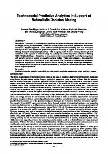
Fig. 1. Experiments with Delaunay graphs of sizes ranging from 50 to 1000 nodes: The upper diagrams show the mean separator size (left) and mean balance (right) with LT, Dj, and FCS. The lower diagrams show for FCS the ranges of the mean separator size (left) and mean balance (right), comparing BFS root and non-tree edge selection.
the first phase with a smallest valid BFS level, while Dj applies for around 15% of the BFS roots the last phase of the algorithm. Figure 1 shows clearly that FCS computes on average the best separators, while Dj is slightly better than LT. Considering the LEDA random graphs, both LT and Dj always have to pass the third phase. The mean separator size of FCS is only slightly better than that of Dj, while LT is by far worse. The mean balance with LEDA graphs is similar for all algorithms between 0.8 and 0.9. The lower diagrams in Figure 1 show the influence of BFS root selection and non-tree edge selection on separator size and balance. For FCS applied to the Delaunay graphs, the range of the mean of both the separator size and balance values are depicted, either over all possible BFS root nodes or over all possible non-tree edges. For example, the range of the mean separator size over all possible BFS root nodes is defined as follows: For every BFS root, determine the mean separator size over all possible non-tree edges. Then, the wanted range of the mean is the difference between the maximum and the minimum of these separator sizes among all BFS root nodes. The diagrams show that selection of the BFS root node is more decisive for the separator size than non-tree edge selection. Concerning balance, both selections are of similar importance.
graph
nodes edges diameter orig triang grid 10000 19800 198 67 20 rectangular 10000 19480 518 sixgrid 9994 14733 513 22 triangular 5050 14850 99 45 globe 10002 20100 101 101 t-sphere 10242 30720 96 96 diameter 10000 29994 3333 3333 del 10000 25000 56 45 10000 29971 52 48 del-max leda 9989 25000 18 15 leda-max 10000 29975 15 14 c-grid 10087 19904 212 72 c-globe 10090 20325 144 142 10005 29972 65 58 c-del-max c-leda-max 10005 29984 20 16 airfoil1 4253 12289 65 31 city2 2948 3564 131 14 city3 15868 16690 658 13
radius orig triang 100 50 260 10 257 11 66 34 76 67 80 80 1667 1667 46 36 43 39 11 8 9 8 106 36 73 71 34 29 11 8 36 21 66 9 329 9
LT min mean 82 106 20 27 21 28 58 83 100 119 160 169 3 4 206 300 204 314 76 216 56 205 38 78 4 96 74 318 78 209 50 89 15 39 28 53
Dj min mean 82 106 20 27 21 28 58 83 100 119 160 169 3 4 82 113 86 117 7 31 7 26 38 78 4 96 19 65 7 32 26 85 15 39 28 53
FCS min mean 89 99 20 20 21 21 58 68 100 106 160 164 3 3.3 65 75 74 79 5 8 6 10 5 6.4 4 12 5 8.3 4 4.5 26 35 4 9.5 4 6.8
Table 1. Large graphs:The table depicts the number of nodes and edges, the diameter and the radius for both the graph itself (orig) and a triangulation of it (triang) as well as for each of the algorithms LT, Dj, and FCS, all of them optimized on separator size with postprocessing applied, the minimum and mean separator sizes over all BFS root nodes; bold-face and italic figures indicate the best result(s) for the respective graph.
4.2
Large Graphs
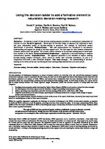
The second series of graphs that we experimented with, the large graphs, consists of 16 graphs of the categories mentioned in Section 3 of size roughly 10000 nodes (see Table 1). The rectangular graph represents a 20 × 500 raster, the sixgrid graph consists of 20 × 237 hexagons, the globe has 100 meridians and circles of latitude, and the t-sphere is constructed by 5 iterations. For c-grid, c-del-max and c-leda-max, the two copies of the respective graph are connected by 5 nodes, while for c-globe only 4 nodes are used to connect the two graphs. Main results. We investigated the performance in terms of separator size of LT, both unoptimized and optimized on separator size, Dj, and FCS, the latter ones optimized on separator size. We ran each of these algorithms for each graph while once making each node the root of the BFS tree. The results of the experiments regarding the separator sizes achieved by the various algorithms are listed in Table 1, and illustrated in Figure 2 by means of box plots that represent the middle fifty per cent of the data series (note that the whiskers here span the whole range of outcomes). The data shows that—except for the grid graphs—the smallest minimum separator is found by FCS, and concerning the mean separator size FCS achieves the best result
4
city3
city2
airfoil1
c-leda-max
c-del-max
c-globe
c-grid
leda-max
leda
del-max
del
diameter
t-sphere
globe
triang
6grid
rect
grid
0
1
2
3
Lipton&Tarjan (LT) Lipton&Tarjan (LT) optimized Djidjev (Dj) Fundamental Cycle Sep (FCS)
√ Fig. 2. Box plots depicting the separator sizes relative to n obtained with unoptimized LT (light-gray) and LT (gray), Dj (dark-gray), and FCS (black), the latter three optimized on separator size. The dashed lines indicate the range of all separators without postprocessing applied.
for all graphs under consideration. This, together with the fact that the boxes are clearly slender, and—except for c-globe—the ranges are minimal for FCS, suggests that FCS significantly outperforms the other algorithms in terms of separator size. In particular, this behavior is surprising for graphs with rather big diameter d and radius r (e.g., c-globe, globe, and diameter), since the guaranteed bound on the separator size is 2d + 1 (2r + 1, respectively; cf. the description of FCS on page 4) for FCS. For regular-structured graphs (i.e., grid-like, sphere approximation, and the diameter graphs) the separator sizes are similar and quite high for the three algorithms. For irregular graphs (i.e., leda, the graphs with small separator, and the real-world graphs), the picture looks different: The Dj algorithm always yields better results than the LT algorithm, and FCS is clearly superior to both Dj and LT. Furthermore, the minimum and mean separator sizes computed by FCS are by far below the guaranteed upper bounds. The running time considering one BFS root node is linear for all of our algorithms. However, for the algorithms LT and Dj, the constant crucially depends on the phase in which the algorithms terminate (cf., Section 2.2). The first two phases consist basically of a breadth-first search, while the computation of the
1.2
2.5
METIS FCS
city2
city3
airfoil1
c-del-max
c-leda-max
c-grid
c-globe
leda
leda-max
del
del-max
diameter
globe
t-sphere
triang
rect
6grid
grid
0.2 0.0
city2
city3
airfoil1
c-del-max
c-leda-max
c-grid
c-globe
leda
leda-max
del
del-max
diameter
globe
t-sphere
triang
rect
6grid
grid
0.0
0.5
0.4
1.0
0.6
1.5
0.8
2.0
1.0
METIS FCS
√ Fig. 3. Minimum separator sizes relative to n (left) and balance (right) computed with MeTiS (light-gray) and with FCS (black) optimized on separator ratio.
fundamental cycle requires expensive operations like embedding, triangulation, and copying. FCS, of course, computes a fundamental cycle and always needs the expensive operations. LT and Dj terminate after phase 1 with all grid-like graphs, sphere-approximating graphs, and with the diameter, c-grid, c-globe, and city graphs. In contrast, the LEDA, c-del-max, and c-leda-max graphs in the majority of cases require phase 3. For the Delaunay graphs, LT mostly terminates after phase 1, but Dj needs phase 3. The mean running time for LT (applying only phase 1) in the city3 graph, for example, is 0.04 seconds, while FCS involving a fundamental-cycle computation needs 0.71 seconds. Postprocessing. The subsequent experiments deal with the effect of postprocessing on the various algorithms. We found in a pre-study that the optimization of separator size and separator ratio should be accompanied by a combination of Dulmage-Mendelsohn optimization followed by node expulsion. Our results applying these combinations of postprocessing techniques can be summarized as follows (data not shown): On the one hand, for the grid-like and sphere-approximating graphs as well as the diameter graph, the separators found by the algorithms without postprocessing cannot be much improved. (Often the separators are already close to optimal solutions for these graphs.) On the other hand, for the remaining graphs, the separators computed by the algorithms Dj and LT are very large compared to an optimal solution, and in these cases the postprocessing greatly improves the separators. The separators computed by FCS can generally be improved only a little. Benchmark. To get an idea of the quality of the separators found by the algorithms, we compare them against separators obtained with the help of MeTiS [14], a graph partitioning tool collection. We applied MeTiS to partition the nodes into two sets and observed very high balances (meeting the requirement that each part encompass at least one third of the graph’s nodes) with quite few cut edges. From a partitioning thus obtained we computed a node separator by choosing an appropriate subset of the end-nodes of the edges forming the cut.
Separators determined by MeTiS are a trade-off between separator size and balance, so for the sake of a meaningful comparison, we contrast the MeTiS results and our algorithms optimized on separator ratio. Since among LT, Dj, and FCS optimized on separator ratio, the solutions computed by FCS were the best with respect to both separator size and balance, we compare MeTiS with FCS only. Figure 3 shows the best separator size and balance values. One may state that with FCS, the separator size is always at least as good as with MeTiS and balance is almost always comparable. Those graphs whose balance is considerably worse with FCS than with MeTiS (leda and city2) exhibit by far smaller separators with FCS, which suggests that the weighting between the two criteria, separator size and balance, seems to be more in favor of separator size with FCS, while MeTiS tends to prefer balance. Indeed, almost perfect balance can always be achieved with FCS optimized only on balance. 4.3
City Graphs
We consider a series of city graphs with numbers of nodes up to about 45,000. For these graphs we computed separations by the following linear-time procedure: run FCS on ten BFS trees of a given graph, determined by a random node as root, and from among these separations take the one with best separator ratio. The results of the experiments with the graph nodes edges size balance city graph series are depicted in the table city1 1429 3034 5 0.871 aside. Obviously, all city graphs have excity2 2948 3564 8 0.996 tremely small separators, which are also found city3 15868 16690 7 0.869 by our algorithm. The separators for the city4 20036 41476 10 0.789 city2 and city3 graphs, which had already city5 24106 53826 5 0.740 been included in the experiments of the precity6 38823 79988 8 0.704 vious section, are somewhat bigger than those city7 44878 90930 7 0.547 of the preceding experiment (8 and 7 instead of 4, resp.; see Table 1). This is due to the fact that: (i) the separator ratio is now optimized instead of the separator size; and (ii) we do not longer take into account every node as a BFS root.
5
Conclusions and Outlook
Our experiments have shown that, especially for graphs with small separators, there is a high potential for optimizing the separators computed by the algorithms. Both the postprocessing and in particular the Fundamental-Cycle Separation yielded almost-optimal separators with respect to separator size and balance. Applied to graphs whose triangulations have small diameter (which is true for many graphs, especially from real world), FCS is empirically and theoret√ ically superior to the classical algorithms guaranteeing separators of size O( n). Selection of the non-tree edge in the fundamental-cycle computation has a considerable influence on both criteria, and we are able to select the best during the respective algorithm. The choice of the BFS root also exhibits a great impact on
separator quality, mainly on its size. The experiments on city graphs confirmed that FCS, applied to a small random sample of BFS root nodes and separator ratio as optimization criterion yields excellent separators in linear time. An issue for further investigation would be to explore whether more sophisticated strategies for selecting an appropriate BFS root can be developed. In addition, we would like to investigate other parts of the algorithms that are also subject to arbitrary choices, namely triangulation and breadth-first search.
Acknowledgments The authors would like to thank Imen Borgi and J¨ urgen Graf for their assistance with parts of the implementation work and the anonymous referees for their detailed comments and very helpful hints for further research.
References 1. Lipton, R.J., Tarjan, R.E.: A separator theorem for planar graphs. SIAM Journal on Applied Mathematics 36 (1979) 177–189 2. Djidjev, H.N.: On the problem of partitioning planar graphs. SIAM Journal on Algebraic and Discrete Methods 3 (1982) 229–240 3. Djidjev, H.N., Venkatesan, S.M.: Reduced constants for simple cycle graph separation. Acta Informatica 34 (1997) 231–243 4. Aleksandrov, L., Djidjev, H.N., Guo, H., Maheshwari, A.: Partitioning planar graphs with costs and weights. In: ALENEX 2002. Volume 2409 of LNCS., Springer (2002) 98–110 5. Leighton, T., Rao, S.: Multicommodity max-flow min-cut theorems and their use in designing approximation algorithms. Journal of the ACM 46 (1999) 787–832 6. Mehlhorn, K.: Data Structures and Algorithms 1, 2, and 3. Springer (1984) 7. Kozen, D.: The Design and Analysis of Algorithms. Springer (1992) 8. Ashcraft, C., Liu, J.W.H.: Applications of the Dulmage-Mendelsohn decomposition and network flow to graph bisection improvement. Technical Report CS-96-05, Dept. of Computer Science, York University, North York, Ontario, Canada (1996) http://www.cs.yorku.ca/techreports/1996/CS-96-05.html. 9. Bourke, P.: Sphere generation (1992) http://astronomy.swin.edu.au/~pbourke/modelling/sphere/. 10. N¨ aher, S., Mehlhorn, K.: The LEDA Platform of Combinatorial and Geometric Computing. Cambridge University Press (1999) http://www.algorithmic-solutions.com. 11. Diekmann, R.: (Graph Partitioning Graph Collection) http://wwwcs.upb.de/fachbereich/AG/monien/RESEARCH/PART/graphs.html. 12. BARD: (Bay Area Regional Database) http://bard.wr.usgs.gov. 13. ESRI: (Environmental Systems Research Institute) http://www.esri.com. 14. Karypis, G.: (MeTiS) http://www-users.cs.umn.edu/~karypis/metis.