Enhancing Computational Thinking with

International Journal of Computer Applications (0975 – 8887) Volume 55– No.14, October 2012

Enhancing Computational Thinking with Spreadsheet and Fractal Geometry: Part 4 Plant Growth modeling and Space Filling Curves K.P Soman, Manu Unni V.G, Praveen Krishnan, V. Sowmya Centre for excellence in Computational Engineering and Networking (CEN), Amrita Vishwa Vidyapeetham, Coimbatore, Tamil Nadu, India

ABSTRACT String rewriting systems are another iterative process for creating fractals. The additional grammar formalism in L-systems allows us to build a richer variety of shapes. L-Systems are an efficient way to encode complicated images. With L-Systems different replacements can be made in different parts of the picture. LSystems can be extended to three dimensions, and have been used to make realistic forgeries of plants. They provide a good laboratory for learning about recursive processes, and pattern recognition. In this last article in the series, we explain L-System formalism initially developed for modeling plant growth. The concept can be also used for creating Space filling curves. The drawing of these plots in spreadsheet is explained. It is the first attempt in drawing all fractals in spreadsheet.

Keywords— Computational thinking, L-Systems, Space filling curves

1. INTRODUCTION The beauty of plants has attracted the attention of mathematicians for centuries. The Bilateral symmetry of leaves, the rotational symmetry of flowers, and the helical arrangements of scales in pine cones have been studied most extensively. The first is the elegance and relative simplicity of developmental algorithms, that is, the rules which describe plant development in time. The developmental processes are captured using the formalism of Lsystems [8]. They were introduced in 1968 by Lindenmayer as a theoretical framework for studying the development of simple multi-cellular organisms, and subsequently applied to investigate higher plants and plant organs. After the incorporation of geometric features, plant models expressed using L-systems became detailed enough to allow the use of computer graphics for realistic visualization of plant structures and developmental processes. The central concept of L-systems is that of rewriting. In general, rewriting is a technique for defining complex objects by successively replacing parts of a simple initial object using a set of rewriting rules or productions. The classic example of a graphical object defined in terms of rewriting rules is the snowflake curve (Figure 1.), proposed in 1905 by Koch von Koch . This construction is described in next section:

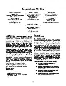
2. KOCH CURVES One begins with two shapes, an initiator and a generator. The generator is an oriented broken line made up of N equal sides of length r. Thus each stage of the construction begins with a broken line and consists in replacing each straight interval with a copy of the generator, reduced and displaced so as to have the same end points as those of the interval being replaced. Fig. 1(a-f) shows this process.

Fig. 1 Generation of Koch curve by repeated segment replacement: (a) Initiator, (b) generator, (c) After 1 iteration, i.e.; n=1, (d) n=2, (e) n=3, (f) n=4 While the Koch construction recursively replaces open polygons, rewriting systems that operate on other objects have also been investigated. The most extensively studied and the best understood rewriting systems operate on character strings. To give an example, the single rule: a → b a b transforms the string: a b a c into b a b b b a b c Prusinkiewicz in 1970s gave geometrical interpretation to the generated letters based on a LOGO-style turtle (A computer based graph drawing system in which the cursor is called a turtle and instruction to move the turtle in different direction is given by a set of different keys on keyboard) and presented several examples of fractals and plant-like structures using L-systems. The basic idea of turtle interpretation is given below. A state of the turtle is defined as a triplet (x, y, α), where the Cartesian

24

International Journal of Computer Applications (0975 – 8887) Volume 55– No.14, October 2012 coordinates (x, y) represent the turtle’s position, and the angle α, called the heading, is interpreted as the direction in which the turtle is facing. Given the step size d and the angle increment δ, the turtle can respond to commands represented by the following symbols F : Move forward a step of length d. The state of the turtle changes to (x’, y’,α), where x’ = x + d cos α and y’ = y + d sin α. A line segment between points (x, y) and (x’, y’) is drawn. f : Move forward a step of length d without drawing a line. + :Turn left by angle δ. The next state of the turtle is (x, y, α+δ). The positive orientation of angles is counterclockwise. −: Turn right by angle δ. The next state of the turtle is (x, y, α − δ). Given a string ν = FFF-FF-F-F+F+FF-F-FFF, the initial state of the turtle (x0, y0, α0=90) and fixed Interpretation parameters d (=1 unit) and δ(=90degree), the turtle interpretation of ν is shown in Fig. 2 (set of lines), drawn by the turtle in response to the string ν . Fig. 3 Quadratic Koch Island by L-System: (a) n=0, (b) n=1, (c) n=2, (d) n=3 Example 1: Let us draw the figure corresponding to the string FFF-FF-F-F+F+FF-F-FFF Where starting angle of the turtle position is assumed to be 90, + is 90 degree Anti-clockwise rotation and ‘–‘ for 90 degree clockwise rotation. The figure must look as shown in Fig. 4.

Fig. 2 Drawing a figure by string interpretation Specifically, this method can be applied to interpret strings which are generated by L-systems. For example, Fig. 3(a-d) presents four approximations of the quadratic Koch island. Fig. 3 is obtained by interpreting strings generated by the following L-system: Initiator ω : F − F − F − F Generator p : F → F − F + F + FF − F − F + F The images correspond to the strings obtained in derivations of length 0 to 3. The angle increment δ is equal to 900. The step length d is decreased four times between subsequent images, making the distance between the endpoints of the successor polygon equal to the length of the predecessor segment. This step length reduction is usually given as a parameter.

2.1 Implementation in excel Now we see how we implement string interpretation based drawing in Spreadsheet.

Fig. 4 Plot for “FFF-FF-F-F+F+FF-F-FFF” To implement this we use two important functions (formula) available in Excel. First one is the MID Function. This is used to parse the whole string into a column of letters such that a cell contains only one letter. Once parsed, corresponding coordinates based on previous coordinates and the value of angle can be obtained. We use one separate column for tracking the angle corresponding to each alphabet. The syntax for the MID function is:= MID ( Text , Start_num , Num_chars ) Text - the piece of string we want to parse. Start_num - specifies the starting character from the left of the data to be kept. Num_chars - specifies the number of characters to the right of the Start_num to be retained. The output should look like column B as shown in Fig. 5 starting from B3. By writing a formula in B3 and by copying down we should be able to get parsed characters. This is achieved using the formula =MID($B$2,ROW(A1),1)

25

International Journal of Computer Applications (0975 – 8887) Volume 55– No.14, October 2012 We expand this to three levels as shown in Fig. 6. Only part of the string is shown in Figure. Then write a formula in K4 and pull (copy) down to K6. The formula in K4 is =SUBSTITUTE(K3,"F",$K$2) . This substitutes each letter F in K3 by the string in K2 which produces a long string in K4. The final string is in K6. We sparse this column wise as done earlier. This we do in Columns B to E.

Fig. 5 Snapshot of Excel sheet that generates coordinates of the vertices generated by LOGO-interpretation of “FFF-FFF-F+F+FF-F-FFF” It uses a function Row( ). It returns row number of the argument cell. Here the argument of the function is A1. It is known that row of A1 is 1. When it is pull down (copy down) the formula one cell down, automatically the argument changes to A2 and hence it returns 2. Thus it is indeed a powerful function. Following are the further steps required:  



In cell C2 we write 90 as starting angle value In Cell D2 and E2 write 0 as starting coordinates respectively of x and y Angle update - In cell E3 we update angle value. The angle is updated if and only if a + or – is encountered in the parsed string. If a + is encountered add 90 and if a – is encountered add -90 otherwise previous angle is retained. While updating angle may exceed 360 degree. The Mod function is used to bring it down between 0 and 360. The following formula achieves this. =IF(B3="+",MOD(C2+90,360),IF(B3="-",MOD(C290,360),C2)) Coordinate update - In cell D3 the updating formula for xcoordinate is updated as follows =IF(B3="F", D2+COS(RADIANS(C3)),D2) In cell E3 the updating formula for y-coordinate is updated as follows =IF(B3="F", E2+SIN(RADIANS(C3)),E2) Now by copying the formula down from B3:E3 to 21(number of characters in the string) cells, and plotting an x-y scatter chart for the data in columns D and E the required Figure is obtained.

Fig. 7 Snapshot of Excel sheet that generates coordinates of the vertices generated by LOGO-interpretation of Level-3 string in Fig. 6 The formula in B3 is =MID($K$6,ROW(A1),1) . This formula is pull down to parse the string. The output figure after formatting is as shown in Fig. 8.

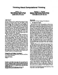
3. SPACE FILLING HILBERT CURVE Around 1890, an Italian mathematician Giuseppe Peano (1858 1932) surprised the mathematical world by discovering what was called "space-filling curve". His curve was constructed in such a way that there was no point on the plane that its twisted curve would not include. It means that a line, which is considered as one dimensional object, has one to one mapping to all the points on the plane, which are two dimensional (See Fig. 9).

Fig. 8 Line plot of the Generator: FF-F-F-F-FF with initiator F-F-F-F for the string at level-3 in spreadsheet.

Next lets see how to use string rewriting to generate complicated figures. Let the generator and initiator string be as follows. Generator: FF-F-F-F-FF. We enter this in cell K1 Initiator: F-F-F-F. We enter this in cell K2

Fig. 6 Snapshot of Excel sheet that generates strings by repeated substitution

Fig. 9 (a) Giuseppe Peano, (b) Three iterations of Peano Space filling curves

26

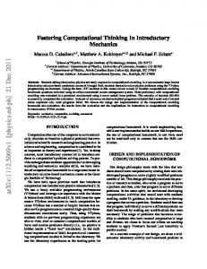
International Journal of Computer Applications (0975 – 8887) Volume 55– No.14, October 2012 It was followed by another by D Hilbert (See Fig. 10).

3.1 Implementation in Excel The Spread sheet implementation of Hilbert curve using two generators (See Fig. 11) is discussed in this section. Note that only the implementation is discussed and not how the generators are obtained. The two generators are denoted as L and R generators. The corresponding strings are given in cell H2 and H3. The initiator string is given in H4. One has to perform 5 levels of rewriting. Note that letter F has no rewrite string. However whenever an F is encountered the turtle has to move forward by one unit. Another important point to be noted is that in level (stage) of substitution, one has to perform two substitutions to a given string. This causes a problem. Suppose string abc is to be replaced with the rules a -> bc and b> ca. The required out is bccac which is obtained by parallel substitution. But the output will be different for sequential substitution. To overcome this problem, we introduce a dummy variable before substitution. So in H5 we write the formula as =SUBSTITUTE(SUBSTITUTE(SUBSTITUTE(H4,"L","C"),"R" ,$H$3),"C",$H$2) Here before the two required substitution, a new substitution (the innermost) is introduced where L is replaced by C, Then R is replaced by its substitution string, followed by a substitution of letter C by the substitution-string corresponding to letter L. The remaining part of the steps is same as the one done for other experiments. The output is as shown in Fig. 12.

Fig. 12 Hilbert Curve in spreadsheet [ : Push the current state of the turtle onto a pushdown stack. The information saved on the stack contains the turtle’s position and orientation, and possibly other attributes such as the color and width of lines being drawn.] : Pop a state from the stack and make it the current state of the turtle. No line is drawn, although in general the position of the turtle changes. Example 1. Design an L-system, which will generate a simple branched structure: Following are the Axiom (initiator) and Rules (also known as productions rules) for rewriting

Fig. 13 Rule interpretation of Bracketed L-System

Fig. 10 (a) D Hilbert, (b) Four iterations of Hilbert Space filling curves

With a use of the rule we obtain an order of strings: 0. step: F 1. step: F[+F][-F] 2. step: F[+F][-F][+F[+F][-F]][-F[+F][-F]] Etc. The L-system after 6 steps looks like bush shown in Fig. 14. Note that step length is constant for every iteration. Example 2.During the growth of the tree certain part of the tree should remain in same length and other part to grow. This can be modeled by two rules as given below. Axiom: X p1: X → F-[+X]+F[-X]+X p2: F → FF

Fig. 11 Snapshot of Excel sheet that do 5 levels of expansion for drawing Hilbert curve

If we assume step length d is replaced by d/2 after each iteration, then the rule F → FF ensures that the F part of the tree in any iteration remain there in the subsequent stages without any further growth. Representation of a plant after 5 steps of derivation is shown in Fig. 15. A model of plant is more realistic than on the figure. The turning angle is 22.5°. This kind of branching is characteristic for apple tree.

4. BRANCHING STRUCTURES AND BRACKETED L-SYSTEMS Plant kingdom is dominated by branching structures. For this, an extension of turtle interpretation to strings with brackets was introduced. They are interpreted by the turtle as follows:

27

International Journal of Computer Applications (0975 – 8887) Volume 55– No.14, October 2012 EXAMPLE 3. Axiom X P1 : X → F[+X][-X]FX P2 : F → FF divisor = 2.0 angle = 27.9 After 9 iterations the figure is as shown in Figure 16. Figure 17(a-e) are the some of the trees and their respective axiom and rules. L-system concept can be easily extended to 3D (See Fig. 18). Readers may refer references [1-9] for more details. Fig. 14 A tree whose trunk length remain same

Fig. 15 An L-system tree drawn using programming

Fig. 18 A 3D L-system tree Note that all the tree plots are drawn using programming. Of course it can be implemented in spreadsheet without programming. However it requires a method to implement stack operation. It is left an exercise to the reader.

5. SUMMARY

Fig. 16 L-system trees with different generators

An L-system is a substitution system in which rules are used to operate on a string consisting of letters of a certain alphabet. String rewriting systems are also variously known as rewriting systems, reduction systems, or term rewriting systems. String rewriting is a particularly useful technique for generating successive iterations of certain types of fractals, such as the tress and space filling curves. Spreadsheet can be used to generate such fractals without programming and hence can be introduced at high school for experimentation.

6. REFERENCES [1] Barnsley,M., F., “Fractals Everywher”e, 1993 [2] Peters, E., E., “Chaos and Order in the Capital Markets: A New View of Cycles, Prices, and Market Volatility”, Wiley, 2nd Edition, 1996 [3] Devaney, R., Keen, L., eds., “Chaos and Fractals: The Mathematics behind the Computer Graphics”, American Mathematical Society, Providence, RI, 1989 Fig. 17 L-System Tree

[4] Falconer, K., “Fractal Geometry: Mathematical Foundations and Applications”, Wiley, (2003)

28

International Journal of Computer Applications (0975 – 8887) Volume 55– No.14, October 2012 [5] Peitgen, H., Juergens, H., Saupe, D., “Fractals for the Classroom. Springer”, (1991)

[8] Przemyslaw.P, Lindenmayer,A., “Algorithmic beauty of Plants”, Springer Verelag, 1990

[6] Mandelbrot, B., “The Fractal Geometry of Nature”, published by W. H. Freeman, 1983

[9] Flake, G.W, “Computational Beauty of Nature”, MIT press, 1998

[7] Mumford, D., Caroline Series, Wright, D., “Indra's Pearls: The Vision of Felix Klein”, Cambridge University Press, 2002

29