Enhancing Performance of Cloud Computing ...

Enhancing Performance of Cloud Computing Services Through Improving Reliability and Taming Latency

by Yu Xiang

A Dissertation Submitted to The Faculty of The School of Engineering and Applied Science of The George Washington University in partial fulfillment of the requirements for the degree of Doctor of Philosophy

August 31, 2015

Dissertation directed by Tian Lan Assistant Professor of Engineering and Applied Science

The School of Engineering and Applied Science of The George Washington University certifies that Yu Xiang has passed the Final Examination for the degree of Doctor of Philosophy as of July 10, 2015 . This is the final and approved form of the dissertation.

Enhancing Performance of Cloud Computing Services Through Improving Reliability and Taming Latency

Yu Xiang

Dissertation Research Committee:

Tian Lan, Assistant Professor of Engineering and Applied Science, Dissertation Director Howie Huang, Associate Professor of Engineering and Applied Science, Committee Member Suresh Subramaniam, Professor of Engineering and Applied Science, Committee Member

ii

Abstract

Enhancing Performance of Cloud Computing Services Through Improving Reliability and Taming Latency

Thesis Statement: With the growing usage of cloud services in a number of fields, more and more research work is focusing on improving the overall performance of the cloud. As data centers in the cloud are coordinating hundreds of thousands of heterogeneous tasks everyday, meeting everyones requirements in various aspects becomes a very complicated problem. In this work we (i) provide a quantitative framework to model key performance metrics such as latency and reliability in cloud computing, and (ii) develop a cloud resource management system that dynamically optimize resource allocation to deliver differentiated cloud services satisfying heterogeneous requirements. The growth of cloud computing services is far outstripping the overall expansion of IT, as anticipated, the worldwide cloud computing market will grow at a 36% compound annual growth rate through 2016, and this explains why people become more and more concerned about the quality of cloud service. Cloud computing in Modern data centers deliver resources over the cloud for clients to run various applications and jobs with diverse requirements, such as availability and security, performance level, resource utilization, etc. In this project we focus on the performance of reliability level and service latency, as these two aspects are key factors reflecting the security and performance level of cloud services. Cloud applications may have various requirements on reliability and service latency, although offering equal reliability and service latency level to all users benefits everyone at the same time, users may find such an approach either too inadequate or too expensive to fit their individual requirements, which may vary dramatically. Our goal in this work is to provide reliability as an elastic service and optimize joint service latency to cloud customers. In the aspect of

reliability, we first propose a novel method for providing reliability as an elastic and on-demand service, which allows user reliability levels to be jointly optimized based on an assessment of their individual requirements and total available resources in the data center. Further inspired by the CSMA protocol in wireless congestion control, we improved the framework for contention-free checkpoint scheduling. In the aspect of service latency, we optimize latency and cost in the mean time while increasing reliability levels by applying proper erasure code in distributed storage systems, we provide an insightful upper bound on the average service delay of such erasure-coded storage with arbitrary service time distribution and consisting of multiple heterogeneous files. Then the system model is further extended to a data center storage system with a hierarchical structure, considering the impact of network bandwidth bottleneck on service latency. We also extended the system model to provide differentiated services among different tenants and tries to minimize the average latency of files in the system. For scheduling tenant requests at different servers, we investigate two different queuing techniques to achieve differentiated services. All three system models have been validated by experimental results and show significant latency reduction.

iv

Table of Contents

Abstract

iii

Table of Contents

v

List of Figures

vi

List of Tables

xi

1 Introduction

1

1.1

Cloud Computing Services . . . . . . . . . . . . . . . . . . . . . . . .

1

1.2

Reliability in Cloud Computing . . . . . . . . . . . . . . . . . . . . .

2

1.3

Latency Performance in Cloud Storage . . . . . . . . . . . . . . . . .

3

1.4

Related Work . . . . . . . . . . . . . . . . . . . . . . . . . . . . . . .

6

1.5

Overview . . . . . . . . . . . . . . . . . . . . . . . . . . . . . . . . . .

8

2 Improving Cloud Performance in Reliability 2.1

2.2

2.3

Providing Reliability as an Elastic Service . . . . . . . . . . . . . . .

10

2.1.1

Peer-to-Peer Checkpointing and ReliabilityAnalysis . . . . . .

11

2.1.2

Reliability Optimization . . . . . . . . . . . . . . . . . . . . .

16

2.1.3

Simulations and Numerical Results . . . . . . . . . . . . . . .

19

Optimizing Reliability Through Contention-Free, Distributed Checkpoint Scheduling . . . . . . . . . . . . . . . . . . . . . . . . . . . . .

22

2.2.1

Need for Contention-Free Checkpoint Scheduling . . . . . . . .

23

2.2.2

CSMA-Based Checkpointing Scheduling . . . . . . . . . . . .

24

2.2.3

Reliability Analysis and Optimization . . . . . . . . . . . . . .

25

2.2.4

Implementation and Evaluation . . . . . . . . . . . . . . . . .

32

Summary . . . . . . . . . . . . . . . . . . . . . . . . . . . . . . . . .

37

3 Improving Cloud Performance in Service Latency 3.1

10

Joint Latency and Cost Optimization for Erasure-coded Cloud Storage v

38 38

3.2

3.3

3.4

3.5

3.6

3.1.1

System Model and Probabilistic Scheduling

. . . . . . . . . .

42

3.1.2

Latency Analysis and Upper Bound . . . . . . . . . . . . . . .

47

Joint Latency-Cost Optimization . . . . . . . . . . . . . . . . . . . .

50

3.2.1

Problem Formulation . . . . . . . . . . . . . . . . . . . . . . .

50

3.2.2

Constructing Convex Approximations . . . . . . . . . . . . . .

51

3.2.3

Algorithm JLCM and Convergence Analysis . . . . . . . . . .

54

Implementation and Evaluation . . . . . . . . . . . . . . . . . . . . .

56

3.3.1

Tahoe Test-bed . . . . . . . . . . . . . . . . . . . . . . . . . .

56

3.3.2

Implementation and Evaluation . . . . . . . . . . . . . . . . .

58

Latency Optimization in Data Center Networking with Erasure Coded Files . . . . . . . . . . . . . . . . . . . . . . . . . . . . . . . . . . . .

67

3.4.1

System Model in Data Center Network . . . . . . . . . . . . .

68

3.4.2

Analyzing Service Latency for Data Requests . . . . . . . . .

69

3.4.3

Joint Latency Optimization . . . . . . . . . . . . . . . . . . .

71

3.4.4

Implementation and Evaluation . . . . . . . . . . . . . . . . .

75

Multi-Tenant Latency Optimization in Erasure-Coded Storage with Differentiated Services . . . . . . . . . . . . . . . . . . . . . . . . . .

82

3.5.1

System Model with Differentiated Services . . . . . . . . . . .

83

3.5.2

Differentiated Latency Analysis . . . . . . . . . . . . . . . . .

85

3.5.3

Joint Latency Optimization with Differentiated Services

. . .

88

3.5.4

Latency Optimization for Weighted Queues . . . . . . . . . .

92

3.5.5

Implementation and Evaluation . . . . . . . . . . . . . . . . .

95

3.5.6

Experiments and Evaluation . . . . . . . . . . . . . . . . . . .

95

Summary . . . . . . . . . . . . . . . . . . . . . . . . . . . . . . . . . 101

4 Conclusion and Future Work

103

4.1

Conclusion . . . . . . . . . . . . . . . . . . . . . . . . . . . . . . . . . 103

4.2

Future Work . . . . . . . . . . . . . . . . . . . . . . . . . . . . . . . . 104

vi

List of Figures

1.1

An erasure-coded storage of 2 files, which partitioned into 2 blocks and encoded using (4, 2) and 3, 2 MDS codes, respectively. Resulting file chunks are spread over 7 storage nodes. Any file request must be processed by 2 distinct nodes that have the desired chunks. Nodes 3, 4 are shared and can process request for both files. . . . . . . . . . . . . . . . . . . . . . .

2.1

Task checkpoint and recovery model. Checkpointing all VMs belonging to a task is synchronized..

2.2

5

. . . . . . . . . . . . . . . . . . . . . . . . . . .

13

Illustrations of peer-to-peer checkpointing with fat-tree topology, where traffics are distributed over the entire network and never reach top-level core switches. . . . . . . . . . . . . . . . . . . . . . . . . . . . . . . . . .

14

2.3

Algorithm for joint checkpoint scheduling and routing to maximize reliability. 20

2.4

Comparision of reliability on Fat-tree topology. Our proposed algorithm with peer-to-peer checkpointing shows significant reliability improvement.

2.5

21

Impact of changing link capacity. Our proposed algorithm with peer-topeer checkpointing outperforms the centralized scheme even if the bottleneck link capacity is increased to Cs = 40Gbps. . . . . . . . . . . . . . .

2.6

22

Fully coordinated pipeline checkpoint schedule significantly reduces contention and improves reliability over parallel checkpoint schedule. Reliability calculated with 8 failures/year. . . . . . . . . . . . . . . . . . . . .

2.7

24

Our contention-free, distributed checkpoint scheduling protocol inspired by CSMA. . . . . . . . . . . . . . . . . . . . . . . . . . . . . . . . . . . .

25

2.8

Example: 3 jobs and corresponding Markov Chain. . . . . . . . . . . . .

27

2.9

Comparison of the reliability values from our theoretical analysis with a prototype experiment using 24 VMs in Xen. Our reliability analysis can accurately estimate reliability in the proposed contention-free checkpoint scheduling protocol within a margin of ±1%.

vii

. . . . . . . . . . . . . . .

33

2.10 Plot convergence of sensing rates λ1 , λ2 when Hill Climbing local search [26] is employed to solve the reliability optimization in (2.31) with 2 classes of jobs and a utility 2R1 + R2 . The algorithm converges within only a few local updates to the optimal sensing rates. . . . . . . . . . . . . . . . . .

34

2.11 Reliability for different failure rates. . . . . . . . . . . . . . . . . . . . . . .

35

2.12 Reliability for different checkpoint time intervals. . . . . . . . . . . . . . . .

35

2.13 Reliability of 128 jobs for both contention-free and contention-oblivious checkpoint scheduling. . . . . . . . . . . . . . . . . . . . . . . . . . . . . . . . .

36

2.14 Normalized downtime for different annual failure rates. . . . . . . . . . . . .

36

2.15 Reliability for different VM sizes. . . . . . . . . . . . . . . . . . . . . . . .

37

3.1

An erasure-coded storage of 2 files, which partitioned into 2 blocks and encoded using (4, 2) and (3, 2) MDS codes, respectively. Resulting file chunks are spread over 5 storage nodes. Any file request must be processed by 2 distinct nodes that have the desired chunks. Nodes 3, 4 are shared and can process requests for both files. . . . . . . . . . . . . . . . . . . .

3.2

40

Functioning of (a) an optimal scheduling policy and (b) a probabilistic scheduling policy. . . . . . . . . . . . . . . . . . . . . . . . . . . . . . . .

43

3.3

Algorithm JLCM: Our proposed algorithm for solving Problem JLCM. .

51

3.4

Projected Gradient Descent Routine, used in each iteration of Algorithm JLCM. . . . . . . . . . . . . . . . . . . . . . . . . . . . . . . . . . . . . .

3.5

Our Tahoe testbed with average ping (RTT) and bandwidth measurements among three data centers in New Jersey, Texas, and California . . . . . .

3.6

52

56

Comparison of actual service time distribution and an exponential distribution with the same mean. It verifies that actual service time does not follow an exponential distribution, falsifying the assumption in previous work [70, 78]. . . . . . . . . . . . . . . . . . . . . . . . . . . . . . . . . .

viii

59

3.7

Comparison of our upper bound on latency with previous work [2] and [50]. Our bound significantly improves previous result under medium to high traffic and comes very close to that of [50] under low traffic (with less than 4% gap).

3.8

. . . . . . . . . . . . . . . . . . . . . . . . . . . . . . . .

60

Convergence of Algorithm JLCM for different problem size with r = 1000 files for our 12-node testbed. The algorithm efficiently computes a solution in less than 250 iterations. . . . . . . . . . . . . . . . . . . . . . . . . . .

3.9

61

Comparison of Implementation results of Algorithm JLCM with some oblivious approaches. Algorithm JLCM minimizes latency-plus-cost over 3 dimensions: load-balancing (LB), chunk placement (CP), and erasure code (EC), while any optimization over a subset of the dimensions is non-optimal. 62

3.10 Actual service latency distribution of an optimal solution from Algorithm JLCM for 1000 files of size 150M B using erasure code (12,6), (10,7), (10,6) and (8,4) for each quarter with aggregate request arrival rates are set to λi = 0.118 /sec . . . . . . . . . . . . . . . . . . . . . . . . . . . . . . . .

63

3.11 Evaluation of different chunk sizes. Latency increases super-linearly as file size grows due to queuing delay. Our analytical latency bound taking both network and queuing delay into account tightly follows actual service latency,with error percentage less than 9%. . . . . . . . . . . . . . . . . .

64

3.12 Evaluation of different request arrival rates. As arrival rates increase, latency increases and becomes more dominating in the latency-plus-cost objective than storage cost. The optimal solution from Algorithm JLCM allows higher storage cost, resulting in a nearly-linear growth of average latency. . . . . . . . . . . . . . . . . . . . . . . . . . . . . . . . . . . . .

65

3.13 Visualization of latency and cost tradeoff for varying θ = 0.5 second/dollar to θ = 200 second/dollar. As θ increases, higher weight is placed on the storage cost component of the latency-plus-cost objective, leading to less file chunks and higher latency.

. . . . . . . . . . . . . . . . . . . . . . .

3.14 Our Tahoe testbed with ten racks and each has 8 Tahoe storage servers

ix

. . .

66 76

3.15 Convergence of Algorithm JLWO with r=1000 requests for heterogeneous files from each rack on our 80-node testbed. Algorithm JLWO efficiently compute the solution in 172 iterations. . . . . . . . . . . . . . . . . . . . . . . . . .

77

3.16 Actual service time distribution of chunk retrieval through intra-rack and interrack traffic for weighted queuing; each of them has 1000 files of size 100M B using erasure code (7,4) with the aggregate request arrival rate set to λi = 0.25 /sec in each model . . . . . . . . . . . . . . . . . . . . . . . . . . . . . . .

78

3.17 Comparison of average latency with different access patterns. Experiment is set up for 100 heterogeneous files, each with 10 requests. The figure shows the percentage that these 1000 requests are concentrated on the same rack. Aggregate arrival rate 0.25/sec, file size 200M. Latency improved significantly with weighted queuing. Analytic bound for both cases tightly follows actual latency as well. . . . . . . . . . . . . . . . . . . . . . . . . . . . . . . . . .

79

3.18 Evaluation of different file sizes in the weighted queuing model. Aggregate rate 0.25/sec. Compared with Tahoe’s built-in upload/download algorithm, our algorithm provides relatively lower latency with heterogeneous file sizes. Latency increases as file size increases. Our analytic latency bound taking both network and queuing delay into account tightly follows actual service latency.

80

3.19 Evaluation of different request arrival rate in weighted queuing. File size 200M. Compared with Tahoe’s built-in upload/download algorithm, our algorithm provides relatively lower latency with heterogeneous request arrival rates. Latency increases as requests arrive more frequently. Our analytic latency bound taking both network and queuing delay into account tightly follows actual service latency for both classes. . . . . . . . . . . . . . . . . . . . . . . . . . . . .

81

3.20 System evolution for high/Low priority queuing . . . . . . . . . . . . . .

84

3.21 System evolution for weighted queuing . . . . . . . . . . . . . . . . . . .

85

3.22 Convergence of Algorithm Priority and Algorithm Weighted with r=1000 requests for heterogeneous files on our 12-node testbed. Both algorithms efficiently compute the solution in 175 iterations. . . . . . . . . . . . . . . . . .

x

96

3.23 r = 1000 file requests for different files of size 100M B, aggregate request arrival rate for both classes is 0.28/sec for both priority/weighted queuing; varying C2 to validate our algorithms, weighted queuing provides more fairness to class 2 requests. . . . . . . . . . . . . . . . . . . . . . . . . . . . . . . . . . . . .

98

3.24 Evaluation of different file sizes in priority queuing. Both experiment and bound statistics are using the secondary axis. Latency increases quickly as file size grows due to the queuing delay of both classes in priority queuing. Our analytic latency bound taking both network and queuing delay into account tightly follows actual service latency.

. . . . . . . . . . . . . . . . . . . . . . . . .

98

3.25 Evaluation of different request arrival rates in priority queuing. Fixed λ2 = 0.14/sec and varying λ1 . As arrival rates of high priority class increase, latency of low priority requests shows logarithm growth. . . . . . . . . . . . . . . . .

99

3.26 Evaluation of different file sizes in weighted queuing. Latency increase shows more fairness for class 2 requests. Our analytic latency bound taking both network and queuing delay into account tightly follows actual service latency for both classes. . . . . . . . . . . . . . . . . . . . . . . . . . . . . . . . .

100

3.27 Evaluation of different request arrival rates in weighted queuing. As the arrival rate increases, latency increase shows more fairness for class 2 requests compared to priority queuing.

. . . . . . . . . . . . . . . . . . . . . . . . . . . . . . 101

xi

List of Tables

2.1

Main notation. . . . . . . . . . . . . . . . . . . . . . . . . . . . . . . . .

12

3.1

Main notation. . . . . . . . . . . . . . . . . . . . . . . . . . . . . . . . .

41

xii

Chapter 1 Introduction 1.1

Cloud Computing Services

Cloud computing is the use of computing resources (hardware and software) that are delivered as a service over a network, its main target is to provide service with an array of on-demand computing infrastructures and services through the Internet. Thus cloud computing is promising to provide high-quality and low-cost services by payper-use model in which guarantees are offered by the cloud service providers through customized SLA (Service Level Agreement). Today many companies such as Google, Microsoft, Amazon EC2, etc., have launched cloud services and these cloud providers are all competing to satisfy their customers with high quality, efficient service with low cost in the mean time. Literature shows that to achieve this ambitious goal, cloud computing faces a number of challenges (i) flexibility, to deliver appropriate service level to private and business consumers with various service level requirements; (ii) scalability, to serve diverse customers (private user, corporate enterprise, etc.); (iii) reliability, to provide high level of service continuity and increase the ability to recover from failures and disasters. (iv) rapidity/high performance, to complete service with high quality within the time period cloud users expected. This project focus on two main challenges for cloud service providers, (a) providing flexible and contention-free reliability level for cloud customers and (b) latency optimization to improve over all latency performance for differentiated cloud customers. Next we will introduce the background on research work in these two aspects of cloud service respectively.

1

1.2

Reliability in Cloud Computing

In public clouds like the EC2 Cloud by Amazon Web Services, reliability is only provided as an inelastic and predetermined service parameter. For instance, the service-level agreement (SLA) of Amazon EC2 states that customers can expect an availability level of 99.95% [1], which corresponds to a four hour downtime per year. Although this level of availability may satisfy the average population, other customers who need higher levels of availability have to acquire in-house support to harden the operating system and the applications running within their virtual machine instances in order to enhance the reliability of crucial applications. Existing solutions for handling cloud reliability focus on two types of customers: those who care and those who do not. However, customers that want availability between 99.95% and 99.999% are forced to spend much effort (and money) to patch up what commodity clouds, such as EC2, can offer. This presents an opportunity for cloud providers to offer reliability as a service (RaaS), designed to protect the instances their customers spin up. Flexible SLAs for reliability can be introduced to define customer expectations and allow reliability-aware pricing mechanism. With the introduction of pay-per-use reliability services, cloud customers could choose reliability components they require on a feature-by-feature basis. Achieving a desired reliability level could be a single check box away. For cloud service providers, reliability as a service presents an additional source of revenue and value to their services. To be successful, reliability services need to be streamlined and automated as much as possible. The inherent fault tolerance of modular design in cloud computing empowers an effective defense against failures and disasters, and the resource sharing mechanism makes such defense not only superior but also low cost. Therefore, we believe an effective fault-tolerant strategy should exploit these advantages of the cloud computing environment to provide reliability as an elastic service to cloud customers. Specifically, in this project, when we try to improve the reliability level, we focus on the recovery aspect because it has a more direct impact on the system availability. Also as there are hundreds of thousands of heterogeneous jobs running 2

in a data-center, a physical server can be hosting a number of co-located jobs, where the techniques (checkpointing and data replication, etc.) that are taken to maintain a certain reliability level from different jobs may introduce severe contention on shared resources, so in this project we are improving joint reliability through a distributed and contention-free scheduling of VM (virtual machine) checkpointing to offer reliability as a transparent, elastic service in data-centers.

1.3

Latency Performance in Cloud Storage

Beyond than reliability, we also consider service latency as a performance metric, as users typically have various requirements of latency performance in cloud services [10], and for this aspect of service requirement, we consider erasure-coded distributed storage system as an application among cloud services particularly, not only because of its popularity, but also because that this kind of application has erasure code to ensure reliability level as well. Consumers are increasingly storing their documents and media in the cloud, businesses are relying on Big Data analysis and migrating their traditional IT infrastructure to the cloud. These trends cause the online data storage demand to rise faster than Moores Law. The increased storage demands have led companies to launch cloud storage services like Amazon’s S3 and personal cloud storage services like Apple’s iCloud, DropBox, Google Drive and Microsoft’s SkyDrive. Storing redundant information on distributed servers can increase reliability for storage systems, since users can retrieve duplicated pieces in case of disk, node, or site failures. As cloud storage is growing at an unprecedented speed, latency is playing a more and more important role in the expansion of online data storage. Studies done at Google and Amazon show that Web users are quite sensitive to latency: even a 100ms increase in latency causes measurable revenue losses. Research challenges arise in novel solutions to reduce the latency in cloud storage as much as possible. Erasure coding has been widely studied for distributed storage systems and used by companies like Facebook and Google since it provides space-optimal data redundancy to protect against data loss. There is, however, a critical factor that affects the 3

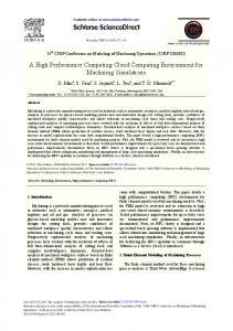
service quality that the user experiences, which is the delay in accessing the stored file. In distributed storage, the bandwidth between different nodes is frequently limited and so is the bandwidth from a user to different storage nodes, which can cause a significant delay in data access and perceived as poor quality of service. In this paper, we consider the problem of jointly minimizing both service delay and storage cost for the end users. While a latency-cost tradeoff is demonstrated for the special case of a single file, much less is known about the latency performance of multiple files that are coded with different parameters and share common storage servers. The main goal on the latency performance side of this project can be illustrated by an abstracted example shown in Fig. 3.1. We consider two files, each partitioned into k = 2 blocks of equal size and encoded using maximum distance separable (MDS) codes. Under an (n, k) MDS code, a file is encoded and stored in n storage nodes such that the chunks stored in any k of these n nodes suffice to recover the entire file. There is a centralized scheduler that buffers and schedules all incoming requests. For instance, a request to retrieve file A can be completed after it is successfully processed by 2 distinct nodes chosen from {1, 2, 3, 4} where desired chunks of A are available. Due to shared storage nodes and joint request scheduling, delay performances of the files are highly correlated and are collectively determined by control variables of both files over three dimensions: (i) the scheduling policy that decides what request in the buffer to process when a node becomes available, (ii) the placement of file chunks over distributed storage nodes, and (iii) erasure coding parameters that decides how many chunks are created. A joint optimization over these three dimensions is very challenging because the latency performance of different files are tightly entangled. While increasing erasure code length of file B allows it to be placed on more storage nodes, potentially leading to smaller latency (because of improved load-balancing) at the price of higher storage cost, it inevitably affects service latency of file A due to resulting contention and interference on more shared nodes. Later on we further extended the system model to a data center storage system with a hierarchical structure, considering the impact of network bandwidth bottleneck 4

5

3

1

4 File A

2

(4,2) coding 1: a1 2: a2 3: a1+a2 4: a1+2a2

File B

Scheduler

(3,2) coding 5: b1 6: b2 7: b1+b2

…… Requests

Figure 1.1: An erasure-coded storage of 2 files, which partitioned into 2 blocks and encoded using (4, 2) and 3, 2 MDS codes, respectively. Resulting file chunks are spread over 7 storage nodes. Any file request must be processed by 2 distinct nodes that have the desired chunks. Nodes 3, 4 are shared and can process request for both files.

on service latency, which is a major bottleneck for most data-center networks. In this model erasure coded files are stored on distributed racks and we assume that file access requests may be generated from anywhere inside the data center, e.g., a virtual machine spun up by a client on any of the racks. Due to limited bandwidth available at both top-of-rack and aggregation switches, a simple First Come First Serve (FCFS) policy to schedule all file requests indifferently falls short on minimizing service latency, not only because of its inability to differentiate heterogeneous flows or adapt to varying traffic patterns, but also due to the entanglement of different file requests. Without proper coordination in processing each batch of chunk requests that jointly reconstructs a file, service latency is dominated by staggering chunk requests with the worst access delay performance, significantly increasing overall latency in the data center. To avoid this, network bandwidth must be apportioned among different intra- and inter-rack data flows in line with their traffic statistics. The optimization goal is to minimize average joint latency for all requests in the system, the optimization has one more control knob: the bandwidth allocation at the switches, other than those in the earlier model. Also considering that cloud applications have heterogeneous requirements, simply minimizing average latency can lead to unsatisfactory performance - cloud tenants

5

may find it either too inadequate or too expensive to fit their specific application requirements, which is shown to vary significantly [7]. We extended the earlier model to an erasure-coded storage system that provides differentiated services among different tenants and tries to minimize the average latency of files in the system. Specifically, we study erasure coded storage under two request management policies, priority queuing and weighted queuing. Quantifying service latency of these policies, we propose a novel optimization framework that provides differentiated service latency to meet heterogeneous application requirements and to enable Elastic Service-level Agreements (SLAs) in cloud storage.

1.4

Related Work

In this project when we try to provide elastic reliability we focus on techniques for checkpointing, which enables VM images to be transferred and saved among neighboring peers, eliminating the need for any central storage where network congestion gets magnified across all hosts and VMs. Various techniques for checkpoint and rollback in distributed systems have been discussed in [11, 12]. In this work, we assume that different VMs of the same applications pause and coordinate to take a globally consistent checkpoints. As recent work has studied how to manage the large number of VM images when using a centralized backup storage, we use this configuration of storing checkpoints on a centralized storage as the baseline system for comparison. While using a centralized storage for checkpointing presents a relatively simple and easy-to-implement solution, the limitations in network and I/O bandwidth present challenges to taking frequent checkpoints. Worse yet, the storage becomes a single point of failure. In light of this, our strategy is to use a peer-wise method for handling checkpointing events. To optimize reliability of a single job, prior work has proposed a number of models for calculating the optimal checkpoint schedule [13–17,19], and several algorithms for balancing checkpoint workload and performance overhead have also been proposed in [22–24]. Unfortunately, in a multi-job scenario, uncoordinated VM checkpoints 6

taken independently run the risk of interfering with each other [20,21] and may cause significant resource contention and reliability degradation [8], resulting in high VM checkpointing overhead and reliability loss. To this end, we propose a contention-free scheduling solution, which is inspired by the Carrier Sense Multiple Access (CSMA) method, a distributed protocol for accessing a shared transmission medium, wherein a node verifies the absence of other traffic before transmitting on the medium. Other than reliability, service latency is another important metric of cloud performance, we found that quantifying the exact service delay in an erasure-coded storage is an open problem. Prior works focusing on asymptotic queuing delay behaviors [73,85] are not applicable because redundancy factor in practical data centers typically remain small due to storage cost concerns. Due to the lack of analytic delay models for erasure-coded storage, most of the literature is focused on reliable distributed storage system design, and latency is only presented as a performance metric when evaluating the proposed erasure coding scheme, e.g., [51, 53, 56, 59, 61], which demonstrate latency improvement due to erasure coding in different system implementations. Restricting to the special case of a single file, service delay bounds of erasure-coded storage have been recently studied in [70, 78, 81, 82]. Queueing-theoretic analysis. For a single file and under an assumption of exponential service time distribution, the authors in [70, 78] proposed a block-onescheduling policy that only allows the request at the head of the buffer to move forward. An upper bound on the average latency of the storage system is provided through queuing-theoretic analysis for MDS codes with k = 2. Later, the approach is extended in [81] to general (n, k) erasure codes, yet for a single file. Fork-join queue analysis. A queuing model closely related to erasure-coded storage is the fork-join queue [42] which has been extensively studied in the literature. Recently, the authors in [82] proposed a (n, k) fork-join queue where a file request is forked to all n storage nodes that host the file chunks, and it exits the system when any k chunks are processed. Using this (n, k) fork-join queue to model the latency performance of erasure-coded storage, a closed-form upper bound of service latency is derived for a single file and exponentially-distributed service time. However, the 7

approach cannot be applied to a multiple-file storage where each file has a separate folk-join queue and the queues of different files are highly dependent due to shared storage nodes and joint request scheduling. Further, under a folk-join queue, each file request must be served by all n nodes or a set of pre-specified nodes. It falls short to address dynamic load-balancing of multiple files. Our work [43] accounts for multiple files and arbitrary file access patterns in quantifying service latency, however, due to limited bandwidth available at both topof-the-rack and aggregation switches, without proper coordination in processing each batch of chunk requests that jointly reconstructs a file, service latency is dominated by staggering chunk requests with the worst access delay performance. To avoid this, bandwidth reservation can be made for routing traffic among racks [74–76]. We take this lead to apportion bandwidth among different pairs of racks, and jointly optimize bandwidth allocation and data locality to achieve a service latency minimization. However, focusing on analyzing and optimizing average service latency, is unsuitable for a multi-tenant cloud environment where each tenant has a different latency requirement for accessing files in an erasure-coded, online cloud storage. so later on we consider an erasure-coded storage with multiple tenants and differentiated delay demands, and accordingly we provide service policies which partition tenants into different service classes based on their delay requirement and apply differentiated management policy (priority or service bandwidth) to file requests generated by tenants in each service class.

1.5

Overview

This dissertation contains 4 Chapters. • Chapter 1 introduced the background in cloud computing services and motivates the importance for improve cloud performance in reliability and service latency. Studies earlier research work on related performance metrics and explains why it is not sufficient for modern data-centers.

8

• To improve cloud performance in reliability, Chapter 2 proposed a novel CSMAbased interference management policy to provide a distributed and contentionfree checkpoint scheduling protocol, to optimize utility to provide reliability as an elastic service, where flexible service-level agreements (SLAs) are made available to the users based on a joint assessment of their individual reliability requirements and total resources available in the data center. • To improve cloud performance in service latency, Chapter 3 provides a latency analysis that accounts for multiple files and arbitrary file access patterns in quantifying service latency in erasure-coded, distributed storage systems, a latency optimization in erasure coded storage applies to different queuing models, including weighted queue and priority queue, enabling differentiated services to be provided. • Chapter 4 presents conclusion of this work.

9

Chapter 2 Improving Cloud Performance in Reliability 2.1

Providing Reliability as an Elastic Service

As we mentioned earlier, reliability is provided as a fixed service parameter in today’s clouds, e.g., Amazon published that its EC2 users can expect 99.95% uptime in terms of reliability, which corresponds to a once-a-week failure ratio [1]. It is up to the users to harden the tasks running within Virtual Machine (VM) instances to achieve better reliability if so desired. Clearly, this all-or-nothing approach is unsatisfactory - users may find it either too inadequate or too expensive to fit their reliability requirements, which have been shown to vary dramatically. Current solutions to achieve high reliability in data centers include VM replication, and checkpointing [4–6]. In particular, several scheduling algorithms for balancing checkpoint workload and reliability have been proposed in [22–24], with an extension in [25] by considering dynamic VM prices. Nevertheless, previous work has only investigated how to derive optimal checkpoint policies to minimize the execution time of a single task. In this section, we propose a novel utility-optimization approach to provide reliability as an elastic service, where flexible service-level agreements (SLAs) are made available to the users based on a joint assessment of their individual reliability requirements and total resources available in the data center. While providing reliability as a service is undoubtedly appealing to data center operators, it also comes with great technical challenges. To optimize reliability under network resource constraints, data center operators not only have to decide checkpoint

10

scheduling, but also need to determine where to place VM checkpoints, and how to route the checkpoint traffic among peers with sufficient bandwidth. A global checkpoint scheduling is preferred because all users share the same pool of resources. Intuitively, users with higher demands and budgets should be assigned more resources, resulting in better reliability. Their checkpoint events should also be coordinated to mitigate interference among themselves and with existing tasks. In this paper, we model different reliability requirements by user-specific utilities, which are increasing functions of reliability. Therefore, the problem of joint reliability maximization can be formulated as an optimization, in which data center operators need to find checkpoint scheduling and make routing/placement decisions in order to maximize an aggregate utility of reliability. This section harnesses checkpointing technique with utility optimization to provide joint reliability maximization under resource constraints in data centers. A main feature of our approach is a peer-to-peer checkpointing mechanism, which enables VM images to be transferred and saved among neighboring peers, eliminating the need for any central storage where network congestion gets magnified across all hosts and VMs. It is demonstrated that such a distributed approach is effective to make faster checkpoints and recovery. For data center operators, it also presents an additional source of revenue by exploiting under-utilized resources. For example, at any time only a few core switches are highly congested, which leaves adequate bandwidth among local switches for peer-to-peer traffic. Our approach can effectively convert under-utilized network resources into an on-demand reliability service, which can be purchased by users on demand.

2.1.1

Peer-to-Peer Checkpointing and ReliabilityAnalysis

In current data centers, Virtual Machine Monitors (VMMs) are capable of checkpointing the states of its VMs. VMMs can take local and uncoordinated checkpoints independently from each other. However, this runs the risk of cascaded rollbacks if causality is not respected. To avoid this, when a task comprises multiple VMs, taking a checkpoint of this task shall synchronously checkpoint all the VMs so that 11

they can be rolled back to the same point of execution. We assume that VMMs support a coordinated checkpointing mechanism, shown in Figure 2.1. For a task i with mi VMs, checkpointing the task means synchronously checkpointing all its mi VMs. We treat the individual VM checkpoints as a single checkpoint event with overhead Ts,i = Tn + Tb,i , where Tn is a constant time overhead to save local VM images and Tb,i denotes the time to transfer the images to remote destinations. In practice, we can take Tn to be the average overhead of multiple local checkpoints [24], and Tb,i is determined by VM image sizes to transfer and available bandwidth for checkpointing task i. For clarification, we summarize main notations in this chapter in Table 2.1. Table 2.1: Main notation. Symbol

Meaning

N S Tn Tr To Tb,i Ts,i Tv,i λi ηi µi τic τir fi Ri Xk PXk ,Xl πk Ai E[Y ]

N job indexed by i = 1, . . . , N S hosts indexed by h = 1, . . . , S overhead to save local VM images Time to recover from failures Checkpoint overhead time to transfer images to remote destinations of job i overall checkpoint overhead of job i periodic checkpoint interval of job i Sensing rate of job i initial time offset of job i Service rate to checkpoint job i Mean checkpoint time of job i Mean rollback and recovery time of job i Mean failure rate of job i Reliability of job i A state in our Markov Chain model Transition rate between states Xk and Xl Stationary distribution in state Xk A set of all states containing job i Expectation of random variable Y

We consider a failure model that assumes independent and identical failure probabilities on all nodes (e.g., hosts). After each node failure, tasks can be recovered from the last checkpoints. All tasks using the failed node must be rolled back and restarted. We assume that failures are modeled by a Poisson process with known rate 12

Figure 2.1: Task checkpoint and recovery model. Checkpointing all VMs belonging to a task is synchronized..

λ. Therefore, the mean time between failures is 1/λ. As large-scale data centers are typically well-managed and tracked for any critical events, the event logs can be used to provide important historical information for estimating failure rate λ. Let Tv,i denote the scheduled checkpoint interval for task i, and Tr be the time overhead to roll-back to the last checkpoint, as shown in Figure 2.1. Through the rest of the paper, we assume that roll-back time Tr is a constant. System failures can be detected by a monitoring mechanism, and failed nodes are replaced by spare ones as soon as failures are detected. Further, we consider periodic checkpointing with equal intervals Tv,i . Thus, the checkpoint time sequence of task i can be described by Tv,i and initial time offset ηi , i.e., ηi , ηi + Tv,i , ηi + 2Tv,i , . . .

(2.1)

which continues throughout the duration of task i. Since huge amount of VM images must be transferred periodically, as the number of tasks and VMs increase in a data center, the link that connects central storage server and core switch easily becomes congested. To avoid such a bottleneck, we propose a peer-to-peer checkpointing mechanism, which enables VM images to be transferred and saved among neighboring peers. Figure 2.2 shows a schematic diagram of peer-to-peer checkpointing. To characterize the benefits of peer-to-peer checkpointing, we first derive a quantification of reliability as a function of failure 13

Figure 2.2: Illustrations of peer-to-peer checkpointing with fat-tree topology, where traffics are distributed over the entire network and never reach top-level core switches. rate λ, and checkpoint parameters, including checkpoint overhead Ts,i = Tn + Tb,i , checkpoint interval Tv,i , and rollback time Tr . We define reliability by the percentage of service uptime, which can be shown as: 

 Service Downtime R =1−E Total Service Time   t − (n − 1)Ti − Tf + (n − 1)Tn + Tr =1−E , t + Tr

(2.2)

As reliability is know to be defined as the ratio of service uptime and total job runtime. Our definition goes as this: service downtime can be characterized as a sum of checkpoint overhead to save a local image, checkpoint overhead to transfer an image, and recovery time after a failure happens. And the total runtime of a job is characterized as t + Tr , which is the sum of job runtime and recovery time after a failure. This yields the following Lemma 1 on the expected reliability with periodic checkpointing. Lemma 1. If VMs of task i reside on hi different hosts, the expected reliability of task i with periodic checkpointing interval Tv,i is Ri = 1 − −

∞ Z X

Ts,i

k=1 0 ∞ Z Tv,i X k=1

Ts,i

t + kTo + Tr + Tv,i fk (t)dt kTv,i t + kTo + Tr fk (t)dt kTv,i 14

(2.3)

where fk (t)dt = hi λe−hi λ[t+(k−1)Tv,i ] dt is the probability density function (p.d.f ) that a VM failure for task i occurs t seconds after the kth checkpoint interval. Proof. Since task i uses hi hosts, its VM failure is Possion process with rate hi λ. Therefore, fk (t) = hi λe−hi λ[t+(k−1)Tv,i ] is the probability that a VM failure occurs at time t + (k − 1)Tv,i . Now if the failure occurs during [Ts,i , Tv,i ] of the kth checkpoint interval, the total service downtime in kTv,i seconds is t + kTo + Tr , where the checkpointing overhead To is experienced in all checkpoint intervals. In contrast, if the failure occurs during [0, Ts,i ] of the k-th checkpoint interval, the total service downtime becomes t + kTo + Tr + Tv,i , because the k-th checkpoint has not been completed yet, and task i must roll-back to the (k − 1)-th checkpoint. Therefore, reliability is obtained as the mean percentage of service uptime as in (2.3). This completes the proof of Lemma 1. If we further assume that checkpoint interval Tv,i is much smaller than the mean time between failures, i.e., Tv,i  1/(hi λ), then reliability can be approximated by the following lemma: Lemma 2. When Tv,i  1/(hi λ), reliability Ri can be approximated by To Ri = 1 − − hi λ Tv,i



 Tv,i + Tr + Ts,i . 2

(2.4)

Proof. This result is straightforward by applying the approximation e−hi λt = 1 to fk (t) on the right hand side of (2.3), since t ≤ Tv,i  1/(hi λ). Suppose that there are n tasks with the same checkpoint interval Tv,i and VM image size Ii . The aggregate checkpoint traffic from all tasks can not exceed the total capacity C over a checkpoint interval, i.e., n X

mi Ii ≤ CTv,i

i=1

15

(2.5)

According to (2.4), it implies that, for centralized checkpointing, n Tv,i hi λIi X Ri ≤ 1 − hi λ ≤1− mi . 2 2C i=1

Reliability Ri tends to zero as the number of VMs

Pn

i=1

(2.6)

mi grows large. The central-

ized checkpointing method leads to very poor performance for large-scale data centers, where a finite bandwidth toward central storage servers is shared by a large number of VM checkpoints. This does not pose a problem for peer-to-peer checkpointing, because checkpoint traffics are distributed over local links at low-level switches, which also scales up when data center size increases. Therefore, this approach is much more salable.

2.1.2

Reliability Optimization

Problem Formulation We use a utility function Ui (·) to model the reliability requirement of task i, Ui (Ri ) is assumed to be an increasing function of Ri . For VM checkpointing, it is easy to see that task i generates periodic traffic for all t ∈ [ηi + kTv,i + To , ηi + kTv,i + Ts,i ], ∀k ∈ Z+ .

(2.7)

Therefore, increasing checkpoint frequency (i.e., reducing Tv,i ) generates more checkpoint traffic proportionally. Consider a data center with L links, indexed by l = 1, . . . , L, each with a fixed capacity Cl . We define a checkpoint routing vector Xi of length L for task i by   x, if x VM images of task i transverse link l, Xi,l =  0, otherwise. Let Bi be the checkpoint bandwidth assigned to each VM of task i. Combining (2.7) and the definition of checkpoint routing vector Xi , we can formulate a network

16

capacity constraint as follows:

G+

n X

Bi Xi 1i (t) ≤ C, ∀t

(2.8)

i=1

where C = [C1 , . . . , CL ] is a set of link capacity constraints, and 1i (t) is an indicator function defined by 1i (t) = 1{t∈[ηi +kTv,i +To ,ηi +kTv,i +Ts,i ],∀k}

(2.9)

Here G = [G1 , . . . , GL ] is a background traffic vector, representing the link capacities set aside for normal task traffic. We consider variable VM image sizes, as a non-decreasing function of checkpoint interval, e.g., alogarithm function Ii (Tv,i ) = a log(Tv,i ) + b where a, b are appropriate constants. The time to transfer VM images, Tb,i , can be computed by delta disk size Ii (Tv,i ) and available bandwidth Bi : Tb,i =

Ii (Tv,i ) . Bi

(2.10)

Combining (2.4), (2.8), (2.9) and (2.10), we then formulate the joint checkpoint scheduling and routing problem under network capacity constraints:

maximize

n X

Ui (Ri )

(2.11)

i=1

  To Tv,i subject to Ri = 1 − − hi λ + Tr + Ts,i Tv,i 2 n X G+ Bi Xi 1i (t) ≤ C, ∀t

(2.12) (2.13)

i=1

variables

Ii (Tv,i ) Bi ∈ T , Bi , Xi ∈ P

Ts,i = To +

(2.14)

ηi , Tv,i

(2.15)

Here we only allow users to choose Tv,i from a finite set of checkpoint intervals, T = {T1 , T2 , . . . , Tz }. Similarly, we use P to denote the set of all feasible checkpoint routing vectors. 17

Solution Using Dual Decomposition Let M be the least common multiple of all feasible checkpoint intervals in T = {T1 , T2 , . . . , Tz }. Due to our model of periodic checkpointing, it is sufficient to consider the network capacity constraint in (2.13) over [0, M ]. Let V(t) be a Lagrangian multiplier vector for the network capacity constraint. We derive the Lagrangian for the joint checkpoint scheduling and routing problem:

L=

n X

"

M

Z

V(t)T G +

Ui (Ri ) −

n X

0

i=1

# Bi Xi 1i (t) − C dt

i=1

Since M is an integer multiple of Tv,i , we have: Z

"

M

V(t)T

0

= =

n X

# Bi Xi 1ηi ,Tv,i ,Ts,i (t) dt

i=1 ηi +Ts,i

Z n X M Bi i=1 n X i=1

Tv,i

V(t)T Xi dt

ηi +To

M Ii (Tv,i ) 1 · Tv,i Tb,i

Z

ηi +Ts,i

V(t)T Xi dt

(2.16)

ηi +To

Plugging (2.16) into the Lagrangian, we obtain:  Z M n  X M Ii (Tv,i ) ¯ T L= Ui (Ri ) − V i Xi − V(t)T [G − C] dt Tv,i 0 i=1 ¯ i is an average price vector over [ηi + To , ηi + Ts,i ], defined by where V ¯i = 1 V Tb,i

Z

ηi +Ts,i

V(t)dt.

(2.17)

ηi +To

Now, for given Lagrangian multiplier V(t), the optimization of L over checkpoint scheduling and routing is decoupled into n individual sub-problems: max

ηi ,Tv,i ,Bi ,Xi

Ui (Ri ) −

M Ii (Tv,i ) ¯ T Vi Xi , ∀i Tv,i

18

(2.18)

¯ i , while Bi and Here, the checkpoint sequence offset ηi only affects average price V Xi are fully determined by checkpoint routing/placement decisions. Thus, to solve (2.18) sub-optimally, we can iteratively optimize it over three sets of variables: Bi and Xi , ηi , and Tv,i , respectively. This results in the design of a heuristic and distributed algorithm for solving problem (2.31), if the Lagrangian multiplier V(t) is updated by a gradient method: " Vj+1 (t) = Vj (t) + µj

G+

n X

!#+ Bi Xi 1i (t) − C

∀t,

(2.19)

i=1

where j is the interation number and µj is a proper stepsize.

Algorithm Solution for Reliability Optimization We next present a heuristic algorithm that finds a sub-optimal solution for the joint checkpoint scheduling and routing problem, leveraging the dual decomposition method presented above. The key idea is to iteratively compute the individual-user optimization problem in (2.18) and the price vector update in (2.19). For a chosen tolerance λ, the proposed algorithm is summarized in Figure 2.3.

2.1.3

Simulations and Numerical Results

We construct a 1024-node Fat-tree topology. The nodes are connected by 16-port high speed switches, offer a link capacity of Cl = 1Gbps for l = 1, . . . , L. Each node represents a quad-core machine and can host up to 4 VMs. We consider a time-slotted model, so that a system snapshot is taken every ∆t = 10 seconds. We define two types of tasks: elephant tasks that comprise mi = 30 VMs and generate large peer-wise flows uniformly distributed in [100, 200]Mbps, and mice tasks that comprise mi = 5 VMs and generate small peer-wise flows uniformly distributed in [0, 50]Mbps. We randomly generate n = 300 tasks, each being an elephant task with probability 20% and a mice task with probability 80%. Background traffic vector G is constructed by randomly placing all VMs in the data center and employing a

19

Initialize random interval Tv,i and offset ηi Intialize random routing vector Xi and feasible bandwidth Bi // (a) Update price vector V(t): V(t) ← Vs+1 (t) according to (2.19). // (b) Solve individual-user optimization problem in (2.18) : for i = 0 to n // (b.1) Search for optimal ηi : for ηi ∈ [0, Tv,i ] ¯ i in (2.17) Find ηi,opt to minimize V end for ηi ← ηi,opt // (b.2) Solve optimal Bi and Xi : ¯ i as link costs Treat V ¯ i ) for all VMs Xi ← Dijkstra(V Assign maximum feasible Bi // (b.3) Search for optimal Tv,i : for Tv,i ∈ T Find Tc,i,opt to minimize Ui (Ri ) − end for Tv,i ← Tc,i,opt end for Record current reliability Ri0 ← Ri Compute i according to (2.12) P new R if i Ri − Ri0 >  Goto (a) end if

M Ii (Tv,i ) ¯ T Vi Xi , Tv,i

Figure 2.3: Algorithm for joint checkpoint scheduling and routing to maximize reliability. shortest-path algorithm to determine their traffic routing. Each task is associated with a utility function, given by Ui (Ri ) = −wi log10 (1 − Ri ),

(2.20)

where wi is a user-specific weight uniformly distributed in [0, 1]. We model checkpoint image size Ii (Tv,i ) as increasing and convex functions of checkpoint interval Tv,i , i.e., Ii (Tv,i ) = (143·log10 Tv,i −254)MB. Further, we choose rollback time Tr = 20 seconds, and checkpoint interval Tv,i are selected from T = {300, 600, 1000, 1500} seconds. A modified Dijkstra algorithm is employed to find maximum flow with bandwidth Bi . 20

If Bi =0, a scheduled checkpoint event is cancelled. 1. A centralized checkpointing scheme where offset ηi is uniformly distributed in [0, Tv,i ]. The link connecting central storage servers and core switches has a capacity of Cs = 10Gbps. 2. A peer-to-peer checkpointing scheme where offset ηi is uniformly distributed in [0, Tv,i ]. All links have capacity Cl = 1Gbps. Figure 2.4 show the p.d.f. of reliability, measured by the number-of-nines1 , for the two baseline schemes and our proposed reliability optimization algorithm. The peer-to-peer checkpointing scheme with random parameters improves reliability by roughly one order of magnitude over the centralized scheme, from 99% (i.e., two nines) to 99.9% (i.e., three nines). This is because peer-to-peer checkpointing utilizes higher bandwidth by distributing checkpoint traffic over all links. Further, our joint checkpoint scheduling and routing improves reliability by one more order of magnitude to 99.99% (i.e., four nines). Such an improvement is due to the coordination of checkpoint traffics, which becomes nearly orthogonal in temporal or spatial domain. 200 180

Centralized, Random Peer-to-peer, Random

Reliability Distribution

160

Peer-to-peer, Optimized

140 120 100 80 60 40 20 0 1 1.2 1.4 1.6 1.8 2 2.2 2.4 2.6 2.8 3 3.2 3.4 3.6 3.8 4 4.2 4.4 Number of Nines

Figure 2.4: Comparision of reliability on Fat-tree topology. Our proposed algorithm with peer-to-peer checkpointing shows significant reliability improvement.

Figure 2.5 studies the impact of changing link capacity. In our proposed peerto-peer checkpointing scheme, scaling down all link capacity to β = 70% expectedly 1

Reliability Ri can be equivalently measured by the number-of-nines, i.e., − log10 (1 − Ri ). For instance, three nines correspond to a reliability of 99.9%.

21

reduces reliability, because it causes higher congestion in the network. However, the resulting performance is still better than increasing the bottleneck link capacity from Cs = 10Gbps to Cs = 40Gbps in the centralized checkpointing scheme. Peer-to-peer checkpointing and our algorithm for joint checkpoint scheduling and routing provide a cost-effective solution for achieving reliability. It mitigates the cost of deploying high capacity links in data center 200 180 Reliability Distribution

160

Centralized, Cs=10 Gbps Centralized, Cs=140 Gbps Peer-to-peer, β = 100% Peer-to-peer, β = 70%

140 120 100 80 60 40 20 0 1 1.2 1.4 1.6 1.8 2 2.2 2.4 2.6 2.8 3 3.2 3.4 3.6 3.8 4 4.2 Number of Nines

Figure 2.5: Impact of changing link capacity. Our proposed algorithm with peerto-peer checkpointing outperforms the centralized scheme even if the bottleneck link capacity is increased to Cs = 40Gbps.

2.2

Optimizing Reliability Through Contention-Free, Distributed Checkpoint Scheduling

This section introduces an approach for assigning elastic reliability to heterogeneous datacenter jobs via contention-free, distributed checkpoint scheduling and reliability optimization. Previous solutions fall short in optimizing checkpoints of multiple jobs whose reliability requirements may vary significantly, due to their inadequacy of taking into account resource contention among different jobs’ checkpoints [9]. In a multi-job scenario, uncoordinated VM checkpoints taken independently run the risk of interfering with each other [20,21] and may cause significant resource contention and reliability degradation [8]. In particular, the time to save local checkpoint images is determined largely by how I/O resources are shared, while the overhead to 22

transfer locally saved images to networked storage relies on how network resources are shared. In a large datacenter, chances that VM checkpointing, if unmanaged and uncoordinated, would encounter severe network and I/O congestion, resulting in high VM checkpointing overhead and reliability loss. Clearly, for a large datacenter, a centralized checkpoint scheduling scheme that micro-manages each job’s checkpoints is impractical for handling tens of thousands of jobs. Distributed checkpoint scheduling is needed for achieving our goal of providing elastic reliability as a service. To this end, we propose a novel job-level self-management approach that not only enables distributed checkpoint scheduling but also optimizes reliability assignments to individual jobs. Our contention-free scheduling solution is inspired by the Carrier Sense Multiple Access (CSMA) method, a distributed protocol for accessing a shared transmission medium, wherein a node verifies the absence of other traffic before transmitting on the medium. If a job senses any on-going checkpoint actions at its serving hosts, it waits (or backs-off) for an indefinite amount of time and keeps silent if any of its hosts is busy or become busy during its backoff. We compare our method with contention-oblivious checkpoint scheduling, wherein each job simply checkpoints its VMs at a predetermined rate regardless of any contention from other jobs’s checkpoint. To the best of our knowledge, this is the first work using a CSMA-based scheme for distributed datacenter resource scheduling and reliability optimization.

2.2.1

Need for Contention-Free Checkpoint Scheduling

Consider two extreme cases for multi-job checkpoint scheduling: parallel and pipeline scheduling, as illustrated in Figure 2.6. In parallel mode, the checkpoints of all N jobs are done at the same time and the total I/O and network bandwidth are shared among them. In theory, the time to save a local checkpoint Tn and to transfer VM images Tf will be at least N times higher than when checkpoints are taken one at a time, and there can also be an overhead To for switching between VM checkpoints. On the other hand, if fine-grained checkpoint control is possible, checkpoints of jobs can be taken one immediately after another in a pipelined fashion by overlapping image-saving time of one job’s checkpoint with the image transfer time of another 23

job. With such completely coordinated checkpoints, jobs can take full advantage of all I/O and network bandwidth resource available, causing minimal interference to others. To demonstrate the advantage of checkpoint coordination, we set up a

Figure 2.6: Fully coordinated pipeline checkpoint schedule significantly reduces contention and improves reliability over parallel checkpoint schedule. Reliability calculated with 8 failures/year.

simple experiment involving two hosts and four VMs on each host to quantify how much reliability is achieved under each scheme. We implement both parallel and pipeline scheduling, and measure the checkpoint overhead and VM image transfer time. Figure 2.6 shows that pipeline scheduling outperforms parallel scheduling by nearly an order of magnitude for various VM sizes.

2.2.2

CSMA-Based Checkpointing Scheduling

We consider a datacenter serving N jobs denoted by N = {1, 2, . . . , N } and using S servers denoted by S = {1, 2, . . . , S}. Each job i is comprised of hi VMs that are hosted on a subset of servers, i.e., Hi ⊆ S. CSMA is a probabilistic medium access control protocol in which a node verifies the absence of other traffic before transmitting on a shared transmission medium. Our proposed checkpoint scheduling works as follows: Each job i makes the decision to create a remote checkpoint image based only on its local parameters and observation of contention. If job i senses ongoing checkpoints at any of its serving hosts, then it keeps silent. If none of its 24

serving hosts is busy, then job i waits (or backs-off) for a random period of time which is exponentially distributed with mean 1/λi and then starts its checkpointing.2 During the back-off, if some contending job starts taking checkpoints, then job i suspends its back-off and resumes it after the contending checkpoint is complete. For analytical tractability, we assume that the total time of saving a local checkpoint and transferring it to a remote destination is exponentially distributed with mean 1/µi = E(Tn + Tf ). In such an idealized CSMA model, if sensing time is negligible and back-off time follows a continuous distribution, then the probability for two contending checkpoints to start at the same time is 0. Therefore, the CSMA-based protocol, summarized in Figure. 2.7 achieves contention-free, distributed scheduling of job checkpoints. Assign positive sensing rates λi > 0 ∀i Each job independently performs: Initialize backoff timer Bi while job i is running while Bi > 0 if any server in Hi is busy Job i keeps silent Generate new backoff: Bi = exponential with mean end if Update Bi = Bi − 1 end if Checkpoint all VMs of job i Generate new backoff: Bi = exponential with mean λ1i end while

1 λi

Figure 2.7: Our contention-free, distributed checkpoint scheduling protocol inspired by CSMA.

2.2.3

Reliability Analysis and Optimization

Markov Chain Model We make use of a Markov Chain model, which is commonly employed for CSMA analysis in wireless interference management. The Markov Chain for analyzing the protocol depends on sensing rate λi and checkpoint overhead µi , as well as datacenter 2

The random backoff time is to ensure that two potentially-contending jobs that sense no contention from other jobs do not start checkpointing at the same time and trigger a contention.

25

VM placement that determines the pattern of job interference. For any time t, we define a system state as the set of jobs actively taking checkpoints at t. Since our CSMA-based protocol achieves contention-free checkpoint scheduling, in each state, a set of non-conflicting jobs are scheduled. We assume that there exist K ≤ 2N possible states, represented by Xk ⊆ N , for k = 1, . . . , K. In state Xk , if job i is not taking checkpoints and all of its conflicting jobs are not taking checkpoints, the state Xk can transit to state Xk ∪ {i} with a rate λi . Similarly, state Xk ∪ {i} can transit to state Xk with a rate µi . It is easy to see that the system state at any time is a Continuous Time Markov Chain (CTMC). According to (2.2), quantify job reliability requires the characterization of the distribution of checkpoint overhead Tn , Tf , and checkpoint interval Ti , which are related to sojourn time and returning time of the CTMC. We first transform the CTMC into an embedded Discrete Time Markov Chain (DTMC) that is easier to analyze. Since the embedded chain also has different holding times for its states, we further apply the uniformization technique to obtain a randomized DTMC. It is sufficient to consider transitions between states that differ by one job because there is no contention in our idealized CSMA model. Let v be a uniformization constant that is sufficiently large. Then, the DTMC has the following transition probabilities: PXk ,Xk ∪{i} =

λi µi and PXk ∪{i},Xk = , v v

(2.21)

where PXk ,Xl denote the transition probabilities from state Xk to state Xl . Due to P uniformization, we define vk = l6=k v · PXk ,Xl to be the sum of transition probabilities out of state Xk and add a self-transition rate 1 − vk /v so that the transition probabilities form a stochastic matrix. This means we have PXk ,Xk = 1 −

vk . v

(2.22)

Now we can study properties of the original CTMC through the DTMC whose state transitions occur according to the jump times of an independent Poisson Process with rate v. Fig. 2.8 (a) gives an example data center with 3 jobs and 2 hosts. If each 26

host is able to checkpoint 1 VM at a time without incurring any performance loss, then checkpoints of job 3 conflicts with those of jobs 1 and 2, whereas jobs 1 and 2 can take parallel checkpoints without any resource contention. Therefore, this system has K = 5 feasible states (or Independent Sets): {·}, {1}, {2}, {3}, {1, 2}. State {·} means no job is taking checkpoints, {i} means a single job i takes checkpoints for i = 1, 2, 3, and {1, 2} means jobs 1 and 2 take checkpoints at the same time.

Figure 2.8: Example: 3 jobs and corresponding Markov Chain.

Given the above DTMC model, we are interested in analyzing its stationary behavior, which reveals the distributions of checkpoint overhead Tn , Tf , and checkpoint interval Ti . The transition probability matrix P of the DTMC has size K by K and its stationary distribution is denoted by π1 , . . . , πK , satisfying (π1 , . . . , πK ) = (π1 , . . . , πK ) · P,

(2.23)

where πk is the stationary probability that the DTMC stays in state Xk . In the following lemma, we show that the stationary distribution can be obtained in closed form for our DTMC model. Lemma 3. When no checkpoint interference (i.e., contention) is permitted, the DTMC has stationary distribution: Q πk =

i∈Xk

Q λi · j ∈X / k µj , Cλ

where Cλ is a normalization factor such that 27

P

k

πk = 1.

(2.24)

Proof: This lemma can be directly proved by showing that the stationary distribution in (2.24) satisfies the detailed balance equation πk PXk ,Xl = πl PXl ,Xk , ∀k, l. Therefore, the DTMC is time-reversible and its stationary distribution depends on rates λi , µi of all jobs. 

Reliability Analysis From (2.2), we need to obtain the distributions of checkpoint overhead Tn , Tf , and checkpoint interval Ti from the Markov Chain model. We assume that each job has known Mean Time to Failure (MTTF) 1/fi and its failure time is modeled by an exponential distribution. Consider checkpoint overhead Tn , Tf , and checkpoint interval Ti in our CSMA-based protocol for a single job i. Let Ai = {Xk : i ∈ Xk } be a set of all states containing job i. It is not hard to see that total checkpoint overhead Tn + Tf is the sojourn time that the CTMC stays within Ai , i.e., the time to checkpoint job i’s VMs. Similarly, checkpoint interval Ti is the first returning time of the CTMC to Ai . We first rewrite reliability Ri with respect to random checkpoint overhead and checkpoint interval. Lemma 4. Let Ti be the random checkpoint interval of job i. If job i has Poisson failures with rate fi , then its reliability is given by Ri = 1 −

τic µi πAi

− fi πAi ETi −

fi τir

fi E (Ti2 ) − 2ETi

(2.25)

where τic is the mean time to save a local checkpoint image, τir is mean repair time, P and πAi = k∈Ai πk is the sum of stationary distribution of all states in Ai . Proof: First, πAi is the fraction of time that the Markov Chain spends in states Ai . Service downtime due to taking checkpoints is given by τic µi πAi . Second, fi τir is the expected downtime due to failure recovery and repair. Further, because of our assumption of Poisson failures, lost service time due to VM roll-back after each failure can be derived using the Poisson Arrival Sees Time Average (PASTA) property, i.e, fi E (Ti2 )/2ETi . Finally, when a failure arrives before a checkpoint is completed, all 28

VMs must be recovered from the last available checkpoint images. It implies that an additional roll-back time of πAi ETi is incurred on average. Next we derive them via their counterparts in the embedded DTMC. Since job i takes a checkpoint if the DTMC is in a state belonging to Ai , its checkpoint interval Ti can be measured by the first returning time to Ai , denoted by tAi . Let Y1 , Y2 . . . be a sequence of i.i.d. PtAi exponentially-distributed variables with mean 1/v. We have Ti = l=1 Yl , which results in 1 ETi = EtAi · EYl = EtAi v

(2.26)

and ETi2 = var(Yl ) · EtAi + (EYl )2 · Et2Ai
1 = 2 EtAi + Et2Ai . v

(2.27)

When the number of jobs is large, we can approximate the first returning time tAi by an exponential distribution. Then, its second order moment should be Et2Ai = 2Et2Ai . To find EtAi , we apply Kac’s Formula in [18] and obtain the following result: Lemma 5. The expectation of first returning time tAi for the DTMC is given by EtAi

v =1+ µi



 1 −1 . πAi

(2.28)

Proof: Checkpoint interval tAi is the time that the DTMC first returns to any state in Ai since it last left. Let X(n) be the DTMC state at time n under stationary   distribution. Applying Kac’s Formula to the DTMC, we have 1/πAi = E τA+i , where τA+i = min{T |X(0) ∈ Ai , X(T ) ∈ Ai , T ≥ 1} is the first hitting time from a stationary

29

distribution. Using the Law of total probability, we further have   E τA+i  µi   v − µi  + E τAi |X(1) ∈ Ai + E τA+i |X(1) ∈ / Ai , = v v v − µi µi = + E [tAi ] , v v

(2.29)

where the first step uses P{X(1) ∈Ai } = 1−µi /v and P{X(1) ∈A / i } = µi /v because departure probability from Ai is a constant µi /v from all states. The second step uses the fact   that E τA+i |X(1) ∈ Ai = 1 due to the definition of hitting time. Combining (2.29)   and Kac’s formula 1/πAi = E τA+i , we derive the desired equation in (2.28). This completes the proof.  Plugging these results into (2.25), we can quantify the reliability received by each job i in our contention-free, distributed checkpoint scheduling protocol. Theorem 1. For given rates λ1 , . . . , λK , each job i in our protocol receives the following reliability Ri : Ri = 1 − fi τir − τic µi πAi −

fi 1 (πAi + ) µi πA i )

(2.30)

Reliability Optimization Let Ui (Ri ) be a utility function, representing the value of assigning reliability level ri to job i. We formulate a joint reliability optimization through a utility optimization P framework that maximizes total utility i Ui (Ri ), i.e., max

X

Ui (Ri )

(2.31)

i

fi 1 (πAi + ), µi πAi ) X Y Y 1 = · λj · µl , Cλ X ∈A j∈X

s.t. Ri = 1 − fi τir − τic µi πAi − πAi

k

i

var. λ1 , . . . , λK

30

k

l∈X / k

where Cλ is a normalization factor such that

P

k

πk = 1. Here we used the closed-form

reliability characterization in (2.30) and the stationary distribution in (2.24). The reliability optimization is computed by maximizing an aggregate utility

P

i

Ui (Ri )

over all feasible sensing rates λ1 , . . . , λK . We notice that many local search heuristics, such as Hill Climbing [26] and Simulated Annealing [27], can be employed to solve the reliability optimization in (2.31) by incrementally improving the total utility over single search directions. Under certain conditions, we can also characterize the optimal solution in closed form. Theorem 2. If there exists a set of rates λ1 , . . . , λK and a positive constant Cλ satisfying the following system of equations, then the rates maximize the aggregate utility in (2.31) for arbitrary non-decreasing functions: P

Xk ∈Ai

Q

j∈Xk

PK

k=1

Q

λj · Q

q

τ c µ2

i i µl = C λ · + 1, ∀i fi Q j∈Xk λj · l∈X / k µl = C λ

l∈X / k

(2.32)

These rates simultaneously maximize the reliabilities received by all jobs, i.e., s Ri = 1 − fi τir − 2 τic +

fi 2 , ∀i. µi

(2.33)

√ Proof: We apply the following inequality, ax + b/x ≥ 2 ab for all positive a, b, x > 0, to the reliability in (2.30). It implies fi 1 Ri = 1 − fi τir − τic µi πAi − (πAi + ) µi πA i ) s fi 2 ≤ 1 − fi τir − 2 τic + , µi

(2.34)

and b = µfii in the inequality. Notice that the p last step holds with equality only if x = b/a. For arbitrary non-decreasing utility P functions Ui (Ri ), it is easy to see that aggregate utility i Ui (Ri ) is maximized if where we used x = πAi , a = τic µi +

fi µi

(2.34) holds with equality for all i = 1, . . . , N , i.e., all reliability values are maximized 31

simultaneously. This proves the maximum achievable reliability in (2.33), which can q c 2 τ i µi be achieved only if πAi = + 1, ∀i. Plugging the stationary distribution in fi (2.24), this is exactly conditions (2.32). 

2.2.4

Implementation and Evaluation

We have implemented a prototype of the contention-free checkpoint scheduling based on Linux and Xen. Our scheduling strategy is achieved with a locally managed list of the checkpointing status for all the VMs. Each VM will check the co-located VM’s status through this list before checkpointing in order to avoid the contention. When no others are checkpointing, the VMs belonging to the same job will update their checkpoint status to checkpointing and start the checkpointing process. Once the checkpointing is done, the VMs will update the status to non-checkpointing. For testing, we use a local cluster where each node has an Intel Atom CPU D525 processor, 4GB DRAM, 7200 RPM 1TB hard drive, and 1Gb/s network interface. To simulate the workload, each VM runs a CPU-intensive benchmark [28] with 1 VCPU, 512MB or 1GB DRAM, and 10GB VDisk. The host OS is Linux 2.6.32 and Xen 4.0. Each failure is simulated by manually killing a VM. If not specified, the failure rate is eight times per year, and each reliability result is the average of three runs. It is easy to verify that the following rates satisfy conditions (2.32), and therefore the reliability optimization can be solved in closed form for arbitrary non-decreasing utility functions: q λi = PN

j=1

τic µ2i fi

r

+1

τjc µ2j fj

+1

Q 1− N j=1 µj · PN Q , ∀i. µ l j=1 l6=j

(2.35)

Validation of theoretical analysis. To validate the reliability analysis in Theorem 1, we implement a prototype of the contention-free, distributed checkpoint scheduling protocol with 3 servers supporting 24 Xen VMs each with 1GB DRAM. We first benchmark necessary parameters in our theoretical model using Markov Chain analysis, i.e., mean checkpoint local-saving time τic = 30.2 seconds, mean checkpoint 32

overhead 1/µi = 71.5 seconds, and mean repair time τir = 80.2 seconds for all jobs i = 1, . . . , 24. For a sensing rate of λi = 1/(2.5 days) and exponential failures with fi ranging from 2 to 16 failures per year, Figure 2.9 shows that our theoretical analysis can accurately estimate the reliability values received in the proposed protocol, with a small error margin of ±1%. This implies that our theoretical reliability analysis provides a powerful tool for reliability estimation and optimization.

Figure 2.9: Comparison of the reliability values from our theoretical analysis with a prototype experiment using 24 VMs in Xen. Our reliability analysis can accurately estimate reliability in the proposed contention-free checkpoint scheduling protocol within a margin of ±1%.

Example for reliability optimization. To give a numerical example of the proposed reliability optimization, consider a data center with 2 classes of jobs: 10 large jobs that contain 10 VMs each and 100 small jobs that contain 2 VMs each. Average checkpoint overhead is τ1c = 50 seconds for large jobs and τ2c = 25 for small jobs. Recovery time is τ1r = 400 seconds and τ2r = 200 seconds. Assume that each host has independent failures with rate f0 =2/year. Then, large jobs have failure rates f1 = 10 · f0 = 6.43e − 7 and small jobs f2 = 2 · f0 = 1.29e − 7. Finally, total checkpoint time is 1/µlarge = 200 seconds for a large job and 1/µlarge = 100 seconds for a small job. We implement Hill Climbing local search [26] to find the optimal sensing 33

rates λ1 , λ2 that maximize a utility 2R1 + R2 . As shown in Figure 2.10, the algorithm converges within a few local updates to the optimal sensing rates. At optimum, large jobs receive a higher reliability R1 = 0.99 than small jobs R = 0.90 because the weight of large jobs is twice as that of small jobs in the optimization objective 2R1 + R2 . −2

10

rate λ1 rate λ2

−3

Rates λ1,λ2

10

−4

10

−5

10

−6

10

−7

10

2

4

6

8 10 # of updates

12

14

16

Figure 2.10: Plot convergence of sensing rates λ1 , λ2 when Hill Climbing local search [26] is employed to solve the reliability optimization in (2.31) with 2 classes of jobs and a utility 2R1 + R2 . The algorithm converges within only a few local updates to the optimal sensing rates.

Figure 2.11 shows the reliability of a job when the annual failure rate varies from 4 times to 128 times per year. In this experiment, we run three jobs (two VMs per job, and six VMs in total) and present the average reliability. For small failure rates, the reliabilities for both contention-oblivious and contention-free scheduling are very high. But as more failures occur, the benefit of contention-free scheduling becomes very obvious, achieving much higher reliability. Reliability as a function of checkpoint interval is shown in Figure 2.12. Overall, contention-free scheduling can achieve a reliability of two nines (> 99%), compared to one nine (> 90%) for contentionoblivious scheduling. For contention-free scheduling, the reliability of the system keeps increasing as the checkpoint interval becomes larger. At the same time, the contention-oblivious mechanism increases at a slower pace, but it can also potentially reach as high reliability as contention-free scheduling. This happens because when the checkpoint interval becomes large enough, chances for checkpoint contention from 34

0.9995 Contention−oblivious Contention−free

0.9990

Reliability

0.9985 0.9980 0.9975 0.9970 0.9965 0.9960

0.9800

0.9600

4

8

16 32 Failure rate per year

64

128

Figure 2.11: Reliability for different failure rates.

different jobs are small. 0.9960 Contention−oblivious Contention−free

Reliability

0.9900

0.9800 0.9700 0.9600 0.9500 0.9400 0.9300 0.9200 0.9100 0.9000

180

300

600

900 1200 1800 3600 10800 Time intervals

Figure 2.12: Reliability for different checkpoint time intervals.

To demonstrate the scale of our approach, we also extend this test to simulating 128 jobs. In this experiment, we intentionally intensify the job checkpointing rate in our cluster. As shown in Figure 2.13, almost all contention-free configuration jobs can achieve a reliability of two nines but the major percentage of contention-oblivious jobs falls into one nine reliability range. In addition, we present the normalized downtime for different annual failure rate settings in Figure 2.14. Note that the downtime of a 35

CDF of the job reliability

1 0.8 2 nines

0.6 0.4 0.2

Contention−oblivious Contention−free

0 0.9600.970 0.980

0.990 0.994 0.996 Reliability

0.998

Figure 2.13: Reliability of 128 jobs for both contention-free and contention-oblivious checkpoint scheduling. system includes the checkpoint time, and recovery time if the host is down. All times are normalized to the downtime for contention-oblivious scheduling with 128 failures per year. One can see that our contention-free checkpointing can achieve a reduction in downtime of upto 18.3% compared to contention-oblivious scheduling. 1.2 Contention−oblivious 1

Normalized downtime

Contention−free 0.8

0.6

0.4

0.2

128

64

32 16 Failure rate

8

4

Figure 2.14: Normalized downtime for different annual failure rates.

In Figure 2.15, we show the effect of VM memory size (and, therefore, checkpoint duration) on reliability. Under the same checkpoint interval and failure rate, a job with VM memory size of 512 MB achieves higher reliability due to its smaller memory footprint. The reason is that a larger DRAM size requires more time to suspend the 36

VM and transfer the VM image from the host machine to the destination storage. But the overall trend still shows that our contention-free checkpointing mechanism significantly outperforms contention-oblivious scheduling. 0.9940 Contention−oblivious

Reliability

0.9930 0.9920 0.9910 0.9900

Contention−free

0.9800

0.9700 0.9600 0.9500 0.9400

512MB

1G VM size

Figure 2.15: Reliability for different VM sizes.

2.3

Summary

To improve cloud performance in reliability we proposed a novel approach to providing reliability as an elastic and on-demand service in cloud computing. The problem of joint reliability maximization is formulated as an optimization, then inspired by the CSMA protocol to provide contention-free checkpointing, we improved our framework using Markov Chain analysis of system stationary behaviors, to characterize the reliability in closed form. We present optimization algorithms to jointly maximize all reliability levels with respect to an aggregate utility. Our design is validated through prototype implementations in Xen and Linux, and significant reliability improvements over contention-oblivious scheduling checkpointing are demonstrated via experiments in realistic settings.

37

Chapter 3 Improving Cloud Performance in Service Latency 3.1

Joint Latency and Cost Optimization for Erasurecoded Cloud Storage

Consumers are engaged in more social networking and E-commerce activities these days and are increasingly storing their documents and media in the online storage. Businesses are relying on Big Data analysis for business intelligence and are migrating their traditional IT infrastructure to the cloud. These trends cause the online data storage demand to rise faster than Moore’s Law [35]. The increased storage demands have led companies to launch cloud storage services like Amazon’s S3 [36] and personal cloud storage services like Amazon’s Cloud drive, Apple’s iCloud, DropBox, Google Drive, Microsoft’s SkyDrive, and AT&T Locker. Storing redundant information on distributed servers can increase reliability for storage systems, since users can retrieve duplicated pieces in case of disk, node, or site failures. Erasure coding has been widely studied for distributed storage systems [40, and references therein] and used by companies like Facebook [37] and Google [38] since it provides space-optimal data redundancy to protect against data loss. There is, however, a critical factor that affects the service quality that the user experiences, which is the delay in accessing the stored file. In distributed storage, the bandwidth between different nodes is frequently limited and so is the bandwidth from a user to different storage nodes, which can cause a significant delay in data access and perceived as poor quality of service. In this section, we consider the problem of 38

jointly minimizing both service delay and storage cost for the end users. While a latency-cost tradeoff is demonstrated for the special case of a single file, or homogeneous files with exactly the same properties(file size, type, coding parameters, etc.) [70,78,81,82], much less is known about the latency performance of multiple heterogeneous files that are coded with different parameters and share common storage servers. The main goal of this section can be illustrated by an abstracted example shown in Fig. 3.1. We consider two files, each partitioned into k = 2 blocks of equal size and encoded using maximum distance separable (MDS) codes. Under an (n, k) MDS code, a file is encoded and stored in n storage nodes such that the chunks stored in any k of these n nodes suffice to recover the entire file. There is a centralized scheduler that buffers and schedules all incoming requests. For instance, a request to retrieve file A can be completed after it is successfully processed by 2 distinct nodes chosen from {1, 2, 3, 4} where desired chunks of A are available. Due to shared storage nodes and joint request scheduling, delay performances of the files are highly correlated and are collectively determined by control variables of both files over three dimensions: (i) the scheduling policy that decides what request in the buffer to process when a node becomes available, (ii) the placement of file chunks over distributed storage nodes, and (iii) erasure coding parameters that decide how many chunks are created. A joint optimization over these three dimensions is very challenging because the latency performances of different files are tightly entangled. While increasing erasure code length of file B allows it to be placed on more storage nodes, potentially leading to smaller latency (because of improved load-balancing) at the price of higher storage cost, it inevitably affects service latency of file A due to resulting contention and interference on more shared nodes. In this section, we present a quantification of service latency for erasure-coded storage with multiple heterogeneous files and propose an efficient solution to the joint optimization of both latency and storage cost. This section aims to propose a systematic framework that (i) quantifies the outer bound on the service latency of arbitrary erasure codes and for any number of files in distributed data center storage with general service time distributions, and (ii) enables a novel solution to a joint minimization of latency and 39

5

3

1

4 File A (4,2) coding 1: a1 2: a2 3: a1+a2 4: a1+2a2

2

File B

Scheduler

(3,2) coding 5: b1 6: b2 7: b1+b2

…… Requests

Figure 3.1: An erasure-coded storage of 2 files, which partitioned into 2 blocks and encoded using (4, 2) and (3, 2) MDS codes, respectively. Resulting file chunks are spread over 5 storage nodes. Any file request must be processed by 2 distinct nodes that have the desired chunks. Nodes 3, 4 are shared and can process requests for both files. storage cost by optimizing the system over three dimensions: erasure coding, chunk placement, and scheduling policy. The outer bound on the service latency is found using four steps. (i) We present a novel probabilistic scheduling policy, which dispatches each file request to k distinct storage nodes who then manages their own local queues independently. A file request exits the system when all the k chunk requests are processed. We show that probabilistic scheduling provides an upper bound on average latency of erasure-coded storage for arbitrary erasure codes, any number of files, and general service time distributions. (ii) Then we show that the probabilistic scheduling is equivalent to accessing each of the n storage nodes with certain probability. If there is a strategy that accesses each storage node with certain probability, there
exist a probabilistic scheduling strategy over all nk subsets. (iii) The policy that selects each storage node with certain probability generates memoryless requests at each of the nodes and thus the delay at each storage node can be characterized by the latency of M/G/1 queue. (iv) Knowing the exact delay from each storage node, we find a tight bound on the delay of the file by extending ordered statistic analysis in [77]. Not only does our result supersede previous latency analysis [70, 78, 81, 82] by incorporating multiple heterogeneous files and arbitrary service time distribution, it is also shown to be tighter for a wide range of workloads even in the single-file or homogeneous files case. The main application of our latency analysis is a joint

40

optimization of latency and storage cost for multiple-heterogeneous file storage over three dimensions: erasure coding, chunk placement, and scheduling policy. Solving such a joint optimization is known to be hard due to the integer property of storage cost, as well as the coupling of control variables. While the length of erasure code determines not only storage cost but also the number of file chunks to be created and placed, the placement of file chunks over storage nodes further dictates the possible options of scheduling future file requests. To deal with these challenges, we propose an algorithm that constructs and computes a sequence of local, convex approximations of the latency-plus-cost minimization that is a mixed integer optimization. The sequence of approximations can be efficiently computed using a standard projected gradient method and is shown to converge to the original problem in the end. For clarification, we summarize main notations in this chapter in Table 3.1. Table 3.1: Main notation. Symbol

Meaning

πi,j Si Ai (ni , ki ) T¯i Qj λi Vj Λj µj ef f Bi,j b B wi,j Djk Qjk wjk θ

scheduling probabilities from node i to node j the set of servers selected by job i for chunk placement the set of servers selected by job i for file retrieval erasure code for node i expected latency of file i queuing delay at server j file request arrival rate of job i unit storage cost of server j aggregate request arrival rate at server j service rate of server j efficient inter-rack bandwidth between rack i and j available bandwidth at ToR available bandwidth at Agg weight allocation between rack i and j network delay for class k requests at server j queuing delay for class k requests at server j weight allocation for class k requests at server j tradeoff factor between latency and cost

41

3.1.1

System Model and Probabilistic Scheduling

System Model We consider a data center consisting of m heterogeneous servers, denoted by M = {1, 2, . . . , m}, called storage nodes. To distributively store a set of R files, indexed by i = 1, . . . , R, we partition each file i into ki fixed-size chunks, and then encode it using an (ni , ki ) MDS erasure code to generate ni distinct chunks of the same size for file i. The encoded chunks are assigned to and stored on ni distinct storage nodes, which leads to a chunk placement subproblem, where each chunk is placed on a different node to provide high reliability in the event of node or network failures. The use of (ni , ki ) MDS erasure code allows the file to be reconstructed from any subset of ki -out-of-ni chunks, whereas it also introduces a redundancy factor of ni /ki . To model storage cost, we assume that each storage node j ∈ M charges a constant cost Vj per chunk. We need to choose an appropriate ni which not only introduces sufficient redundancy for improving chunk availability, but also achieves a cost-effective solution. We refer to the problem of choosing ni to form a proper (ni , ki ) erasure code as an erasure coding subproblem. For known erasure coding and chunk placement, we shall now describe a queuing model of the distributed storage system. We assume that the arrival of client requests for each file i form an independent Poisson process with a known rate λi . We consider chunk service time Xj of node j with arbitrary distributions, whose statistics can be obtained inferred from existing work on network delay and file-size distribution. Under MDS codes, each file i can be retrieved from any ki distinct nodes that store the file chunks. We model this by treating each file request as a batch of ki chunk requests, so that a file request is served when all ki chunk requests in the batch are processed by distinct storage nodes. All requests are buffered in a common queue of infinite capacity.

42

Probabilistic Scheduling As depicted in Fig.3.2 (a), each file (A and B) request comes in as a batch of ki = 2 chunk requests. Suppose that the system is now in a state depicted by Fig.3.2 (a), wherein four chunk requests are served by the 5 storage nodes, and there are 9 more chunk requests buffered in the queue. Suppose that node 2 completes serving chunk request R2A,1 and is now free to serve another request waiting in the queue. Since node 2 does not host any chunk for file B, it is not allowed to serve either R2A,2 or R2B,j , R3B,j where j = 1, 2 in the queue. One of the valid requests, R3A,j and R4A,j , will be selected by an scheduling algorithm and assigned to node 2. We denote the scheduling policy that minimizes average expected latency in such a queuing model as optimal scheduling. R A,1 2

R A,1 2

R 1A,1

R 1B,1

R 1A,2

R 1B,2

R 1A,1 R A,2 2

R A,2 2

R 3A,1

R B,2 R B,1 2 2

R A,1 4

R 1A,2

R 1B,1

R 1B,2

R B,1 2

R 3B,1

R B,2 2

R 3A,2

R A,2 4

R 3B,2

R 3B,1 R 3B,2

R 3A,1

R 3A,2

A,1 4

A,2 4

R

R

…… Dispatch

(a) MDS scheduling

(b) Probabilistic scheduling

Figure 3.2: Functioning of (a) an optimal scheduling policy and (b) a probabilistic scheduling policy.

Next we present a class of scheduling policies (and resulting latency analysis), which we call the probabilistic scheduling, whose average latency upper bounds that of optimal scheduling. Definition 1. (Probabilistic scheduling) An Probabilistic scheduling policy (i) dispatches each batch of chunk requests to appropriate nodes with predetermined probabilities; (ii) each node buffers requests in a local queue and processes in order. 43

It is easy to verify that such probabilistic scheduling ensures that at most 1 chunk request from a batch to each appropriate node. It provides an upper bound on average service latency for the optimal scheduling since re-balancing and scheduling of local queues are not permitted. Let P(Ai ) for all Ai ⊆ Si be the probability of selecting a set of nodes Ai to process the |Ai | = ki distinct chunk requests. Lemma 6. For given erasure codes and chunk placement, average service latency of probabilistic scheduling with feasible probabilities {P(Ai ) : ∀i, Ai } upper bounds the latency of optimal scheduling. Clearly, the tightest upper bound can be obtained by minimizing average latency of probabilistic scheduling over all feasible probabilities P(Ai ) ∀Ai ⊆ Si and ∀i, P which involves i (ni -choose-ki ) decision variables. We refer to this optimization as a scheduling subproblem. While it appears prohibitive computationally, we will demonstrate next that the optimization can be transformed into an equivalent form, P which only requires i ni variables. The key idea is to show that it is sufficient to consider the conditional probability (denoted by πi,j ) of selecting a node j, given that a batch of ki chunk requests of file i are dispatched. It is easy to see that for given P(Ai ), we can derive πi,j by πi,j =

X

P(Ai ) · 1{j∈Ai } , ∀i

(3.1)

Ai :Ai ⊆Si

where 1{j∈Ai } is an indicator function which equals to 1 if node j is selected by Ai and 0 otherwise. Theorem 3. A probabilistic scheduling policy with feasible probabilities {P(Ai ) : ∀i, Ai } exists if and only if there exists conditional probabilities {πi,j ∈ [0, 1], ∀i, j} satisfying m X

πi,j = ki ∀i and πi,j = 0 if j ∈ / Si .

(3.2)

j=1

Proof. We first prove that the conditions

Pm

j=1

πi,j = ki ∀i and πi,j ∈ [0, 1] are

necessary. πi,j ∈ [0, 1] for all i, j is obvious due to its definition. Then, it is easy to 44

show that m X

πi,j =

j=1

m X

X

P(Ai ) =

j=1 Ai ⊆Si ,j∈Ai

X X Ai ⊆Si j∈Ai

P(Ai ) =

X

ki P(Ai ) = ki

(3.3)

Ai ⊆Si

where the first step is due to (3.1), the second step changes the order of summation, the last step uses the fact that each set Ai contain exactly ki nodes and that P Ai ⊆Si P(Ai ) = 1. Next, we prove that for any set of πi,1 , . . . , πi,m (i.e., node selection probabilities of P file i) satisfying m j=1 πi,j = ki and πi,j ∈ [0, 1], there exists a probabilistic scheduling scheme with feasible load balancing probabilities P(Ai ) ∀Ai ⊆ Si to achieve the same node selection probabilities. We start by constructing Si = {j : πi,j > 0}, which is a set containing at least ki nodes, because there must be at least ki positive probabilities P πi,j to satisfy m j=1 πi,j = ki . Then, we choose erasure code length ni = |Si | and place P chunks on nodes in Si . From (3.1), we only need to show that when j∈Si πi,j = ki and πi,j ∈ [0, 1], the following system of ni linear equations have a feasible solution P(Ai ) ∀Ai ⊆ Si : X

1{j∈Ai } · P(Ai ) = πi,j , ∀j ∈ Si

(3.4)

Ai ⊆Si

where 1{j∈Ai } is an indicator function, which is 1 if j ∈ Ai , and 0 otherwise. We will make use of the following lemma. Lemma 7. Farkas-Minkowski Theorem [84]. Let A be an m × n matrix with real entries, and x ∈ Rn and b ∈ Rm be 2 vectors. A necessary and sufficient condition that A · x = b, x ≥ 0 has a solution is that, for all y ∈ Rm with the property that AT · y ≥ 0, we have hy, bi ≥ 0. We prove the desired result using mathematical induction. It is easy to show that the statement holds for ni = ki . In this case, we have a unique solution Ai = Si and P(Ai ) = πi,j = 1 for the system of linear equations (3.4), because all chunks must be selected to recover file i. Now assume that the system of linear equations (3.4) has a feasible solution for some ni ≥ ki . Consider the case with arbitrary |Si + {h}| = ni + 1 45

and πi,h +

P

j∈Si

πi,j = ki . We have a system of linear equations: X

1{j∈Ai } · P(Ai ) = πi,j , ∀j ∈ Si + {h}

(3.5)

Ai ⊆Si +{h}

Using the Farkas-Minkowski Theorem [84], a sufficient and necessary condition that P (3.5) has a non-negative solution is that, for any y1 , . . . , ym and j yj πi,j < 0, we have X

yj 1{j∈Ai } < 0 for some Ai ⊆ Si + {h}.

(3.6)

j∈Si +{h}

Toward this end, we construct π ˆi,j = πi,j + [u − πi,j ]+ for all j ∈ Si . Here [x]+ = max(x, 0) is a truncating function and u is a proper water-filling level satisfying X

[u − πi,j ]+ = πi,h .

(3.7)

j∈Si

π ˆi,j P

P

P

πi,j = ki and π ˆi,j ∈ [0, 1], because P = max(u, πi,j ) ∈ [0, 1]. Here we used the fact that u < 1 since ki = j∈Si π ˆi,j ≥

It is easy to show that

j∈Si

j∈Si

π ˆi,j = πi,h +

j∈Si

u ≥ ki u. Therefore, the system of linear equations in (3.4) with π ˆi,j on the

right hand side must have a non-negative solution due to our induction assumption for ni = |Si |. Furthermore, without loss of generality, we assume that yh ≥ yj for all j ∈ Si (otherwise a different h can be chosen). It implies that X

yj π ˆi,j =

j∈Si

X

yj (πi,j + [u − πi,j ]+ )

j∈Si

≤

X j∈Si

yj πi,j +

X

yh πi,j =

j∈Si

X

yj πi,j + yh πi,h < 0,

(3.8)

j∈Si

where the second step follows from (3.7) and the last step uses

P

j

yj πi,j < 0.

Applying the Farkas-Minkowski Theorem to the system of linear equations in (3.4) with π ˆi,j on the right hand side, the existence of a non-negative solution (due to our P ˆi ⊆ Si . It induction assumption for ni ) implies that j∈Si yj 1{j∈Ai } < 0 for some A

46

means that X

yj 1{j∈Aˆi } = yh 1{h∈Aˆi } +

X

yj 1{j∈Aˆi } < 0.

(3.9)

j∈Si

j∈Si +{h}

ˆi ⊆ Si . This is exactly the The last step uses 1{h∈Aˆi } = 0 since h ∈ / Si and A desired inequality in (3.6). Thus, (3.5) has a non-negative solution due to the FarkasMinkowski Theorem. The induction statement holds for ni + 1. Finally, the solution P P indeed gives a probability distribution since Ai ⊆Si +{h} P(Ai ) = j πi,j /ki = 1 due to (3.3).

3.1.2

Latency Analysis and Upper Bound

An exact analysis of the queuing latency of probabilistic scheduling is still hard because local queues at different storage nodes are dependent of each other as each batch of chunk requests are dispatched jointly. Let Qj be the (random) waiting time a chunk request spends in the queue of node j. The expected latency of a file i request is determined by the maximum latency that ki chunk requests experience on distinct servers, Ai ⊆ Si , which are randomly scheduled with predetermined probabilities, i.e., 

  T¯i = E EAi max{Qj } , j∈Ai

(3.10)

where the first expectation is taken over system queuing dynamics and the second expectation is taken over random dispatch decisions Ai . If the server scheduling decision Ai were deterministic, a tight upper bound on the expected value of the highest order statistic can be computed from marginal mean and variance of these random variables [77], namely E[Qj ] and Var[Qj ]. Lemma 8. The expected latency T¯i of file i under probabilistic scheduling is upper

47

bounded by ( T¯i ≤ min z + z∈R

) X πi,j q (E[Qj ] − z) + (E[Qj ] − z)2 + Var[Qj ] . (3.11) 2 2 j∈S

X πi,j j∈Si

i

The bound is tight in the sense that there exists a distribution of Qj such that (3.11) is satisfied with exact equality. Proof. Let Qmax be the maximum of waiting time {Qj , j ∈ Ai }. We first show that Qmax is upper bounded by the following inequality for arbitrary z ∈ R: Qmax ≤ z + [Qmax − z]+ ≤ z +

X

[Qj − z]+ ,

(3.12)

j∈Ai

where [a]+ = max{a, 0} is a truncate function. Now, taking the expectation on both sides of (3.12), we have " E [Qmax ] ≤ z + E

# X

[Qj − z]+

j∈Ai

X πi,j =z+ (E[Qj ] − z + E|Qj − z|), 2 j∈A

(3.13)

i

where EAi denotes the expectation over randomly selected ki storage nodes in Ai ⊆ S according to probabilities πi,1 , . . . , πi,m . From Cauchy-Schwarz inequality, we have q E|Qj − z| ≤ (E[Zj ] − z)2 + Var[Qj ].

(3.14)

Combining (3.13) and (3.14), we obtain the desired result by taking a minimization over z ∈ R. Finally, it is easy to verify that the bound is tight for the same bip nary distribution constructed in [77], i.e., Qj = z ± (E[Qj ] − z)2 + Var[Qj ] with probabilities: P+ =

1 1 E[Qj ] − z + ·p , 2 2 (E[Qj ] − z)2 + Var[Qj ]

(3.15)

and P− = 1 − P+ , which satisfy the mean and variance conditions. Therefore, the 48

upper bound in (3.11) is tight for this binary distribution.  Next, we realize that the arrival of chunk requests at node j form a Poisson Process P with superpositioned rate Λj i λi πi,j . The marginal mean and variance of waiting time Qj can be derived by analyzing them as separate M/G/1 queues. We denote Xj as the service time per chunk at node j, which has an arbitrary distribution satisfying finite mean E[Xj ] = 1/µj , variance E[X2 ] − E[X]2 = σj2 , second moment E[X2 ] = Γ2j , ˆ 3 . These statistics can be readily inferred from existing and third moment E[X3 ] = Γ j work on network delay [63, 86] and file-size distribution [87, 88]. Lemma 9. Using Pollaczek-Khinchin transform [78], expected delay and variance for total queueing and network delay are given by E[Qj ] =

Var[Qj ] = σj2 +

Λj Γ2j 1 + , µj 2(1 − ρj )

(3.16)

ˆ3 Λj Γ Λ2j (Γ2j )2 j + , 3(1 − ρj ) 4(1 − ρj )2

(3.17)

where ρj = Λj /µj is the request intensity at node j. Proof: Poisson property of arrival process has been proven. We directly apply the Pollaczek-Khinchin transform in [78] to derive the expected delay and variance above.  Combining Lemma 8 and Lemma 9, a tight upper bound on expected latency of file i under probabilistic scheduling can be obtained by solving a single-variable minimization problem over real z ∈ R for given erasure codes ni , chunk placement Si , and scheduling probabilities πij .

49

3.2 3.2.1

Joint Latency-Cost Optimization Problem Formulation

To formulate a joint latency and cost optimization, we assume that storing a single chunk on node j requires cost Vj , reflecting the fact that nodes may have heterogeneous quality of service and thus storage prices. Therefore, total storage cost is determined by both the level of redundancy (i.e., erasure code length ni ) and chunk P placement Si . Under this model, the cost of storing file i is given by Ci = j∈Si Vj . In this section, we only consider the storage cost of chunks while network cost would be an interesting future direction. ˆ is the fraction of file i requests, ˆ = P λi be the total arrival rate, so λi /λ Let λ i P ˆ T¯i . Our objective is to minimize and average latency of all files is given by i (λi /λ) an aggregate latency-cost objective, i.e.,

min

r X λi i=1

ˆ λ

T¯i + θ

r X X

Vj

(3.18)

i=1 j∈S

s.t. (3.1), (3.2), (3.10), (3.11), (3.16), (3.17). var. ni , πi,j , Si ∈ M, ∀i, j. Here θ ∈ [0, ∞) is a tradeoff factor that determines the relative importance of latency and cost in the minimization problem. Varying from θ = 0 to θ → ∞, the optimization solution to (3.47) ranges from those minimizing latency to ones that achieve lowest cost. The joint latency-cost optimization is carried out over three sets of variables: erasure code ni , scheduling probabilities πi,j , and chunk placement Si , subject to the constraints derived earlier. Varying θ, the optimization problem allows service providers to exploit a latency-cost tradeoff and to determine the optimal operating point for different application demands. We obtain a Joint Latency-Cost Minimization (JLCM) with respect to probabilistic scheduling: Problem JLCM: 50

min z +

m X Λj h j=1

ˆ 2λ

Xj +

r X q i X Xj2 + Yj + θ Vj i=1 j∈Si

Λj Γ2j

1 + − z, ∀j µj 2(1 − ρj ) ˆ3 Λj Γ Λ2j Γ4j j Yj = σj2 + + , ∀j 3(1 − ρj ) 4(1 − ρj )2 r X ρj = Λj /µj < 1; Λj = πi,j λi ∀j

s.t. Xj =

(3.19) (3.20) (3.21) (3.22)

i=1 m X

πi,j = ki ; πi,j ∈ [0, 1]; πi,j = 0 ∀j ∈ / Si

(3.23)

j=1

|Si | = ni and Si ⊆ M, ∀i

(3.24)

var. z, ni , Si , πi,j , ∀i, j.

Algorithm JLCM : Choose sufficiently large β > 0 (0) Initialize t = 0 and feasible (πi,j ∀i, j) Compute current objective value B (0) while B (0) − B (1) >  (t) Approximate cost function using (3.27) and (πi,j ∀i, j) Call projected gradient() to solve optimization (3.30) (t+1) (πi,j ∀i, j) = arg min (3.30) z = arg min (3.30) Compute new objective value B (t+1) Update t = t + 1 end while Find chunk placement Si and erasure code ni by (3.25) (t) Output: (ni , Si , πi,j ) ∀i, j

Figure 3.3: Algorithm JLCM: Our proposed algorithm for solving Problem JLCM. Problem JLCM is a mixed-integer optimization over Si and ni , and storage cost P Ci = j∈Si Vj depends on the integer variables. Such a mixed-integer optimization is known to be difficult in general.

3.2.2

Constructing Convex Approximations

In the next, we develop an algorithmic solution to Problem JLCM by iteratively constructing and solving a sequence of convex approximations. Our first step is to 51

Routine projected gradient() : Choose proper stepsize δ1 , δ2 , δ3 , . . . (s) (t) Initialize s = 0 and πi,j = πi,j P (s+1) (s) while i,j |πi,j − πi,j | >  (s) Calculate gradient ∇(3.27) with respect to πi,j (s+1) (s) πi,j = πi,j + δs · ∇(3.27) (s+1) Project πi,j onto feasibility set: P s+1 (s+1) s+1 {πi,j : j πi,j = ki , πi,j ∈ [0, 1], ∀i, j} Update s = s + 1 end while (s) Output: (πi,j , ∀i, j)

Figure 3.4: Projected Gradient Descent Routine, used in each iteration of Algorithm JLCM. replace chunk placement Si and erasure coding ni by indicator functions of πi,j . It is easy to see that any nodes receiving a zero probability πi,j = 0 should be removed from Si , since any chunks placed on them do not help reducing latency. Lemma 10. The optimal chunk placement of Problem JLCM must satisfy Si = {j : πi,j > 0} ∀i, which implies X j∈Si

Vj =

m X

Vj 1(πi,j >0) , ni =

j=1

m X

Vj 1(πi,j >0)

(3.25)

j=1

Thus, Problem JLCM becomes to an optimization over only (πi,j ∀i, j), conP strained by m j=1 πi,j = ki and πi,j ∈ [0, 1] in (3.23), with respect to the following objective function: m r X m q i X X Λj h 2 z+ Vj 1(πi,j >0) . ¯ Xj + X j + Yj + θ 2λ j=1

(3.26)

i=1 j=1

However, the indicator functions above that are neither continuous nor convex. To (t)

deal with them, we select a fixed reference point (πi,j ∀i, j) and leverage a linear approximation of (3.26) with in a small neighbourhood of the reference point. For all

52

i, j, we have "

(t)

Vj 1(πi,j >0) ≈ Vj 1π(t) >0 + i,j

Vj (πi,j − πi,j ) (t)

# ,

(3.27)

(πı,j + 1/β) log β

where β > 0 is a sufficiently large constant relating to the approximation ratio. It is easy to see that the approximation approaches the real cost function within a (t)

(t)

small neighbourhood of (πi,j ∀i, j) as β increases. More precisely, when πi,j = 0 the approximation reduces to πi,j (Vj β/ log β), whose gradient approaches infinity as (t)

β → ∞, whereas the approximation converges to constant Vj for any πi,j = 0 as β → ∞. It is easy to verify that the approximation is linear and differentiable. Lemma 11. The following function, in which Xj and Yj are functions of Λj defined by (3.20) and (3.21), is convex in Λj : q i Λj h 2 Xj + Xj + Yj . F (Λj ) = ˆ 2λ

(3.28)

Proof. Let G = Xj + sqrt(Xj2 + Yj ), then we only need to show that G is convex in h i q Λ Λj since F = 2λˆj Xj + Xj2 + Yj . We have: ∂2X

∂2Y

j j ∂Y ∂X (Xj dΛjj + Yj dΛjj )2 ∂ 2G ∂ 2 Xj Xj dΛ2j + Yj dΛ2j + = + dΛ2j dΛ2j (Xj2 + Yj2 )1/2 (Xj2 + Yj2 )3/2

From where we can see that in order for ∂2Y

j

dΛ2j

∂2G dΛ2j

to be positive we only need

(3.29) ∂ 2 Xj dΛ2j

and

to be positive. Plugging ρj = Λj /µj into (3.20) and (3.21), it is easy to verify

that Xj and Yj are both convex in Λj ∈ [0, µj ], i.e., µ2j Γ2j ∂ 2 Xj = > 0, dΛ2j (µj − Λj )3 ˆ 3j 2µ2j Γ µ4j Γ4j (2µj + 4Λj ) ∂ 2 Yj = + > 0. dΛ2j (µj − Λj )4 3 (µj − Λj )3 Now that we can see G = Xj + sqrt(Xj2 + Yj ) is convex in Λj and thus F is convex 53

in Λj

3.2.3

Algorithm JLCM and Convergence Analysis (0)

Our idea to solve Problem JLCM is to start with an initial (πi,j ∀i, j), solve its optimal solution, and iteratively improve the approximation by replacing the reference point with an optimal solution computed from the previous step. The proposed algorithm is shown in Figure 3.3. For each iteration t, we solve (0)

an approximated version of Problem JLCM over (πi,j ∀i, j) with respect to a given reference point and a fixed parameter z. More precisely, for t = 1, 2, . . . we solve

min θ

r X m X

"

(t)

Vj 1π(t) >0 +

Vj (πi,j − πi,j ) (t)

(πı,j + 1/β) log β m q i X Λj h +z + Xj + Xj2 + Yj ˆ j=1 2λ

i=1 j=1

s.t.

i,j

#

(3.30)

Constraints (3.20), (3.21), (3.22) m X πi,j = ki and πi,j ∈ [0, 1] j=1

var. πi,j ∀i, j. Due to Lemma 13, the above minimization problem with respect to a given reference point has a convex objective function and linear constraints. It is solved by a projected gradient descent routine in Figure 3.4. Notice that the updated probabilities P (t) (πi,j ∀i, j) in each step are projected onto the feasibility set { j πi,j = ki , πi,j ∈ [0, 1], ∀i, j} as required by Problem JLCM using a standard Euclidean projection. It is shown that such a projected gradient descent method solves the optimal solution (t)

of Problem (3.30). Next, for fixed probabilities (πi,j ∀i, j), we improve our analytical latency bound by minimizing it over z ∈ R. The convergence of our proposed algorithm is proven in the following theorem. (t)

Theorem 4. Algorithm JLCM generates a descent sequence of feasible points, πi,j

for t = 0, 1, . . ., which converges to a local optimal solution of Problem JLCM as β grows sufficiently large. 54

Proof. To simplify notations, we first introduce 2 auxiliary functions:

g=

m X Λj h j=1

h=θ

2

q i 2 Xj + Xj + Yj ,

r X m X

"

(3.31) (t)

Vj 1π(t) >0 + i,j

i=1 j=1

Vj (πi,j − πi,j ) (t)

# .

(3.32)

(πı,j + 1/β) log β (t)

Therefore Problem (3.30) is equivalent to minπ (g + h) over π = (πi,j ∀i, j). For any β > 0, due to the the concavity of logarithmic functions we have log(βy+1)−log(βx+ (t)

(t+1)

1) ≤ β(y − x)/(βx + 1) for any non negative x, y. Choosing x = πi,j and y = πi,j and multiplying a constant Vj / log β on both sides of the inequality, we have (t+1)

Vj (πi,j

(t)

−πi,j )

(t)

(πı,j + β1 ) log β

(t+1)

≥ Vj

log(βπi,j +1) log β

(t)

− Vj

log(βπi,j +1) . log β

(3.33)

Therefore we construct a new auxiliary function ˆ=θ h

r X m X

Vj

i=1 j=1

(t+1)

Since πi,j

log(βπi,j + 1) . log β

(3.34)

minimizes Problem (3.30), we have g(π (t+1) ) + h(π (t+1) ) ≤ g(π (t) ) + h(π (t) ).

(3.35)

ˆ and show that it generates a descent Next we consider a new objective function [g + h] sequence, i.e., ˆ (t+1) ) − [g + h](π ˆ (t) ) ≤ [g + h](π

r X m X

(t)

Vj (πi,j − πi,j )

(t) i=1 j=1 (πı,j

ˆ (t+1) ) − h(π ˆ (t) ) ≤ (3.36) + h(π 0,

+ 1/β) log β

where the first step uses (3.35) and the last step follows from (3.33). Therefore, (t)

Algorithm JLCM generates a descent sequence, πi,j for t = 0, 1, . . ., for objective

55

ˆ Notice that for any πi,j ∈ [0, 1], we have function [g + h]. ˆ lim h(π) =

β→∞

r X m X

Vj 1(πi,j >0) ,

(3.37)

i=1 j=1

which is exactly the cost function in Problem JLCM. The converging point of the descent sequence is also a local optimal point of Problem JLCM as β → ∞.

3.3 3.3.1

Implementation and Evaluation Tahoe Test-bed

To validate our proposed algorithms for joint latency and cost optimization (i.e., Algorithm JLCM) and evaluate their performance, we implemented the algorithms in Tahoe [80], which is an open-source, distributed filesystem based on the zfec erasure coding library. It provides three special instances of a generic node: (a) Tahoe Introducer: it keeps track of a collection of storage servers and clients and introduces them to each other. (b) Tahoe Storage Server: it exposes attached storage to external clients and stores erasure-coded shares. (c) Tahoe Client: it processes upload/download requests and connects to storage servers through a Web-based REST API and the Tahoe-LAFS (Least-Authority File System) storage protocol over SSL. NJ#

CA# 194#Mbps# #73.5#ms#

TX# Storage#server#

Storage#Client#

Figure 3.5: Our Tahoe testbed with average ping (RTT) and bandwidth measurements among three data centers in New Jersey, Texas, and California

56

Our algorithm requires customized erasure code, chunk placement, and server selection algorithms. While Tahoe uses a default (10, 3) erasure code, it supports arbitrary erasure code specification statically through a configuration file. In Tahoe, each file is encrypted, and is then broken into a set of segments, where each segment consists of k blocks. Each segment is then erasure-coded to produce n blocks (using an (n, k) encoding scheme) and then distributed to (ideally) n distinct storage servers. The set of blocks on each storage server constitute a chunk. Thus, the file equivalently consists of k chunks which are encoded into n chunks and each chunk consists of multiple blocks1 . For chunk placement, the Tahoe client randomly selects a set of available storage servers with enough storage space to store n chunks. For server selection during file retrievals, the client first asks all known servers for the storage chunks they might have. Once it knows where to find the needed k chunks (from the k servers that responds the fastest), it downloads at least the first segment from those servers. This means that it tends to download chunks from the “fastest” servers purely based on round-trip times (RTT). In our proposed JLCM algorithm, we consider RTT plus expected queuing delay and transfer delay as a measure of latency. In our experiment, we modified the upload and download modules in the Tahoe storage server and client to allow for customized and explicit server selection, which is specified in the configuration file that is read by the client when it starts. In addition, Tahoe performance suffers from its single-threaded design on the client side for which we had to use multiple clients with separate ports to improve parallelism and bandwidth usage during our experiments. We deployed 12 Tahoe storage servers as medium-sized virtual machine (VM) instances in an OpenStack-based data center environment distributed in New Jersey (NJ), Texas (TX), and California (CA), each instance has 2 VCPUs, 2GB of memory and a 500GB volume attached, VMs residing on the same site can be treated as separate storage servers in one data-center. Each site has four storage servers. One additional storage client was deployed in the NJ data center to issue storage 1

If there are not enough servers, Tahoe will store multiple chunks on one sever. Also, the term “chunk” we used in this chapter is equivalent to the term “share” in Tahoe terminology. The number of blocks in each chunk is equivalent to the number of segments in each file.

57

requests. The deployment is shown in Figure 3.5 with average ping (round-trip time) and bandwidth measurements listed among the three data centers. We note that while the distance between CA and NJ is greater than that of TX and NJ, the maximum bandwidth is higher in the former case. The RTT time measured by ping does not necessarily correlate with the bandwidth number. Therefore, this testbed is very representative of real geographically distributed data-centers, since our theory has network connection delay considered into the model. Further, the current implementation of Tahoe does not use up the maximum available bandwidth, even with our multi-port revision.

3.3.2

Implementation and Evaluation

Validate our latency analysis. While our service delay bound applies to arbitrary distribution and works for systems hosting any number of files, we first run an experiment to understand the actual service time distribution on our testbed. We uploaded a 50MB file using a (7, 4) erasure code and measured the chunk service time. As service time depends on the the code only because it depends on the size of the chunk. We chose the (7,4) code as an example code, which together with 50MB file size gives a chunk size of 12.5 MB. Figure 3.6 depicts the Cumulative Distribution Function (CDF) of the chunk service time. Using the measured results, we get the mean service time of 13.9 seconds with a standard deviation of 4.3 seconds, second moment of 211.8 s2 and the third moment of 3476.8 s3 . We compare the distribution to the exponential distribution (with the same mean and the same variance, respectively) and note that the two do not match. It verifies that actual service time does not follow an exponential distribution, and therefore, the assumption of exponential service time in [70, 78] is falsified by empirical data. The observation is also evident because a typical real distribution is unlikely to have positive probabilities for very small service times. Choosing a different code for our tests can result in different chunk sizes and thus the distribution will be different, but it will still not follow an exponential distribution. Further, the mean and the standard deviation are very different from each other and cannot be matched by any exponential distribution. 58

1 Cumulative Distribution Function

0.9 0.8 0.7 0.6 0.5 0.4 0.3 0.2

Service Time Distribution Exponential Distribution with same Mean Exponential Distribution with same Variance

0.1 0 0

10

20 30 Latency (sec)

40

50

Figure 3.6: Comparison of actual service time distribution and an exponential distribution with the same mean. It verifies that actual service time does not follow an exponential distribution, falsifying the assumption in previous work [70, 78].

Using the service time distribution obtained above, we compare the upper bound on latency that we propose in this chapter with the outer bound in [2] and [50]. Even though our upper bound holds for multiple heterogeneous files, and includes connection delay, we restrict our comparison to the case for a single file/homogeneousfile (multiple homogeneous files with exactly the same properties can be reduced to the case of single file) without any connection delay for a fair comparison (since the upper bound in [50] only works for the case of a single file/homogeneous files). For queuing models, [50] is using a modified (n, k) fork-join queue, where each request is forked to n servers that “store the coded content”, and is marked as served when any k chunk requests are served, and the rest n − k chunk requests would be abandoned immediately. [2] is using fixed (N, L) erasure code (requests are submitted to L out of N storage servers) with general service time distribution. For a fair comparison in Fig 7, we use a (7,4) erasure code for all three of the models. We plot the latency upper bound that we give in this section and the upper bound in [Theorem 3, [2], [50]] in Figure 3.7, mean of service time in the three bounds are set to be equal in this case. In our probabilistic scheduling, access requests are dispatched uniformly to all storage nodes. We find that our bound significantly outperforms the upper bound in [2] and [50] for a wide range of 1/λ < 32 (when comparing to [50]) and 1/λ < 24

59

(when comparing to [2]), which represents medium to high traffic regime. Under low traffic, the three bounds get very close to each other with a less than 4% gap. 200

 Outer  Bound  of  [2]    Outer  Bound  of  [50]    Our  Upper  Bound  

180 160

   

140

 

Latency (Sec)

 

120

   

100

     

80

         

60 40 20 0 0.03

0.04

0.05

0.06 0.07 Request Arrival Rate

0.08

0.09

0.1

Figure 3.7: Comparison of our upper bound on latency with previous work [2] and [50]. Our bound significantly improves previous result under medium to high traffic and comes very close to that of [50] under low traffic (with less than 4% gap).

Validate Algorithm JLCM and joint optimization. We implemented Algorithm JLCM and used MOSEK [83], a commercial optimization solver, to realize the projected gradient routine. For 12 distributed storage nodes in our testbed, Figure 3.8 demonstrates the convergence of Algorithm JLCM, which optimizes latency-plus-cost over three dimensions: erasure code length ni , chunk placement Si , and load balancing πi,j . Convergence of Algorithm JLCM is guaranteed by Theorem 4. To speed up its calculation, in this experiment we merge different updates, including the linear approximation, the latency bound minimization, and the projected gradient update, into one single loop. By performing these updates on the same time-scale, our Algorithm JLCM efficiently solves the joint optimization of problem size r = 1000 files. It is observed that the normalized objective (i.e., latency-plus-cost normalized by the minimum) converges within 250 iterations for a tolerance  = 0.01, where each iteration has an average run time of 0.81 sec, when the algorithm is running on a 8-core machine with i7-3770 CPU, i.e., the algorithm converges within 202 sec on average. To achieve dynamic file management, our optimization algorithm can be executed repeatedly upon file arrivals and departures. 60

2000

Nomalized Objective

1500

1000

500

0 0

50

100 150 Number of Iterations

200

250

Figure 3.8: Convergence of Algorithm JLCM for different problem size with r = 1000 files for our 12-node testbed. The algorithm efficiently computes a solution in less than 250 iterations.

To demonstrate the joint latency-plus-cost optimization of Algorithm JLCM, we compare its solution with three oblivious schemes, each of which minimize latencyplus-cost over only a subset of the 3 dimensions: load-balancing (LB), chunk placement (CP), and erasure code (EC). We implemented the four algorithms for r = 1000 files of size 150M B on our testbed, with Vj = $1 for every 25M B storage. And a trade-off factor of θ = 200 sec/dollar for algorithm JLCM. The result is shown in Figure. 3.9. First, even with the optimal erasure code and chunk placement (which means the same storage cost as the optimal solution from Algorithm JLCM), higher latency is observed in Oblivious LB, which schedules chunk requests according to a load-balancing heuristic that selects storage nodes with probabilities proportional to their service rates. Second, we keep optimal erasure codes and employ a random chunk placement algorithm, referred to as Random CP. Large latency increment in the implementation outcome resulted by Random CP highlights the importance of joint chunk placement and load balancing in reducing service latency. Finally, Maximum EC uses maximum possible erasure code. For both Random CP and Maximum EC, we use a round-robin request scheduling policy to select ki storage nodes for each request. Maximum EC approach uses an erasure code with the maximum length (i.e., 61

ni = m) to encode each file into m chunks, so that one encoded chunk is placed on each storage node. While this part is similar to fork-join in [82], to schedule a request, Maximum EC employs a round robin strategy to select ki storage nodes for each request. Although its latency is comparable to the optimal solution from Algorithm JLCM, higher storage cost is observed. We verify that minimum latency-plus-cost can only be achieved by jointly optimizing over all 3 dimensions. Storage  Cost   20  

800  

18  

700  

16   14  

600  

Storage  Cost  

Average  Latency（Sec）  

Average  Latency   900  

12  

500  

10  

400  

8  

300  

6  

200  

4  

100  

2  

0  

0   Algorithm   JLCM  

Oblivious  LB,   OpGmal  CP,EC  

Random  CP,   OpGmal  EC  

Maximum  EC  

Figure 3.9: Comparison of Implementation results of Algorithm JLCM with some oblivious approaches. Algorithm JLCM minimizes latency-plus-cost over 3 dimensions: load-balancing (LB), chunk placement (CP), and erasure code (EC), while any optimization over a subset of the dimensions is non-optimal.

Evaluate the performance of our solution. First, we choose r = 1000 files of size 150M B and the same storage cost and tradeoff factor as in the previous experiment. The files are divided into four classes (each class has 250 files) with erasure code parameter k = 6, 7, 6, 4 respectively (class 1 files using k = 6, class 2 files using k = 7, class 3 using k = 6 and class for has k = 4). Aggregate request arrival rate for each file class are set to λ1 = λ4 = 0.0354/sec, λ2 = λ3 = 0.0236 /sec, which leads to an aggregate file request arrival rate of λ = 0.118 /sec. We are choosing the ki values of erasure codes for a proper chunk size for our experiments so that the file sizes are widely used for today’s data center storage users, and setting different request arrival rates for the two classes using the same k value to see the 62

performance of JLCM on the storage-latency trade-off. We obtain the service time statistics (including mean, variance, second and third moment) at all storage nodes and run Algorithm JLCM to generate an optimal latency-plus-cost solution, which results in four different sets of optimal erasure code (12,6), (10,7), (10,6) and (8,4) for each quarter of the 1000 files respectively, as well as associated chunk placement and load-balancing probabilities. Implementing this solution on our testbed, we retrieve the 1000 files at the designated request arrival rate and plot the CDF of download latency for each file in Figure 3.10. We note that 95% of download requests for files with erasure code (10,7) complete within 100 seconds, while the same percentage of requests for files using (12,6) erasure code complete within 32 seconds due to higher level of redundancy. In this experiment erasure code (12,6) outperforms (8,4) in latency though they have the same level of redundancy because the latter has larger chunk size when file size are set to be the same. Empirical CDF

Cumulative Distribution Function

1

0.8

(11,6) (10,7) (10,6) (8,4)

0.6

0.4

0.2

0 0

20

40

60

80 100 Latency(Sec)

120

140

160

180

Figure 3.10: Actual service latency distribution of an optimal solution from Algorithm JLCM for 1000 files of size 150M B using erasure code (12,6), (10,7), (10,6) and (8,4) for each quarter with aggregate request arrival rates are set to λi = 0.118 /sec

To demonstrate the effectiveness of our joint optimization, we vary file size in the experiment from 50MB to 200MB and plot the average download latency of the 1000 individual files, out of which each quarter is using a distinct erasure code (12,6), (10,7), (10,6) and (8,4), and our analytical latency upper bound in Figure 3.11 . We see that latency increases super-linearly as file size grows, since it generates higher 63

load on the storage system, causing larger queuing latency (which is super-linear according to our analysis). Further, smaller files always have lower latency because it is less costly to achieve higher redundancy for these files. We also observe that our analytic latency bound tightly follows actual average service latency, the average error percentage between the two is no more than 9%. (11,6)

(10,7)

(10,6)

(8,4)

Average Latency

Analytical Bound

140 120

Latency (sec)

100 80 60 40

20 0 50M

100M

150M

200M

File Size(MB)

Figure 3.11: Evaluation of different chunk sizes. Latency increases super-linearly as file size grows due to queuing delay. Our analytical latency bound taking both network and queuing delay into account tightly follows actual service latency,with error percentage less than 9%.

Next, we varied aggregate file request arrival rate from λi = 0.125 /sec to λi = 0.1 /sec (with individual arrival rates also varies accordingly), while keeping tradeoff factor at θ = 2 sec/dollar and file size at 200M B. Actual service delay and our analytical bound for each scenario is shown by a bar plot in Figure 3.12 and associated storage cost by a curve plot. Our analytical bound provides a close estimate of service latency. As arrival rates increase, latency increases and becomes more dominating in the latency-plus-cost objective than storage cost. Thus, the marginal benefit of adding more chunks (i.e., redundancy) eventually outweighs higher storage cost introduced at the same time. Figure 3.12 shows that to achieve a minimization of the latency-pluscost objective, the optimal solution from Algorithm JLCM allows higher storage cost for larger arrival rates, resulting in a nearly-linear growth of average latency as the request arrival rates increase. For instance, Algorithm JLCM chooses (12,6), (12,7),

64

(11,6) and (11,4) erasure codes at the largest arrival rates, while (10,6), (10,7), (8,6) and (8,4) codes are selected at the smallest arrival rates in this experiment. We believe that this ability to autonomously manage latency and storage cost for latency-pluscost minimization under different workload is crucial for practical distributed storage systems relying on erasure coding. Also our latency bound accurately predicts average service latency, with error percentage less than 10% in this experiment. Average Latency

Analytical Bound

Storage Cost 13

12 Average Latency (Sec)

200 11 150

10 9

100

8 50 7 0

Storage Cost Per User (US Dollars)

250

6 r=0.125

r=0.12 r=0.115 r=0.11 Request Arrival Rate (/Sec)

r=0.1

Figure 3.12: Evaluation of different request arrival rates. As arrival rates increase, latency increases and becomes more dominating in the latency-plus-cost objective than storage cost. The optimal solution from Algorithm JLCM allows higher storage cost, resulting in a nearly-linear growth of average latency.

Visualize latency and cost trade-off. Finally, we demonstrate the tradeoff between latency and storage cost in our joint optimization framework. In this experiment we consider 3 classes of files, each with a fixed ki , for ki = 6, 7, 4 respectively. Trade-off factor θ is very important for system planning, increasing value of θ means an more important role of storage cost from storage clients, while decreasing value of θ means a more important role of latency, with different values of θ, algorithm JLCM will provide different values of ni for each class of file with a fixed ki , i.,e., with a small value of θ, algorithm JLCM will provide user with low latency and relatively high storage cost(larger ni ), and with a large value of θ implies a result of higher latency and lower storage cost(smaller ni ). Varying the tradeoff factor in Algorithm 65

JLCM from θ = 0.5 sec/dollar to θ = 200 sec/dollar for fixed file size of 200M B and aggregate arrival rates λi = 0.125 /sec, we obtain a sequence of solutions, minimizing different latency-plus-cost objectives. As θ increases, higher weight is placed on the storage cost component of the latency-plus-cost objective, leading to less file chunks in the storage system and higher latency. This tradeoff is visualized in Figure 3.13. When θ = 0.5, the optimal solution from Algorithm JLCM chooses three sets of erasure codes (12,6), (12,7), and (12,4) erasure codes, which is the maximum erasure code length in our framework and leads to highest storage cost (i.e., 12 dollars for each user), yet lowest latency (i.e., 110 sec). On the other hand, θ = 200 results in the choice of (6,6), (8,7), and (6,4) erasure code, which is almost the minimum possible cost for storing the three file, with the highest latency of 128 seconds. Further, the theoretical tradeoff calculated by our analytical bound and Algorithm JLCM is very close to the actual measurement on our testbed. To the best our our knowledge, this is the first work proposing a joint optimization algorithm to exploit such tradeoff in an erasure-coded, distributed storage system. Average Latency

Analytical Bound

140 135

Latency (Sec)

130 125

120 115

110 105

100 11.4452

11.5976 11.6326 11.711 Average Storage Cost Per User (US Dolloar)

12

Figure 3.13: Visualization of latency and cost tradeoff for varying θ = 0.5 second/dollar to θ = 200 second/dollar. As θ increases, higher weight is placed on the storage cost component of the latency-plus-cost objective, leading to less file chunks and higher latency.

66

3.4

Latency Optimization in Data Center Networking with Erasure Coded Files

Data centers often consist of multiple racks and all the data transfers between racks go through an aggregation switch, while data transfers within a rack go through a Top-of-Rack (TOR) switch. With knowledge of the access patterns of different files, the use of erasure coding enables a novel latency optimization of data center storage with respect to placement of erasure coded content on different racks and bandwidth reservations at different switches, which can be optimized jointly to reduce latency [44]. We consider a data center storage system with a hierarchical structure in this work. Each rack has a TOR switch that is responsible for routing data flows between different disks and associated storage servers in the rack, while data transfers between different racks are managed by an aggregation switch that connects all TOR switches. Multiple client files are stored distributively using an (n, k) erasure coding scheme, which allows each file to be reconstructed from any k-out-of-n encoded chunks. We assume that file access requests may be generated from anywhere inside the data center, e.g., a virtual machine spun up by a client on any of the racks. Due to limited bandwidth available at both the TOR and aggregation switches, a simple First Come First Serve (FCFS) policy to schedule all file requests falls short on minimizing service latency, not only because of its inability to differentiate heterogeneous flows or adapt to varying traffic patterns, but also due to the entanglement of different file requests. More precisely, the latency of each file request is determined by the maximum delay in retrieving k-out-of-n encoded chunks. Without proper coordination in processing each batch of chunk requests that jointly reconstructs a file, service latency is dominated by staggering chunk requests with the worst access delay performance, significantly increasing overall latency in the data center. To avoid this, bandwidth reservation can be made for routing traffic among racks. Thus, we apportion bandwidth among different pairs of racks so that each pairwise allocated bandwidth has its

67

own FCFS queue for the data transfer between the corresponding pair of racks. We jointly optimize bandwidth allocation and data locality (i.e., placement of encoded file chunks) to achieve service latency minimization.

3.4.1

System Model in Data Center Network

We consider a data center consisting of N racks, each equipped with m homogeneous servers. There is a Top-of-Rack (TOR) switch at each rack to route intra-rack traffic and an aggregate switch in the data center that connects all TOR switches for routing inter-rack traffic. In this work we assume that a fixed (n, k) erasure code is applied to all files. We choose servers in n distinct racks to maximize the distribution of chunks across all racks, which achieves the highest reliability against rack failures. For each file r, we use Sr to denote the set of racks selected for placing its encoded chunks, satisfying Sr ⊆ N and |Sr | = n. We model the arrival of requests for each file r as an independent Poisson process. Let λir be the rate of file r requests that are generated by a client application running in rack i. The overall request arrival for file r is a composition of Poisson process with P rate λr = i λir . We employ the probabilistic scheduling policy proposed in [43], which provides a practical solution to the request scheduling problem as well as an outer bound of service latency. It is shown that determining the probability distribution of each k-out-of-n combination is equivalent to solving the marginal probabilities for scheduling requests λir , as in 3. To accommodate various cloud applications with different bandwidth requirements, we propose a weighted queuing model to apportion bandwidth available at the TOR and aggregate switches among different data flows. At each rack j, we buffer all incoming requests generated by applications in rack i in a local queue named q(i, j). Therefore, each rack j manages N independent queues, which include 1 queue (i.e., q(j, j)) that manages intra-rack traffic traveling through the TOR switch and N − 1 queues (i.e., q(i, j)) that manages inter-rack traffic to other racks i 6= j. Assume the total bi-direction bandwidth at the aggregate switch is B, which is apportioned among the N (N − 1) queues for inter-rack traffic. Let {wi,j , ∀i 6= j} be a set of 68

N (N − 1) non-negative weights satisfying

P

i,j:i6=j

wi,j = 1. We assign to each queue

q(i, j) a share of B that is proportional to {wi,j , i.e., queue q(i, j) receives a dedicated eff on the aggregate switch, i.e., service bandwidth Bi,j

eff Bi,j = B · wi,j , ∀i 6= j.

(3.38)

According to our routing model, any remaining bandwidth on the TOR switches will be available for intra-rack traffic routing. On rack j, it is computed by the total TOR bandwidth b minus aggregate incoming and outgoing inter-rack traffic. eff Bi,j =b−

X k:k6=i

wi,k B −

X

wk,i B, ∀i = j.

(3.39)

k:k6=i

By optimizing wi,j , the weighted queuing provides a fair allocation of data center bandwidth among different data flows both within and across racks. Under probabilistic scheduling policy, it is easy to see that requests for file r chunk from rack i to rack j form a Poisson process with rate λir πi,j . Thus, the aggregate arrival of requests from rack i to rack j becomes a Poisson process with P r rate Λi,j = r λir πi,j . It implies that the system can be modeled as N 2 M/G/1 queues, where service time per chunk is determined by the allocation of bandwidth B ·wi,j to each queue handling inter-rack traffic or available bandwidth bj to queues handling intra-rack traffic. The service latency for each data flow can be computed using ordered statistics analysis in Section 3.1.

3.4.2

Analyzing Service Latency for Data Requests

In this section, we will derive the outer bound in this new system model on the service latency of a file in the data center. For each chunk request, we have two latency components: connection delay between rack i and rack j Ni,j and queuing delay Qi,j at the bandwidth service queue q(i, j). As T¯ri is still given by the highest order statistic of Di,j = Ni,j +Qi,j as shown in 3.10, we can use the method developed 69

in Section 3.1 to obtain a closed-form upper bound of average latency using first and second moments of Ni,j + Qi,j , which can be shown as in 3.11, when we substitute Qj r . We denote XK with Di,j to denote the delay between rack i and j, and πij with πi,j

as the standard (random) service time per chunk when bandwidth B is available. We assume that the service time is inversely proportional to the bandwidth allocated to q(i, j)K . We obtain the distribution of actual service time XK i,j : K,eff XK , ∀i, j i,j ∼ X · B/Bij

(3.40)

With the service time distributions above, we can derive the mean and variance of queuing delay Qi,j using Pollaczek-Khinchine formula. Let µ = E[X], σ 2 = Var[X], 2 are mean and Γt = E[Xt ], be the mean, variance, tth order moment of X, ηi,j and ξi,j

and variance for connection delay Ni,j . Lemma 12. The mean and variance of combined delay Di,j for any i, j is given by E[DK i,j ]

= ηi,j +

K 2 ΛK i,j Γ2 B

(3.41)

K,ef f K,ef f 2Bi,j (Bi,j − ΛK i,j µK B)

2 Var[Di,j ] = ξi,j +

K 3 ΛK i,j Γ3 B K,eff 2 K,eff 3(Bi,j ) (Bi,j − ΛK i,j µK B)

+

K 2 4 ΛK i,j (Γ2 ) B

(3.42) K,eff 2 K,eff 2 4(Bi,j ) (Bi,j − ΛK i,j µK B)

K,eff where Bi,j is the effective bandwidth assigned to the queue of class K request from

rack j to rack i. Proof: Poisson property of arrival process has been proven. Substitute E[XK i,j ] = E[X] · B/BijK,eff . We directly apply the Pollaczek-Khinchin transform in [78] to derive the expected delay and variance above.  Combining these results, we derive an upper bound for average service latency K,r T¯ir as a function of chunk placement Sr , scheduling probability πi,j , and bandwidth K,eff allocation Bi,j .

Theorem 5. For arbitrary z ∈ R, the expected latency T¯ri of a request of file r,

70

requested from rack i is upper bounded by T¯ri ≤ z +

r X πi,j K,eff · f (z, Λi,j , Bi,j )] [ 2 j∈S r

K,eff f (z, ΛK i,j , Bi,j )

K = ηi,j + Hi,j

GK i,j

3.4.3

=

2 ξi,j

+

q

= Hi,j +

2 ΛK i,j Γ2 B K,eff K,eff 2Bi,j (Bi,j − ΛK i,j µK B)

2 Hi,j + Gi,j

(3.43)

−z

3 ΛK i,j Γ3 B K,eff 2 K,eff 3(Bi,j ) (Bi,j − ΛK i,j µK B)

+

(3.44) 2 4 ΛK i,j Γ2 B

(3.45) K,eff 2 K,eff 2 4(Bi,j ) (Bi,j − ΛK i,j µK B)

Joint Latency Optimization

We consider a joint latency minimization problem over 3 design degrees of freedom in managing datacenter traffic: (i) placement {Sr } (ii) allocation of bandwidth at aggrer }. gate/TOR switches through weights {wi,j } and (iii) scheduling probabilities {πi,j P P i Let λall = i r λr be the total file request rate in the datacenter. The optimization

objective is defined by R X N M X X λir,K K=1 r=1 i=1

λall

CK TK =

R X N M X X λir,K K=1 r=1 i=1

λall

" CK

# r X πi,j K,eff z+ · f (z, ΛK i,j , Bi,j ) 2 j∈S r

(3.46)

71

We now define the Joint Latency and Weights Optimization (JLWO) problem as follows: N X N X Λi,j eff f (z, Λi,j , Bi,j ) min z+ . 2λ all i=1 j=1

s.t. Λi,j =

R X

r λir πi,j ≤ µi,j

r=1 N X

(3.47)

eff Bi,j , ∀i, j B

(3.48)

r r πi,j = k and πi,j ∈ [0, 1], ∀i, j, r

(3.49)

r = 0 ∀j ∈ / Si , ∀i, r |Sr | = n and πi,j

(3.50)

j=1

N X X

wi,j = 1.

(3.51)

i=1 j6=i eff Bi,j = wi,j B, ∀i 6= j X X eff Bi,j =b− wi,j B − wj,i B, ∀i = j

var. z,

{Sir },

i:i6=j r {πi,j },

(3.52) (3.53)

i:i6=j

{wi,j }.

Problem JLWO is a mixed-integer optimization, in this work, we develop an iterative optimization algorithm that alternates among the 3 optimization dimension of problem JLWO and solves each sub-problem repeatedly to generate a sequence of monotonically decreasing objective values. To introduce the proposed algorithm, we r } or {wi,j } when all other first recognize that Problem JLWO is convex in either {πi,j

variables are fixed, respectively. Lemma 13. (Convexity of the scheduling sub-problem [43].) When {z, wi,j , Sr } are r fixed, Problem JLWO is a convex optimization over probabilities {πi,j }.

eff Proof: The proof is straightforward due to the convexity of Λi,j f (z, Λi,j , Bi,j ) over r Λi,j (which is a linear combination of {πi,j }) as shown in [43], and the fact that all r constraints are linear with respect to πi,j .



r Lemma 14. (Convexity of the bandwidth allocation sub-problem.) When {z, πi,j , Sr }

are fixed, Problem JLWO is a convex optimization over weights {wi,j }. 72

Proof: Since all constraints in Problem JLWO are linear with respect to weights {wi,j }, eff ) is convex in {wi,j } we only need to show that the optimization objective f (z, Λi,j , Bi,j eff ) is a linear function with other variables fixed. Notice that effective bandwidth Bi,j

of the bandwidth allocation weights {wi,j } for both inter-rack traffic queues (3.52) eff and intra-rack traffic queues (3.53). Therefore, f (z, Λi,j , Bi,j ) is convex in {wi,j } if it q eff eff 2 is convex in Bi,j ). Toward this end, we consider f (z, Λi,j , Bi,j ) = Hi,j + Hi,j + Gi,j

given in (3.43), (3.44) and (3.45). 2

2

∂2H

∂ f ∂ Hi,j = + eff 2 eff 2 d(Bi,j ) d(Bi,j )

∂2G

Hi,j d(B effi,j)2 + Gi,j d(B effi,j)2 i,j

2 (Hi,j

i,j

+

G2i,j )1/2

From where we can see that in order for ∂2Y

j

dΛ2j

∂2G dΛ2j

∂G

+

∂H

i,j 2 i,j + Gi,j dB eff ) (Hi,j dB eff i,j

2 (Hi,j

+G−

i,j

i, j 2 )3/2

to be positive we only need

(3.54) ∂ 2 Xj dΛ2j

and

eff ): to be positive. We find the second order derivatives of Hi,j with respect to Bi,j

2 Λi,j Γ2 (3wi,j − 3Λi,j µwi,j − 1) ∂ 2 Hi,j = 2 3 dwi,j wi,j (wi,j − Λi,j µ)3

(3.55)

which is positive as long as 1 − Λi,j µ/wi,j > 0. This is indeed true because ρ = eff Λi,j µ/wi,j < 1 in M/G/1 queues. Thus, Hi,j is convex in Bi,j ). Next, considering Gi,j

we have 2 3 + swi,j + t + qwi,j pwi,j ∂ 2 Gi,j = 2 4 dwi,j 6wi,j (wi,j − Λi,j µ)4

(3.56)

where the auxiliary variables are given by where we have: p = 24Λi,j Γ3 , q = 2Λi,j (15Γ22 − 28Λi,j µΓ3 ), s = 2Λ2i,j µ(22Λi,j µΓ3 − 15Γ22 ), t = 3Λ3i,j µ2 (3Γ22 − 4Λi,j µΓ3 ). which give 3 2 out the solution for pwi,j + qwi,j + swi,j + t as wi,j > Λi,j µ, which is equivalent to eff 1 − Λi,j µ/wi,j > 0, which has been approved earlier. Thus Gi,j is also convex in Bi,j ).

Since f is increasing and convex in Hi,j and Gi,j , and Hi,j and Gi,j are both convex in eff eff eff Bi,j ), we conclude that their composition f (z, Λi,j , Bi,j ) is also convex in Bi,j ). This

completes the proof.

 Next, we consider the placement

r sub-problem that minimizes average latency over {Sr } for fixed {z, πi,j , wi,j }. In this

problem, for each file r we permute the set of racks that contain each file r to have 73

a new placement Sr0 = {β(j). ∀j ∈ Sr } where β(j) ∈ N is a permutation. The new r . probability of accessing file r from rack β(j) when client is at rack i becomes πi,βj

Our objective is to find such a permutation that minimizes the average service latency, which can be solved via a matching problem between the set of scheduling probabilr ities {πi,j , ∀i} and racks, with respect to their load excluding the contribution of file i r r. Let Λ−r i,j = Λi,j − λr πi,j be the total request rate between racks i and j excluding

the contribution of file r. We define a complete bipartite graph Gr = (U, V, E) with disjoint vertex sets U, V of equal size N and edge weights given by

Djk =

N i r X Λ−r i,j + λr πik i=1

λall

i r f (z, Λ−r i,j + λr πik , wi,j ), ∀j, k.

(3.57)

It is easy to see that a minimum-weight matching on Gr finds β(j) ∀j to minimize N X j=1

Djβ(j) =

N X N i r X Λ−r i,j + λr πi,β(j) j=1 i=1

λall

i r f (z, Λ−r i,j + λr πi,β(j) , wi,j ),

which is exactly the optimization objective of Problem JLWO if a chunk request is r to a rack with existing load Λ−r scheduled with probability πi,β(j) i,j . Our proposed

algorithm that solves the 3 sub-problems interactively is summarized in Algorithm JLMO. It generates a sequence of monotonically decreasing objective values and therefore is guaranteed to converge. Notice that scheduling and bandwidth allocation subproblems as well as the minimization over z are convex and can be efficiently computed by any off-the-shelf convex solvers, e.g., MOSEK. The placement sub-problem is a balanced bipartite matching that can be solved by Hungarian algorithm in polynomial time. Theorem 6. The proposed algorithm generates a sequence of monotonically decreasing objective values and is guaranteed to converge to a fixed point of Problem JLMO.

74

Algorithm JLWO : Initialize t = 0,  > 0. r Initialize feasible {z(0), πi,j (0), Sr (0)}. while O(t) − O(t − 1) >  r // Solve bandwidth allocation for given {z(t), πi,j (t), Sr (t)} wi,j (t + 1) = arg min (3.47) s.t. (3.48), (3.68), (3.52), (3.53). wi,j

// Solve scheduling for given {z(t), Sr (t), wi,j (t + 1)} (3.47) s.t. (3.48), (3.49). πi,j (t + 1) = arg min r πi,j

r // Solve placement for given {z(t), wi,j (t + 1), πi,j (t + 1)} for r = 1, . . . , R r Calculate Λ−r i,j using {πi,j (t + 1)}. Calculate Djk . (β(j)∀j ∈ N )=Hungarian Algorithm({Djk }). r r Update πi,β(j) (t + 1) = πi,j (t) ∀i, j. Initialize Sr (t + 1) = {}. for j = 1, . . . , N r if ∃i s.t. πi,j (t + 1) > 0 Update St (t + 1) = Sr (t + 1) ∪ {j}. end if end for end for max x

r // Update bound for given {wi,j (t + 1), πi,j (t + 1), Sr (t + 1)} z(t + 1) = arg min. (3.47). z∈R

Update objective value B (t+1) =(3.47). Update t = t + 1. end while Output: {Sr (t), πi,j r(t) , wi,j (t)}

3.4.4

Implementation and Evaluation

Our experiment is done on a Tahoe testbed that consists of 10 separate physical hosts in an Openstack cluster. We simulated each host as a rack in the cluster. Each host has 4 VM instances, and each instance runs 2 Tahoe service ports. The cluster uses a Cisco Catalyst 4948 switch with total bandwidth capacity 96 Gbps, each port supports 1Gbps bandwidth in the full duplex mode. As bandwidth reservation through ports of the switch is not possible since the Cisco switch does not support the OpenFlow protocol, we made pairwise bandwidth reservations between different Tahoe Clients and Tahoe storage servers. Our Tahoe testbed is shown in Fig 3.14. We use (7,4) erasure code throughout the experiments described in this section. The algorithm first calculates the optimal chunk placement through different racks, which 75

will be set up in the client configuration file for each write request. File retrieval request scheduling and weight assignment decisions for inter-rack traffic also comes from Algorithm JLWO. The system calls a bandwidth reservation tool to reserve the assigned bandwidth Bwi,j based on optimal weights of each inter-rack pair. Intra-rack bandwidth as measured from iPerf measurement is 706Mbps, disk read bandwidth for sequential workload is 386 Mbps, and write bandwidth is 118 Mbps. Requests are generated based on arrival rates at each rack and submited from client nodes at all racks. Aggregate  Switch   Rack  1  

Rack  2  

VM1  

VM1  

VM1  

VM1  

VM2  

VM2  

VM2  

VM2  

VM3  

VM3  

VM3  

VM3  

VM4  

VM4  

VM4  

VM4  

Storage  Server  

Rack  3  

Introducer  

Rack  10  

Client  

Figure 3.14: Our Tahoe testbed with ten racks and each has 8 Tahoe storage servers Convergence of Algorithm. We implemented Algorithm JLWO using MOSEK. Figure 3.15 demonstrates the convergence of our algorithms, which optimizes the latency of all requests coming from different racks for the weighted queuing model at the aggregate switch: chunk placement Si , load balancing πi,j and bandwidth weights distribution wi,j . The JLCM algorithm, which has been applied as part of our JLWO algorithm, was proven to converge in Theorem 2 of section 3.1. In this work, we see the convergence of the proposed optimized queuing algorithms in Fig 3.15 It is observed that the normalized objective converges within 172 iterations for a tolerance  = 0.01, where each iteration has an average run time of 1.38 sec, when running on an 8-core, 64-X86 machine, therefore the algorithm converges within 3.89 min on average from observation. To achieve dynamic file management, our optimization algorithm 76

ht 1500

Average Latency

1000

500

0 0

50

100

150

200 Number of Iterations

250

300

350

400

Figure 3.15: Convergence of Algorithm JLWO with r=1000 requests for heterogeneous files from each rack on our 80-node testbed. Algorithm JLWO efficiently compute the solution in 172 iterations.

can be executed repeatedly upon file arrivals and departures. Validate Experiment Setup. While our service delay bound applies to arbitrary distribution and works for systems hosting any number of files, we first run an experiment to understand actual service time distribution for both intra-rack and inter-rack retrieval in weighted queuing models on our testbed, (intra-rack traffic has a weight of 1, i.e., receives full intra-rack bandwidth). We uploaded r = 1000 files of size 100M B file using a (7, 4) erasure code from the client at each rack based on the algorithm output of Si . Inter-rack bandwidth was reserved based on the weights output from the algorithm. We then initiated 1000 file retrieval requests (each request for a unique file) from the clients distributed in the data center, using the algorithm output πi,j for retrieval request scheduling with the same erasure code. The experiment has 1000 file requests in total (for 10 racks), with an aggregate request arrival rate of 0.25/sec for clients at all racks and requests are evenly distributed across the racks. Based on the optimal sets for retrieving chunks of each file request provided by our algorithm, we get measurements of service time for the for both inter-rack and intra-rack processes. The average inter-rack bandwidth over all racks is 514 Mbps and the intra/inter-rack bandwidth ratio is 840M bps/514M bps = 1.635. Figure 3.16 depicts the Cumulative Distribution Function (CDF) of the chunk service time for

77

both intra-rack and inter-rack traffic. We note that intra-rack requests have a mean chunk service time of 26 sec and inter-rack chunk requests have a mean chunk service time of 40 sec, which is a ratio of 1.538 which is very close to the bandwidth ratio of 1.635. This means the chunk service time is nearly proportional to the bandwidth reservation on inter/intra-rack traffic. Validate algorithms and joint optimiza1 Inter-Rack Intra-Rack

0.9 0.8

Cumulative Distribution

0.7 0.6 0.5 0.4 0.3 0.2 0.1 0 10

20

30

40 Service Time (Sec)

50

60

70

Figure 3.16: Actual service time distribution of chunk retrieval through intra-rack and inter-rack traffic for weighted queuing; each of them has 1000 files of size 100M B using erasure code (7,4) with the aggregate request arrival rate set to λi = 0.25 /sec in each model

tion. In order to validate that Algorithm JLWO works for our system model, we compare our weighted queuing model with Tahoe’s native upload/download method without weighted queuing in the cases of different access patterns. In this experiment, we have 100 files of the same file size 200MB, and aggregate arrival rate is 0.25/sec. Each file has 50 requests coming from different racks, and we are measuring latency for the following access patterns: 100% concentration means 100% of the 50×100 requests concentrate on one of the racks. Similarly, 80% or 50% concentration means 80% or 50% of the total requests of each file come from one rack, the rest of the requests spread uniformly among other racks. Uniform access means that for each file, the 50×100 requests are uniformly distributed across the racks. We compare average latency for these requests for each case of the access patterns when we applied the queuing model with and without weighted queuing. As shown in Fig 3.17, experimental results indicate that our weighted queuing model can effectively mitigate the long latency due to congestion at one rack as com78

pared with Tahoe’s native method. For example, when the request concentration level is 100%, weighted queuing improves average latency by 32%, and when concentration level is 80%, the improvement is 27%, as compared to the 24% improvement provided by 50% concentration and 21% by the uniform distribution. We can see that this improvement in average latency increases as the requests become more concentrated, while in this case with our weighted queuing and the optimal chunk placement and retrieval scheduling, we see more weights allocated to the queues that have much heavier traffic than others. From the figure we can also see that our analytic bound is tight enough to follow the actual average latency. Non_Weighed,  Experimental  

Weighed,  AnalyDc  Bound  

Weighted,  Experimental  

1000   900  

Average  Latency  (Sec)  

800   700   600   500   400   300   200   100   0   100%   80%   50%   Uniform   Request  Access  Concentra6on  (Percentage  on  one  rack)    

Figure 3.17: Comparison of average latency with different access patterns. Experiment is set up for 100 heterogeneous files, each with 10 requests. The figure shows the percentage that these 1000 requests are concentrated on the same rack. Aggregate arrival rate 0.25/sec, file size 200M. Latency improved significantly with weighted queuing. Analytic bound for both cases tightly follows actual latency as well.

Evaluate the performance of our solution To demonstrate the effectiveness of our algorithms, we vary file size in the experiments from 50MB to 250MB with an aggregate request arrival rate for all files at 0.25/sec. We assume uniform random access, i.e., each file will be uniformly accessed from ten racks in the data center with a certain request arrival rate. Upload/download server selection is based on the algorithm output Si /πi,j , and bandwidth reserved according to output wi,j from the optimization. Then we submit r = 1000 requests from the clients distributed 79

among the racks. We also run experiments with the same settings without weighted queuing, i.e., using Tahoe’s upload/download policy we introduced in the beginning of this section. Results in Fig 3.18 show that although Tahoe is using load balancing for dispatching file requests, our algorithm still improves the average latency of requests over all racks significantly. For instance, weighted queuing has a 22% improvement on average for the 5 sample file sizes in this experiment. Latency increases as requested file size increases when arrival rates are set to be the same. Since larger file size means longer service time, it increases queuing delay and thus average latency. We also observe that our analytic latency bound follows actual average service latency in this experiment. We note that the actual service latency involves other aspects of delay beyond queuing delay, and the results show that optimizing the metric of the proposed latency upper bound improves the actual latency with the queuing models. Experimental,  With  weights  

Analycal  Bound  

Experimental,  Without  Weights  

800   700  

Average  Latency  (Sec)  

600   500   400   300   200   100   0   0.45  

0.4   0.35   0.3   Arrival  Rate  at  Each  Rack(/Sec)  

0.25  

Figure 3.19: Evaluation of different request arrival rate in weighted queuing. File size 200M. Compared with Tahoe’s built-in upload/download algorithm, our algorithm provides relatively lower latency with heterogeneous request arrival rates. Latency increases as requests arrive more frequently. Our analytic latency bound taking both network and queuing delay into account tightly follows actual service latency for both classes.

81

3.5

Multi-Tenant Latency Optimization in ErasureCoded Storage with Differentiated Services

Prior work on distributed storage system design often presents latency as a performance metric when evaluating the proposed erasure coding schemes; e.g., [51, 53, 56], which demonstrate latency improvement due to erasure coding in different system implementations. Related design can also be found in data access scheduling [41,46,49], access collision avoidance [47, 48], and encoding/decoding time optimization [62, 63]. There is also some prior work using the LT erasure codes to adjust the system to meet user requirements such as availability, integrity and confidentiality. Restricting to the analysis of average delay, a number of latency bounds of erasure-coded storage have been recently studied in [43, 78, 81, 82]. For homogeneous files, the authors of [78,81] proposed a block-one-scheduling policy that only allows the request at the head of the buffer to move forward. An upper bound on the average latency of the storage system is provided through queuingtheoretic analysis, which is then extended to a family of MDS-Reservation(t) scheduling policies that block all except the first t of file requests. While the upper bound becomes tighter as t increases, the number of states concerned in the queuing-theoretic analysis grows exponentially. A separate line of work was developed using the forkjoin queue [42]. Also assuming homogeneous files, the authors of [82] derive a closedform upper bound of service latency for exponentially-distributed service time. Later, non-homogeneous files are considered by applying fork-join queue to optimize threads allocation for file requests. However, the fork-join queue framework restricts that the requests have to be sent to all servers rather than only k, inevitably leading to waste of system resources. Recently, a new approach to analyzing average latency in erasure coded storage was proposed in [43]. It harnesses order statistic analysis and a new probabilistic scheduling policy to derive an upper bound of average latency in closedform. Not only does this result supersede previous latency analysis [78, 81, 82] by incorporating multiple non-homogeneous files and arbitrary service time distribution,

82

its closed-form quantification of service latency also enables a joint latency and storage cost minimization that can be efficiently solved via an approximate algorithm [43]. However, all these prior works are focused on analyzing and optimizing average service latency, which is unsuitable for a multi-tenant cloud environment where each tenant has a different latency requirement for accessing files in an erasure-coded, online cloud storage. In this section, we consider an erasure-coded storage with multiple tenants and differentiated delay demands. While customizing elastic service latency for the tenants is undoubtedly appealing to cloud storage, it also comes with great technical challenges and calls for a new framework for delivering, quantifying, and optimizing differentiated service latency in general erasure coded storage. In this context, we study two types of service policies, non-preemptive priority queue and weighted queue, both of which partition tenants into different service classes based on their delay requirement and apply differentiated management policy to file requests generated by tenants in each service class [45].

3.5.1

System Model with Differentiated Services

A set of tenants store r = 1, 2, · · · , R heterogeneous files among m heterogeneous servers in a data-center. Each file is encoded with an fixed (ni , ki ) MDS erasure code. Each encoded chunk is stored on a different storage node. Thus, we denote Si as the set of storage nodes hosting file i chunks. Each selected server will have only one chunk of file i. We assume that the tenants’ files are divided into 2 service classes, R1 for delaysensitive files and R2 for delay-insusceptible files. While this section focuses on 2 service classes, we note that all results are readily extensible to any number of service classes. We still assume the file requests forms a Poisson process with a rate λi , i = 1, . . . , r. The probability scheduling strategy proposed in [43] is applied to this work, and an outer bound on the latency for this new differentiated latency model was provided. Let πi,j ∈ [0, 1] be the probability that a request for file i will be forwarded to and served by storage node j, as in 3.1 and 3.2.

83

Priority Queuing We assign a high priority for delay-sensitive files in R1 and a low priority for delayinsusceptible files in R2 . In order to serve the tenants with different priorities, priority queues involve having two sets of queues at each storage node - high priority queue and low priority queue. The requests made by the high priority tenant enters the high priority queues and the requests made by the low priority tenant enters the low priority queues. We assume that service time distribution for all the storage nodes is the same. A chunk is serviced from high priority queue as long as there is a chunk in the queue, and a chunk is serviced from the low priority queue only if there is no chunk in the high priority queue. We assume a non-preemptive priority queue in this model, an example is shown in Fig 3.20. Leaves

A1\A

A2\A

C1\A

B1\A

C2\A

A2

B1

B1

B1

B2

B2

C1

B2

B2

B2

D1

D1

D1

D1

D1

D2

D2

High Low

High Low

High Low

High Low

High Low

State 1

State 2

State 3

State 4

State 5

C1

C2

Figure 3.20: System evolution for high/Low priority queuing

l

Weighted Queuing Weighted queuing apportions service rate among different service classes in proportion to given weights. Tenants with higher weights receive more service rates. Assume that the total bandwidth B allocated to a server is divided among two service classes by weights w1 and w2 , such that all tenant’s files in class k gets bandwidth of Bk = Bwk P for k ∈ {1, 2}, satisfying 2k=1 wk = 1. Thus, the system is equivalent to dividing each physical server into two logical servers, one with service bandwidth B1 = Bw1 84

and other with B2 = Bw2 . We assume that the service time is inversely proportional to bandwidth such that service time with B/2 bandwidth will be twice as compares to that with a bandwidth of B. Unlike priority queuing, each server now is able to serve two requests from different classes at the same time. Leaves

A1\AB1

A2

B2

C1

D1

A2\AB1

C1

B2

A2\AB2

C1

D1

B1 B2

C1 B2

C2

D1

C1\AD1

C2

D2

D2

D1

High Low

High Low

High Low

High Low

High Low

State 1

State 2

State 3

State 4

State 5

Figure 3.21: System evolution for weighted queuing

To compare with priority queuing model, we consider an example as shown in Fig 3.21. We can see from Fig 3.21 that all class one requests are served during the 5 states, and 3 of the class 2 jobs are served, compared to 1 in priority queuing. Thus, weighted queuing provides more fairness to low priority class customers.

3.5.2

Differentiated Latency Analysis

To model service latency we still consider two types of delay, Queuing delay Qj and Connection delay Nj . We assume that the connection delay has a known mean ηj and variance ξj2 , and is independent of Qj . Under probabilistic scheduling we find average latency of file i as shown in Equation (3.10). The upper bound of expected latency T¯i of file i can be found in 3.11 when replacing Qj with Dj .

Latency Analysis with Priority Queues According to our system model, we consider two priority queues for each storage node, one for requests of file in high priority class, and the other for low priority class. Each file is either high priority or low priority and thus all chunk requests of the same file 85

have the same priority level k, where k = 1, 2. We note that the queuing delay for different priority class requests is different. Thus, we need to find an outer bound to the expected latency of the files in the different priority classes using probabilistic P scheduling. Let Λjk = i∈Rk λi πij be the aggregate arrival rate of class k requests on node j and ρjk = Λjk /µj the corresponding service intensity. Theorem 7. For non-preemptive priority queues, the expected latency T¯i,k of file i of class k is upper bounded by T¯i in (3.11). For high priority the queuing statistics is seen as the low priority does not exist, so mean and variance stays the same as in Equation (3.16) and (3.17). For low priority queues the statistics are as follows: E[Dj2 ] = ηj +

Var[Dj2 ] = ξj2 +

1 (Λj1 + Λj2 )Γj,2 + , µj 2(1 − ρj1 )(1 − ρj1 − ρj2 )

(3.58)

(Λj1 + Λj2 )2 Γ2j,2 Λj1 (Λj1 + Λj2 )Γ2j,2 (Λj1 + Λj2 )Γj,3 + + (3.59) 3(1 − ρj1 )2 (1 − ρj2 ) 4(1 − ρj1 )2 (1 − ρj2 )2 2(1 − ρj1 )3 (1 − ρj2 )

Proof. For low priority class, i.e., class 2 customers, based on mean of queuing delay in 3.16we have the Laplace transform of Qj2 (s): Qj2 (s) =

(1 − ρj1 )(1 − ρj1 − ρj2 ) 1 − ρj1 R(s)

(3.60)

Based on moment generating function the moments of queuing delay, differentiating the equation 3.60 twice and substituting s=0 we have the second moment of queuing delay for class 2 customers: EQ2j2 = 2(EQj2 )2 +

(ρj1 + ρj2 )ER2 (1 − ρj1 )2 (1 − ρj2 )

then according to the definition of variance we have: (Λj1 + Λj2 )Γj,2 2 Λj1 (Λj1 + Λ − j2)Γ2j,2 (Λj1 + Λj2 )Γj,3 VARQj1 = +( ) (3.61) 3(1 − ρj 1)2 (1 − ρj2 ) 2(1 − ρj1 )(1 − ρj2 ) 2(1 − ρj1 )3 (1 − ρj2 ) Which will give us the result as shown in the Theorem after simplification. 86

Latency Analysis for Weighted Queuing We consider weighted queue policy where each storage node employs a separate queue for each service class. Queuing delay Qkj for class k requests on node j depends on the queuing weights wjk since service bandwidth on each storage node is shared among all queues in proportion to their assigned weights. Let µj be the overall service rate on node j. According to our weighted queuing model, class k requests on node j receive wjk fraction of service bandwidth and therefore have an average service time 1/(wjk µj ) per chunk request. Due to Poisson property of request arrivals, each weighted queue can be modeled as a M/G/1 queue whose mean and variance can be found in closed-form. Theorem 8. For weighted queues, the expected latency T¯i,k of file i of class k is upper bounded by T¯i in (3.11). E([Dj ] and Var[Dj ] for class k are denoted by E([Djk ] and Var[Djk ], respectively, and are given as follows. 2 2 X Λkj Pkj Γj,2 1 E[Djk ] = ηj + + µj k=1 2wjk (wjk − Λkj Pkj /µj )

Var[Djk ] = ξj2 +

2 X k=1

where Λkj = Pkj =

Λ P kj k Λkj

P

i∈Rk

Pkj

2 2 Λ2kj Pkj Γj,2 Λkj Pkj Γj,3 + 2 2 3wk (wjk − Λkj Pkj /µj ) 4wjk (wjk − Λkj Pkj /µj )2

(3.62)

! ,(3.63)

λi πij is the arrival rate of class k files at the storage node k,

is the proportion of class k files at storage node j.

Proof. In weighted queuing service time for each weighted queue with weight wjk would be EX/wjk , with probability Pjk , thus the expected service time would be n P Pjk EX 2 , variance of service time should be EXjk − (EXjk )2 , thus we have V arXjk wjk k=1

as the second item in EZj . And we also have EQjk =

n X

Pjk EQjk

k=1

where EQjk is the expected waiting time for requests in the M/G/1 queue with weight 87

wjk , which is the same with what we derived for single priority class in priority queuing, with different service rates:

EQjk

2 Λjk Pjk EX 2 /wjk = 2 − Λjk Pjk EX/wjk

Then we can obtain:

EQjk

n X

2 Λjk Pjk EX 2 /wjk = Pjk 2 − Λjk Pjk EX/wjk k=1

For variance we still apply the results we get for single class model with weighted service rates and take average with the distribution probability for each weighted queue,

Qjk =

n X k=1

Pjk (

4 3 Λ2jk Pjk EX 4 /wjk Λjk Pjk EX 3 /wjk + ) 2 3(1 − Λjk Pjk EX/wjk ) 4(1 − Λjk Pjk EX/wjk )

(3.64)

A simplification will lead to the equation in the theorem.

3.5.3

Joint Latency Optimization with Differentiated Services

We jointly optimize differentiated service latency for files in all service classes over three dimensions. Chunk placement and request scheduling as in section 3.1. And in the case of weighted queues, we also need to decide on the weights wjk used for sharing service bandwidth among different classes of files. In this section, we will formulate the differentiated service latency optimization problem with priority and weighted queues, and then propose the two algorithms, namely Algorithm JLOP (Joint Latency Optimization in Priority Queuing) and JLOW (Joint Latency and Weight Optimization).

88

Latency Optimization for Priority Queues We propose an iterative two-stage optimization problem as follows. First, we jointly optimize the chunk placement and access probabilities for all files in high priority class to minimize service latency they receive. Then, latency for low priority files are minimized based on existing traffic generated by high priority files. Once the low priority requests have been minimized, we go back to optimize high priority requests based on the decision of low priority requests, and the process goes iteratively until ˆk = P converge. Let λ i is file of priority class k λi be the total arrival rate for high priority ˆ k is the fraction of file i requests among the class k priority requests, and thus λi /λ P ˆ ¯ files. The average latency of all files in class k is given by i∈Rk (λi /λk )Tik , for k = 1, 2. Our goal is to minimize the latency of high priority files over their chunk placement and access probabilities regardless of low priority requests, and based on the decision, to update optimization variables of low priority files to minimize their latency under existing high priority file traffic. JLOP : min s.t.

X λi T˜ ˆ k ik λ i∈Rk m X

πi,j = ki , ∀i

(3.65) (3.66)

j=1

var.

πi,j ∈ [0, 1], πi,j = 0, ∀k, ∀j ∈ / Si ,

(3.67)

|Si | = ni and Si ⊆ M

(3.68)

Si , πi,j , ∀i, j.

We can see this optimization problem for k = 1, 2 is a mixed integer optimization due to we have fixed n servers to select for chunk placement for each request, we are using the matching algorithm in Section 3.4.3. We consider the sub-problem for optimizing scheduling probabilities and recognize that for fixed chunk placements, Problem JLOP is convex in πij . The scheduling algorithm for high priority class is convex, since the low priority class does not exist as seen by the high priority class, so 89

the problem becomes the optimization with only one priority class, which can be easily proved that T¯ik is convex over Λjk as shown in [43], and Λjk is a linear combination of πij , thus the optimization problem is convex in πij when other parameters are fixed. For low priority class, we have the following lemma: Lemma 15. (Convexity of the scheduling sub-problem for low priority class) When {z, Si } are fixed, Problem JLPO is a convex optimization over probabilities {πi,j }. P Proof. We can write T¯ik = z + j∈Si

πij F (z, πij ). 2

F (z, Λjk ) = Hj2 + We have proved that in order for

∂2F dΛ2jk

q

Since we have:

2 Hj2 + Gj2

to be positive we only need

∂ 2 Hj2 dΛ2jk

and

∂ 2 Gj2 dΛ2jk

to

be positive in the proof of Lemma 11. We find the second order derivatives of Hj2 with respect to Λj2 . Γj,2 ∂ 2 Hjk = dΛ2j2 (ρj1 − 1)(ρj1 µj + Λj2 − µj )3

(3.69)

From which we can see item ρj1 − 1 < 0, and (ρj1 µj + Λj2 − µj )3 is negative as long as ρj2 < 1 − ρj1 , since Λj2 is a linear combination of πij for low priority class, i.e., Hj2 is convex in πij as long as Λj2
0 {z(0), πi,j 0), Si (0)}. while O(t) − O(t − 1) >  // Solve scheduling and placement for high priority Step 0:for all high priority jobs // Solve scheduling for high priority class with given {z(t), Si (t), } 1 (t + 1) = arg min (3.65) s.t. (3.68), (3.67). Step 1: πi,j πi,j

// Solve placement for high priority class with given {z(t), πi,j (t + 1)} Step 2: for i = 1, . . . , r Calculate Λ−i i,j using {πi,j (t + 1)}. Calculate Djk . (β(j)∀j ∈ N )=Hungarian Algorithm({Djk }). Update πi,β(j) (t + 1) = πi,j (t) ∀i, j. Initialize Si1 (t + 1) = {}. for j = 1, . . . , N 1 if ∃i s.t. πi,j (t + 1) > 0 Update St (t + 1) = Si (t + 1) ∪ {j}. end if end for end for end for // Solve scheduling and placement for low priority Go To Step 0 Step 3:for all low priority jobs // Solve scheduling for low priority class with given {z(t), Si1 (t + 1)} Go To Step 1 1 // Solve placement for low priority class with given {z(t), πi,j (t + 1)} Go To Step 2 2 Update Si2 (t + 1) and πi,j (t + 1) end for // {πi,j (t + 1), Si (t + 1)} z(t + 1) = arg min(3.65). z∈R

Update objective value O(t+1) . Update t = t + 1. end while Output: {Sr (t), πi,j r(t) , wi,j (t)}

3.5.4

Latency Optimization for Weighted Queues

We consider a joint optimization of all files in different service classes by minimizing P ˆ ˆk = P ˆ ˜ a weighted aggregate latency. Let λ i∈Rk λi , λ = k λk , and Tik be given by

92

the upper bound on T¯i1 in 3.11. Then, we want to optimize the following. min C1 T˜1 + C2 T˜2 X ˆk λ s.t. T˜k = T˜ik , ˆ λ i is file of class i m X πi,j = ki , πi,j ∈ [0, 1], πi,j = 0

(3.73) (3.74) (3.75)

j=1

∀j ∈ / Si , N X X wjk = 1.

(3.76) (3.77)

i=1 j6=i

|Si | = ni , and Sik ⊆ M

(3.78)

var. Si , πi,j , wjk , ∀i, j, k. Problem JLWO is also an mixed integer optimization and hard to have a computational solution and can also be splited into three sub-problems: (i) a weight sub-problem for optimizing service bandwidth among different queues by choosing weights wjk , (ii) a scheduling sub-problem for determining accessing probabilities πi,j , and (iii) a placement sub-problem that select a subset Si nodes to host encoded chunks of file i, which can be solved as in Section 3.4.3. We first recognize the scheduling sub-problem is convex. It can be easily proven using the convexity of T¯k over Λjk as shown in [43], and due to the fact that Λjk is a linear combination of πij . Second, as for the placement problem we again cast it into a matching, similar to the one proposed for priority queuing. It results in a bipartite matching that can be solved efficiently. Finally, we show that the weight sub-problem is convex with respect to wjk in the following lemma. Lemma 16. (Convexity of the bandwidth allocation sub-problem.) When {z, πi,j , Si } are fixed, Problem JLWO is a convex optimization over weights {wjk }. Proof. As shown in the proof of Lemma 15, T¯1 , T¯2 depends on F (z, πij , wjk ) for weighted queuing. Since we have: F (z, Λjk , wjk ) = Hjk + 93

q 2 Hjk + Gjk

Algorithm JLWO : Initialize t = 0,  > 0. Initialize feasible {z(0), πi,j (0), Si (0), wjk }. while O(t) − O(t − 1) >  // Solve bandwidth allocation for given {z(t), πi,j (t), Si (t)} wjk (t + 1) = arg min (3.73) s.t. (3.77). wjk

// Solve scheduling for given {z(t), Si (t), wjk (t + 1)} πi,j (t + 1) = arg min (3.73) s.t. (3.74), (3.75). πi,j

// Solve placement for given {z(t), wjk (t + 1), πi,j (t + 1)} for i = 1, . . . , r Calculate Λ−r i,j using {πi,j (t + 1)}. Calculate Djk . (β(j)∀j ∈ N )=Hungarian Algorithm({Djk }). Update πi,β(j) (t + 1) = πi,j (t) ∀i, j. Initialize Si (t + 1) = {}. for j = 1, . . . , N if ∃i s.t. πi,j (t + 1) > 0 Update Si (t + 1) = Si (t + 1) ∪ {j}. end if end for end for // Update bound for given {wjk (t + 1), πi,j (t + 1), Si (t + 1)} z(t + 1) = arg min. (3.73). z∈R

Update objective value O(t+1) =(3.73). Update t = t + 1. end while Output: {Si (t), πi,j (t), wjk (t)}

We now need to prove the second order derivatives of Hjk and Gjk Hjk with respect to wjk is positive. 3µ w

2 2 µj Γj,2 (( j2 jk − Λjk Pjk )2 + ∂ 2 Ajk X Λjk Pjk = 2 3 dwjk wjk (µj wjk − Λjk Pjk )3 k=1

3 2 Λ2jk Pjk Γj,2 ∂ 2 Bjk = · 2 Λ P 2 dwjk 2wjk (wjk − jkµj jk )2

3 4 + 2 wjk wjk (wjk −

From which we can see is positive as long as wjk > is convex in wjk .

94

Λjk Pjk ) µj

Λjk Pjk . µj

2 3µ2j wjk ) 4

+

(3.79)

3 (wjk −

! (3.80)

Λjk Pjk 2 ) µj

Thus we prove F (z, Λjk , wjk )

3.5.5

Implementation and Evaluation

Our experiment is done on the same Tahoe testbed consists of three separated hosts in an Openstack cluster running Havana as we used in Section 3.1, where we reserved bandwidths between these hosts in different availability zones to simulate three separate data centers. All VMs have a 100GB volume attached for storing chunks in the case of storage servers and clients, or meta information in the case of the introducer. Our Tahoe testbed is shown in Fig 3.5. We use (7,4) erasure code in the Tahoe testbed throughout the experiments described in the implementation section,however, we have two experiment setups for for the two different queuing models. For priority queuing, we assign the arrival rates of the two classes and generate file requests of class 1 and class 2 one by one based on the arrival rates. File requests are divided into chunk requests and then dispatched to the servers. When chunk requests arrive at the server, class 2 requests enter at the end of the queue while class 1 requests enter at the end of class 1 requests, before any class 2 request. Since we are using non-preemptive priority queuing, class 2 requests that are already in service before a class 1 request enters the queue will be allowed to be completed with no interference from class 1 requests. Chunk placement and request scheduling decisions that will minimize average latency for both classes will come from Algorithm JLOP. For weighted queuing, requests are generated based on arrival rates for the two classes, then the system calls a bandwidth reservation tool to reserve the assigned bandwidth Bwi,j based on weights of each server from the algorithm, and then submit all the requests of the two classes. The system will calculate the chunk placement, request scheduling and weight assignment decisions from Algorithm JLWO.

3.5.6

Experiments and Evaluation

Convergence of Algorithm. We implemented Algorithm JLOP and Algorithm JLWO using MOSEK, a commercial optimization solver. For 12 distributed storage servers in our testbed, Figure 3.22 demonstrates the convergence of our algorithms, which optimizes the latency for the two classes in both queuing models over: chunk 95

placement Si , request scheduling πi,j and bandwidth weights distribution wi,j (for weighted queuing model). As we have proved that algorithm JLOP and JLWO are both convex and the optimization is solvable earlier, now we see the convergence of the proposed optimized queuing algorithms in Fig. 3.22. Our algorithms for the two models efficiently solve the optimization problem with r = 1000 files. For weighted queuing we set C1 = 1, C2 = 0.4 in the objective function. For priority queuing, we plot latency for the two classes in such a way that the latency for class 2 is multiplied by a factor of 0.05; this is necessary to have T1 and T2 on the same scale since class 2 experiences a high latency. It is observed that the normalized objective converges within 175 iterations for a tolerance  = 0.01. To achieve dynamic file management, our optimization algorithm can be executed repeatedly upon file arrivals and departures.

Figure 3.22: Convergence of Algorithm Priority and Algorithm Weighted with r=1000 requests for heterogeneous files on our 12-node testbed. Both algorithms efficiently compute the solution in 175 iterations.

Validate algorithms and joint optimization. In order to validate that the algorithms work for the two queuing models, we choose r = 1000 files of size 100M B, and aggregate arrival rate 0.28/sec. For weighted queuing, we use ratio class1/class2=1:1, i.e., arrival rate of 0.14/sec for each class. We then upload heterogeneous files of size 100MB and initiate 1000 download requests to obtain the service time statistics for class 1 and class 2 (including mean, variance, and second, third moment) at all storage nodes when running the two queuing models. We fix C1 = 1 and vary C2 from 96

0 to 1 and run both Algorithm Priority (not affected by C2 ) and Algorithm JLOP and JLWO to generate the optimal solution for both priority queuing and weighted queuing. The algorithms provide chunk placement, request scheduling for the two models and weight assignment (for weighted queuing). We then find the average retrieval latency of the r files. For priority queuing, the aggregate request arrival rate is 0.28/sec with ratio class1/class2=1:22. We repeat the experiment of 1000 files for priority queuing using placement and scheduling decisions from algorithm JLOP, and take the average latency to get enough data points for both priority classes in Fig. 3.23, even though C2 does not affect latency in priority queuing. From Fig. 3.21 we can see for weighted queuing, latency of class 2 increases as C2 decreases; i.e., when class 2 becomes even less important. Also, the average latency of class 1 requests decreases as C2 decreases. This shows the expected result that when class 2 becomes more important, more weight is allocated to class 2, and since C2 is always smaller than C1 , class 1 gets more bandwidth. For priority queuing we can see even with a much lower arrival rate of class 1 as compared to weighted queuing model, class 2 requests rarely get a chance to be served due to the priority queuing policy. Thus, they experience extremely long latency as compared to class 1 requests, and even when they are compared to both classes in weighted queuing. Fig 3.21 shows that weighted queuing provides much more fairness for class 2 requests than priority queuing. Evaluate the performance of our solution: Priority queuing. To demonstrate the effectiveness of algorithm JLOP for priority queuing, we vary file size in the experiments from 50MB to 250MB with aggregate request arrival rate at 0.28, ratio of high priority/low priority=1/22, and erasure code (7,4). We choose r = 1000 files, with 200 files of each file size, i.e., 200 files of 50MB, 200 of 100MB, etc. We initiate retrieval requests of these files and plot the average latency for files of each size. We also showed our analytic latency upper bound in Figure 3.24. We see that the average latency increases almost linearly with file size for high priority class since the service time for each class increases linearly, and queuing delay depends only on high priority requests. However, for requests of low priority latency increases more 97

Priority,  Class  1  

Priority,  Class  2  

Weighted,  Class  1   Weighted,  Class  2  

Average  Ltency  (Sec)  

1000  

100  

10   0  

0.2  

0.4  

0.6   C2  

0.8  

1  

1.2  

Figure 3.23: r = 1000 file requests for different files of size 100M B, aggregate request arrival rate for both classes is 0.28/sec for both priority/weighted queuing; varying C2 to validate our algorithms, weighted queuing provides more fairness to class 2 requests.

than linearly with file sizes since the latency depends mainly on whether a request get a chance to be served or not, i.e., queuing delay dominates and the service time is much smaller as compared to queuing delay. We also observe that our analytic latency bound tightly follows actual average service latency for both classes. Next, High  Priority,  Experiment   Low  Priority,  Experiment   Low  Priority,  Bound   Average  Latency  of  Low  Priority  Class  (Sec)  

Average  Latency  of  High  Priority  Class  (Sec)  

High  Priority,  Bound   160  

1800  

140  

1600  

120  

1400   1200  

100  

1000  

80  

800  

60  

600  

40  

400  

20  

200  

0  

0   50M  

100M  

150M   200M   File  Size(MB)  

250M  

Figure 3.24: Evaluation of different file sizes in priority queuing. Both experiment and bound statistics are using the secondary axis. Latency increases quickly as file size grows due to the queuing delay of both classes in priority queuing. Our analytic latency bound taking both network and queuing delay into account tightly follows actual service latency.

98

we fixed the arrival rate of low priority requests to 0.14/sec and varied the file request arrival rate of high priority class from λ1 = 0.027 /sec to λ1 = 0.015 /sec with file size 200M B. Actual service delay and our analytic bound for each class is shown by a bar plot in Figure 3.25. Our bound provides a close estimate of service latency as shown in the figure. As arrival rates for high priority increases, latency of low priority class shows logarithmic growth which means the probability that a low priority request becomes dramatically less as arrival rates of high priority requests increases, which leads to extremely long queuing delay for low priority requests. This shows extreme unfairness for class 2 requests. High  Priority,  Experiment   Low  Priority,  Experiment   High  Priority,  Bound  

Low  Priority,  Bound  

Average  Latency  (Sec)  

10000   1000   100   10   1   0.027   0.024   0.021   0.018   0.015   Request  Arrival  Rate  for  Weighted  Class  1  (/Sec)  

Figure 3.25: Evaluation of different request arrival rates in priority queuing. Fixed λ2 = 0.14/sec and varying λ1 . As arrival rates of high priority class increase, latency of low priority requests shows logarithm growth.

Evaluate the performance of our solution: Weighted queuing. For weighed queuing, we design a similar experiment as in the case of priority queuing to compare the results. First, we varied the file size from 50MB to 250MB with aggregate request arrival rate of 0.28/sec, and ratio class1/class2=1/1. We have 1000 heterogeneous files in total, out of which every 200 files are of the same file size. A (7,4) erasure code is applied, C1 = 1, and C2 = 0.4. We used the same workload combination as in file size experiment for priority queuing. As shown in Fig. 3.26, we can see for 99

both classes, latency increases as file size increases, but class 2 increases much faster than class 1. This is because the class 2 requests typically get a small portion of service bandwidth, thus increasing file size will increase the service time and thus the queuing time is a lot more than class 1 requests, which get more bandwidth. Also the analytic bound for both classes tightly follows the actual latency as shown in the figure as well. However, even though class 2 requests are experiencing longer latency than class 1 requests in this case, the latency is still within a proper range unlike that in priority queuing. Thus, we can see that weighted queuing provides more fairness to different classes. Next we varied the aggregate arrival rate of both Class  1,  Experiment   Class  2,  Experiment   Class  1,  Bound  

Class  2,  Bound  

Average  Latency  (Sec)  

350   300   250   200   150   100   50   0   50M  

100M  

150M   200M   File  SIze  (MB)  

250M  

Figure 3.26: Evaluation of different file sizes in weighted queuing. Latency increase shows more fairness for class 2 requests. Our analytic latency bound taking both network and queuing delay into account tightly follows actual service latency for both classes.

class 1 and class 2 requests from 0.34/sec to 0.22/sec as shown in Figure 3.27 with file size 200M B, while keeping the ratio of class1/class2=1. Actual service delay and our analytic bound for each class is shown in Figure 3.25, where the bound provides a close estimate of service latency as shown in the figure. We can see as the arrival rate for class 1 increases, latency of class 2 also increases much faster than that of class 1. This is because increasing the arrival rate for class 1 will give more bandwidth to class 1 in order to reduce their latency and thus further decreases the bandwidth to class 2. Also, increasing the workload could not be completely compensated by 100

increasing the bandwidth, and thus latency of class 1 increases too. Class  1,  Weighted   Class  2,  Weighed   Class  1,  Bound  

Class  2,  Bound  

Average  Latency  (Sec)  

700   600   500   400   300   200   100   0   0.34   0.31   0.28   0.25   0.22   Aggregate  Request  Arrival  Rate  for  Both  Classes  (/Sec)  

Figure 3.27: Evaluation of different request arrival rates in weighted queuing. As the arrival rate increases, latency increase shows more fairness for class 2 requests compared to priority queuing.

3.6

Summary

Aiming at improving latency performance in cloud storage services, we propose a novel probabilistic scheduling policy, develops an analytic upper bound on average service delay of erasure-coded storage with arbitrary number of files and any service time distribution. A joint latency and cost minimization is formulated by collectively optimizing over erasure code, chunk placement, and scheduling policy. The minimization is solved using an efficient algorithm with proven convergence. Then we extended the latency model to more realistic data-center environment: considering bandwidth in the storage architecture as a bottleneck, the mean latency of all file requests is jointly optimized over the placement of erasure-coded file chunks and the scheduling of file access requests, as well as the bandwidth reservation at different switches. With the knowledge of the file-access patterns, the proposed solution significantly reduces average latency. The model is further improved to develop an analytic upper bound on average service delay of multi-tenant, erasure-coded storage with arbitrary number of files and any service time distribution using weighted queuing or priority queuing to 101

provide differentiated services to different tenants. An optimized distributed storage system is then provided. Both our theoretical analysis and algorithm design in these models are validated via a prototype in Tahoe, an open-source, distributed file system, in an open-source, cloud storage deployment that simulates three geographically distributed data centers through bandwidth reservations.

102

Chapter 4 Conclusion and Future Work 4.1

Conclusion

As cloud computing gets more and more popular today, the cloud providers are competing with each other for high quality of service and low cost. Cloud users run hundreds of thousands types of applications and jobs on the cloud, and each job might have different requirements on many aspects of cloud service, this project focus on two of them: reliability level and service latency. We propose a novel approach to providing reliability as an elastic and on-demand service in cloud computing. Relying on peer-to-peer checkpointing, the problem of joint reliability maximization is formulated as an optimization, in which data center operators need to find checkpoint scheduling and make routing/placement decisions in order to maximize an aggregate utility of reliability. The resulting optimization problem, which is shown to be nonconvex and combinatorial, is efficiently solved using a distributed algorithm based on dual decomposition. Numerical examples with synthesized traffic trace shows that our solution significantly improves reliability by an order of magnitude over both random peer-to-peer and centralized checkpointing mechanisms. Then considering that in large datacenter networks, chances that VM checkpointing, if unmanaged and uncoordinated, would encounter severe network and I/O congestion, resulting in high VM checkpointing overhead and reliability loss. So we then propose a novel job-level selfmanagement approach that not only enables distributed checkpoint scheduling but also optimizes reliability assignments to individual job. Inspired by the CSMA protocol, we propose a new protocol for distributed and contention-free checkpoint scheduling which also provides elastic reliability service to meet disparate user-requirements in large-scale datacenters. The reliability that each job receives in our protocol is char103

acterized in closed form. Optimization algorithms is presented to jointly maximize all reliability levels with respect to an aggregate utility. Our design is validated through prototype implementations in Xen and Linux, and significant reliability improvements over contention-oblivious checkpoint scheduling are demonstrated via experiments in realistic settings. To improve service latency performance in cloud storage, we proposed a novel probabilistic scheduling policy, we develops an analytic upper bound on average service delay of erasure-coded storage with arbitrary number of files and any service time distribution. A joint latency and cost minimization is formulated by collectively optimizing over erasure code, chunk placement, and scheduling policy. The minimization is solved using an efficient algorithm with proven convergence. Even though only local optimality can be guaranteed due to the non-convex nature of the mixed-integer optimization problem, the proposed algorithm significantly reduces a latency-plus-cost objective. Then the model is extended and improved to consider bandwidth bottleneck in datacenter architecture and to be suitable for erasure-coded storage which provides multi-tenant differentiated services for cloud customers. Both extended models have been provided with an analytic upper bound with either priority or weighted queuing models. An optimization is formed and solved for each analytic model. Both our theoretical analysis and algorithm design are validated via a prototype in Tahoe, an open-source, distributed file system. Several practical design issues in erasure-coded, distributed storage, such as incorporating network latency and dynamic data management have been ignored in this paper and open up avenues for future work. Thus by now we are able to improve cloud service level to provide elastic reliability and minimize service latency with low cost in the mean time for cloud users.

4.2

Future Work

In the long run we would like to build a rigorous theoretical foundation for cloud storage management modeling and system design, and amplify the impact through industry collaboration and technology transfer. This research would inspire innovative 104

architectures and deployments in practical settings, where cloud providers can enable storage clients with reliable, fast, and low cost services. The lessons and solutions accumulated in this process will help re-examine the mathematical crystallization of existing engineering artifacts, and bring valuable insights back to user requirements characterization and cloud resource optimization cloud storage systems. As for future work on the research work presented in this dissertation, i.e., to improve cloud performance in reliability level and service latency, we would like to match more cloud performance metrics such as, throughput, availability, security, cloud capacity into this optimization framework. And by now, the reliability and latency we studied in this work is optimized separately, we would like to combine these performance metrics and jointly optimize in the new framework to ensure a cloud strategy that provides optimal cloud performance in various aspects.

105

Bibliography [1] Amazon, “ We Promise Our EC2 Cloud Will Only Crash Once A Week,” Amazon Online Technical Report, October 2008. [2] RackSpace, vey”,

“Software

RackSpace

as

a

Technical

Service

Report,

Perceptions

available

Sur-

online

at

www.rackspace.com/downloads/surveys/SaaSSurvey.pdf, March 2007. [3] VMware, Fault

“Protecting Tolerance,”

Mission-Critical Technical

Workloads

Report,

with

available

www.vmware.com/files/pdf/resources/ft virtualization wp.pdf,

VMware

online

at

February

2009. [4] P. Ta-Shma, G. Laden, M. Ben-Yehuda, and M. Factor, “Virtual machine time travel using continuous data protection and checkpointing, ACM SIGOPS Operating Systems Review, vol. 42, pp. 127-134, 2008. [5] A. Warfield, R. Ross, K. Fraser, C. Limpach, and S. Hand, “Parallax: Managing storage for a million machines, in Proceedings of 10th Workshop on Hot Topics in Operating Systems (HotOS), June 2005. [6] R. Badrinath, R. Krishnakumar, and R. Rajan, “Virtualization aware job schedulers for checkpoint-restart, in Proceedings of 13th International Conference on Parallel and Distributed Systems (ICPADS07), December 2007. [7] E. Schurman and J. Brutlag, “The user and business impact of server delays, additional bytes and http chunking in web search, OReilly Velocity Web performance and operations conference, June 2009. [8] N. Limrungsi, J. Zhao, Y. Xiang, T. Lan, H. Huang and S. Subramaniam, “Providing Reliability as An Elastic Service in Cloud Computing,” IEEE ICC 2012, Aug. 2012. 106

[9] Yu Xiang, Hang Liu, Tian Lan, Howie Huang, Suresh Subramaniam, “Optimizing Job Reliability Through Contention-Free, Distributed Checkpoint Scheduling,” in proceedings of the 2014 ACM SIGCOMM workshop on Distributed Cloud Computing, Aug. 2014. [10] Yu Xiang , Bharath Balasubramanian , Michael Wang , Tian Lan , Soumya Sen , and Mung Chiang, “Self-adaptive, Deadline-aware Resource Control in Cloud Computing”, in proceedings of IEEE SASO, 2013. [11] J. Hui “Checkpointing Orhestration: Toward a Scalable HPC Fault-Tolerant Environment,” CCGrid, IEEE/ACM international Symposium, May. 2012 [12] B. Nicolae, “BlobCR: Efficient checkpoint-restart for HPC applications on IaaS clouds using virtual disk image snapshots, 2011 International Conference for High Performance Computing, Networking, Storage and Analysis, Nov. 2011 [13] N. Kobayashi and T. Dohi, “Bayesian perspective of optimal checkpoint placement,” High-Assurance Systems Engineering, 2005. HASE 2005. Ninth IEEE International Symposium on, pp. 143-152, 2005. [14] K. Chandy, “A Survey of Analytic Models of Rollback and Recovery Strategies,” IEEE Transactions on Computers, vol. 8, no. 5, pp. 40-47, May. 1975. [15] T. Dohi, N. Kaio, and K. Trivedi, “Availability models with age-dependent checkpointing,”, Reliable Distributed Systems, 2002. Proceedings. 21st IEEE Symposium on, pp. 130-139, 2002. [16] N. Vaidya, “Impact of checkpoint latency on overhead ratio of a checkpointing scheme,” IEEE Transactions on Computers, vol. 46, no. 8, pp. 942-947, 1997. [17] H. Okamura, Y. Nishimura and T. Dohi, “A dynamic checkpointing scheme based on reinforcement learning,” Dependable Computing, 2004. Proceedings. 10th IEEE Pacific Rim International Symposium on, pp. 151-158, Mar. 2004.

107

[18] F. Aldous, “Reversible Markov Chains and Random Walks on Graphs,” University of California, Berkeley 2002. [19] A. Duda, “The effects of checkpointing on program execution time,” Information Processing Letters, pp. 221-229, 1983. [20] P. Ta-Shma, G. Laden, M. Ben-Yehuda and M. Factor, “Virtual machine time travel using continuous data protection and checkpointing,” ACM SIGOPS Operating Systems Review, vol. 42, pp. 127-134, 2008. [21] M. Sun and D. M. Blough, “Fast, Lightweight Virtual Machine Checkpointing,” Georgia Tech. technical report, 2010. [22] I. Goiri, F. Julia, J. Guitart and J. Torres,“Checkpoint-based Fault-tolerant Infrastructure for Virtualized Service Providers,” in Proceedings of IEEE/IFIP Network Operations and Management Symposium, Aug 2010. [23] M. Zhang, H. Jin, X. Shi, and S. Wu, “VirtCFT: A Transparent VM-Level Fault-Tolerant System for Virtual Clusters,” in Proceedings of Parallel and Distributed Systems (ICPADS), Dec. 2010. [24] Y. Liu, R. Nassar, C. Leangsuksun, N. Naksinehaboon, M. Paun, and S. L. Scott, “An Optimal Checkpoint/Restart Model for a Large Scale High Performance Computing System,” in Proceedings of Parallel and Distributed Processing (IPDPS), Apr. 2008. [25] S. Yi, D. Kondo and A. Andrzejak, “Reducing Costs of Spot Instances via Checkpointing in the Amazon Elastic Compute Cloud” in Proceedings of IEEE 3rd International Conference on Cloud Computing (CLOUD), July 2010. [26] S. Russell, P. Norvig, “Artificial Intelligence: A Modern Approach (2nd ed.),” Upper Saddle River, New Jersey: Prentice Hall, pp. 111-114. [27] S. Kirkpatrick, C. Gelatt and M. Vecchi, “Optimization by Simulated Annealing,” Science 220 (4598): 671680. doi:10.1126/science.220.4598.671. JSTOR. 108

[28] J. Dongarra, P. Luszczek and A. Petitet, “The LINPACK Benchmark: past, present and future,”Concurrency and Computation: Practice and Experience, vol. 15, no. 9, pp. 803-820, 2003 [29] J. Srikanth and P. Bahl, “Flyways to De-congest Data Center Networks, IEEE 3rd International Conference on SIGCOMM Workshop on Hot Topics in Networking, 2009. [30] S. Boyd and L. Vandenberghe, “Convex Optimization”, Cambridge University Press, 2005. [31] R. Mysore, A. Pamboris, and A. Vahdat, “Portland: A Scalable Fault-Tolerant Layer 2 Data Center Network Fabric,” in Proceedings of ACM SIGCOMM, 2009. [32] D. Ersoz, M. Yousif, and C. Das, “Characterizing Network Traffic in a Clusterbased, Multi-tier Data Center,” in Proceedings of the 27th International Conference on Distributed Computing Systems, ICDCS 07, pp. 59- 69, 2007. [33] A. Mishra, J. Hellerstein, W. Cirne, and C. Das, “Towards Characterizing Cloud Backend Workloads: Insights from Google Compute Clusters,” SIGMETRICS Perform. Eval. Rev., vol. 37, pp. 34-41, March 2010. [34] T. Benson, A. Anand, A. Akella, and M. Zhang, “Understanding Data Center Traffic Characteristics,” ACM SIGCOMM Computer Communication Review, vol. 40, pp. 92-99, January 2010. [35] A. Luca and M. Bhide, “Storage virtualization for dummies, Hitachi Data Systems Edition,” John and Wiley Publishing, 2009. [36] Amazon S3,

“Amazon Simple Storage Service,” available online at

http://aws.amazon.com/s3/. [37] M. Sathiamoorthy, Maheswaran. “Xoring elephants: Novel erasure codes for big data.” Proceedings of the 39th international conference on Very Large Data Bases. VLDB Endowment, 2013. 109

[38] A. Fikes. “Storage architecture and challenges.” Talk at the Google Faculty Summit,available online at http://bit.ly/nUylRW, 2010. [39] M. Aquilera, P. Alto, R. Janakirama and L. Xu, “Using erasure codes efficiently for storage in a distributed system,” Dependable Systems and Networks, 2005. DSN 2005. Proceedings. International Conference, 2005. [40] A. Dimakis, K. Ramchandran, Y. Wu and C. Suh, “A Survey on Network Codes for Distributed Storage,” arXiv:1004.4438, Apr. 2010 [41] A. Fallahi and E. Hossain, “Distributed and energy-Aware MAC for differentiated services wireless packet networks: a general queuing analytical framework,” IEEE CS, CASS, ComSoc, IES, SPS, 2007. [42] F. Baccelli, A. Makowski, and A. Shwartz, “The fork-join queue and related systems with synchronization constraints: stochastic ordering and computable bounds, Advances in Applied Probability, pp. 629660, 1989. [43] Y. Xiang, T. Lan, V. Aggarwal, and Y. R. Chen, “Joint Latency and Cost Optimization for Erasure-coded Data Center Storage,” Proc. IFIP Performance, Oct. 2014 (available at arXiv:1404.4975 ). [44] Yu Xiang, Tian Lan, Vaneet Aggarwal, and Yih-Farn Robin Chen, Taming latency in data center networking with erasure coded files, in proceedings of IEEE/ACM CCGrid 2015. [45] Yu Xiang, Tian Lan, Vaneet Aggarwal, and Yih-Farn R Chen, “Multi-Tenant Latency Optimization in Erasure-Coded Storage with Differentiated Services,” in Proceedings of Distributed Computing Systems (ICDCS), 2015 IEEE 35th International Conference on, June 2015. [46] A. Alfa, “Matrix-geometric solution of discrete time MAP/PH/1 priority queue,” Naval research logistics, vol. 45, 00. 23-50, 1998.

110

[47] J. Kim and J. Lee, “Performance of carrier sense multiple access with collision avoidance in wireless LANs,” In Processings of IEEE IPDS., 1998. [48] E. Ziouva and T. Antoankopoulos, “CSMA/CA Performance under high traffic conditions: throughput and delay analysis,” Computer Comm, vol. 25, pp. 313321, 2002. [49] N. Taylor and Z. Ives, “Reliable storage and querying for collaborative data sharing systems,” IEEE ICED Conference, 2010. [50] R. Rosemark and W. Lee, “Decentralizing query processing in sensor networks,” Proceedings of the second MobiQuitous: networking and services, 2005 [51] A. Dimakis and D. Alexandros, “Distributed data storage in sensor networks using decentralized erasure codes,” Signals, Systems and Computers, 2004. Conference Record of the Thirty-Eighth Asilomar., 2004. [52] R. Rojas-Cessa, L. Cai and T. Kijkanjanarat, “Scheduling memory access on a distributed cloud storage network,” IEEE 21st annual WOCC, 2012. [53] M. Aguilera, R. Janakiraman and L. Xu, “Using Erasure Codes Efficiently for Storage in a Distributed System,” Proceedings of the 2005 International Conference on DSN, pp. 336-345, 2005. [54] S. Chen, K.R. Joshi and M.A. Hiltunem, “Link Gradients: Predicting the Impact of Network Latency on Multi-Tier Applications,” Proc. IEEE INFOCOM, 2009. [55] Q. Lv, P. Cao, E. Cohen, K. Li and S. Shenker, “Search and replication in unstructured peer-to-peer networks,” Proceedings of the 16th ICS, 2002. [56] H. Kameyam and Y. Sato, “Erasure Codes with Small Overhead Factor and Their Distributed Storage Applications,” CISS ’07. 41st Annual Conference, 2007.

111

[57] H. Lin, and W. Tzeng, “A Secure Decentralized Erasure Code for Distributed Networked Storage,” IEEE Transactions on Parallel and Distributed Systems, 2010. [58] W. Luo, Y. Wang and Z. Shen, “On the impact of erasure coding parameters to the reliability of distributed brick storage systems,” Cyber-Enabled Distributed Computing and Knowledge Discovery, International Conference, 2009. [59] J. Li, “Adaptive Erasure Resilient Coding in Distributed Storage,” Multimedia and Expo, 2006 IEEE International Conference, 2006. [60] K. Rashmi, N. Shah and V. Kumar, “Enabling node repair in any erasure code for distributed storage,” Proceedings of IEEE ISIT, 2011. [61] X. Wang, Z. Xiao, J. Han and C. Han, “Reliable Multicast Based on Erasure Resilient Codes over InfiniBand,” Communications and Networking in China, First International Conference, 2006. [62] S.

Mochan

and

L.

Xu,

“Quantifying

Benefit

and

Cost

of

Era-

sure Code based File Systems.” Technical report available at http

:

//nisl.wayne.edu/P apers/T ech/cbef s.pdf , 2010. [63] H. Weatherspoon and J. Kubiatowicz, “Erasure Coding vs. Replication: A Quantitative Comparison.” In Proceedings of the First IPTPS,2002 [64] A. Abdelkefi and J. Yuming, “A Structural Analysis of Network Delay,” Ninth Annual CNSR, 2011. [65] A. Downey, “The structural cause of file size distributions,” Proceedings of Ninth International Symposium on MASCOTS, 2011. [66] F. Paganini, A. Tang, A. Ferragut and L.L.H. Andrew, “Network Stability Under Alpha Fair Bandwidth Allocation With General File Size Distribution,” IEEE Transactions on Automatic Control, 2012.

112

[67] P. Corbett, B. English, A. Goel, T. Grcanac, S. Kleiman, J. Leong and S. Sankar, “Row-diagonal parity for double disk failure correction,” In Proceedings of the 3rd USENIX FAST’, pp. 1-14, 2004. [68] B. Calder, J. Wang, A. Ogus, N. Nilakantan, A. Skjolsvold, S. McKelvie, Y. Xu, S. Srivastav, J. Wu, H. Simitci, et al., “ Windows azure storage: A highly available cloud storage service with strong consistency,” In Proceedings of the Twenty-Third ACM SOSP, pages 143–157, 2011. [69] O. Khan, R. Burns, J. Plank, W. Pierce, and C. Huang, “Rethinking erasure codes for cloud file systems: Minimizing I/O for recovery and degraded reads,” In Proceedings of FAST, 2012. [70] L. Huang, S. Pawar, H. Zhang, and K. Ramchandran, “Codes can reduce queueing delay in data centers,” in Proc. IEEE ISIT, 2012. [71] G. Ananthanarayanan, S. Agarwal, S. Kandula, A Greenberg, and I. Stoica, “Scarlett: Coping with skewed content popularity in MapReduce,” Proceedings of ACM EuroSys, 2011. [72] M. Bramson, Y. Lu, and B. Prabhakar, “Randomized load balancing with general service time distributions,” Proceedings of ACM Sigmetrics, 2010. [73] Y. Lu, Q. Xie, G. Kliot, A. Geller, J. Larus, and A. Greenberg, “Joinidle-queue: A novel load balancing algorithm for dynamically scalable web services,” 29th IFIPPERFORMANCE, 2010. [74] O. N. C. Yilmaz, C. Wijting, P. Lunden, J. Hamalainen, “Optimized Mobile Connectivity for Bandwidth- Hungry, Delay-Tolerant Cloud Services toward 5G,” Wireless Communications Systems (ISWCS), 11th International Symposium on, 2014. [75] D. Niu, C. Feng and B. Li, “Pricing cloud bandwidth reservations under demand uncertainty,” Proceedings of the 12th ACM SIGMETRICS/PERFORMANCE

113

joint international conference on Measurement and Modeling of Computer Systems, pp. 151-162, June 2012. [76] S. Suganya and S. Palaniammal, “A Well-organized Dynamic Bandwidth Allocation Algorithm for MANET,” International Journal of Computer Applications, vol. 30(9), pp. 11-15, September 2011. [77] D. Bertsimas and K. Natarajan, “Tight bounds on Expected Order Statistics,” Probability in the Engineering and Informational Sciences, 2006. [78] L. Huang, S. Pawar, H. Zhang and K. Ramchandran, “Codes Can Reduce Queueing Delay in Data Centers,” Journals CORR, vol. 1202.1359, 2012. [79] L. Hoai An and P. Tao,“The DC (Difference of Convex Functions) Programming and DCA Revisited with DC Models of Real World Non-convex Optimization Problems,” Annals of Operations Research, vol. 133, Issue 1-4, pp. 23-46, Jan 2005. [80] B. Warner, Z. Wilcox-O’Hearn and R. Kinninmont, “Tahoe-LAFS docs,” available online at https://tahoe-lafs.org/trac/tahoe-lafs. [81] N. Shah, K. Lee, and K. Ramachandran, “The MDS queue: analyzing latency performance of codes and redundant requests,” arXiv:1211.5405, Nov. 2012. [82] G. Joshi, Y. Liu, and E. Soljanin, “On the Delay-Storage Trade-off in Content Download from Coded Distributed Storage Systems,” arXiv:1305.3945v1, May 2013. [83] MOSEK, “MOSEK: High performance software for large-scale LP, QP, SOCP, SDP and MIP,” available online at http://www.mosek.com/. [84] T. Angell, “The Farkas-Minkowski Theorem”. Lecture nodes available online at www.math.udel.edu/∼angell/Opt/farkas.pdf, 2002. [85] M. Bramson, Y. Lu, and B. Prabhakar, “Randomized load balancing with general service time distributions,” Proceedings of ACM Sigmetrics, 2010. 114

[86] A. Abdelkefi and J. Yuming, “A Structural Analysis of Network Delay,” Ninth Annual CNSR, 2011. [87] F. Paganini, A. Tang, A. Ferragut and L.L.H. Andrew, “Network Stability Under Alpha Fair Bandwidth Allocation With General File Size Distribution,” IEEE Transactions on Automatic Control, 2012. [88] A. Downey, “The structural cause of file size distributions,” Proceedings of Ninth International Symposium on MASCOTS, 2011.

115