Enhancing the performance of memetic algorithms by using a ...

Chapter 1 ENHANCING THE PERFORMANCE OF MEMETIC ALGORITHMS BY USING A MATCHINGBASED RECOMBINATION ALGORITHM Results on the Number Partitioning Problem Regina Berretta School of Electrical Engineering and Computer Science, Faculty of Engineering and Built Environment The University of Newcastle, Callaghan, 2308 NSW, Australia [email protected]

Carlos Cotta Departamento de Lenguajes y Ciencias de la Computaci´ on, ETSI Inform´ atica (3.2.49), Universidad de M´ alaga, Campus de Teatinos, 29071 - M´ alaga, Spain [email protected]

Pablo Moscato School of Electrical Engineering and Computer Science, Faculty of Engineering and Built Environment The University of Newcastle, Callaghan, 2308 NSW, Australia [email protected]

Abstract

The Number Partitioning Problem (MNP) remains as one of the simplest-to-describe yet hardest-to-solve combinatorial optimization problems. In this work we use the MNP as a surrogate for several related real-world problems, in order to test new heuristics ideas. To be precise, we study the use of weight-matching techniques in order to devise smart memetic operators. Several options are considered and evaluated for that purpose. The positive computational results indicate that —despite the MNP may be not the best scenario for exploiting these ideas— the proposed operators can be really promising tools for dealing with more complex problems of the same family.

2

Keywords: Memetic Algorithms, Tabu Search, Number Partitioning Problem, Weight Matching

1.

Introduction and Motivation

The Min Number Partitioning problem has been one of the hardest challenges for metaheuristics for at least a decade. It was originally the paper by Johnson et al. (1991) that first identified the problem that Simulated Annealing (Kirkpatrick et al. 1983) (SA henceforth), a metaheuristic of pristine prestige among physicists, was having to address this problem. At the beginning of the past decade, this was thought to be a peculiar characteristic since SA was viewed as a powerful method. Currently, although the prestige of SA has somewhat declined, the problem has remained to be an open challenge for other metaheuristics like Genetic Algorithms (GAs) (Jones and Beltramo 1991, Ruml 1993), SA (Johnson et al. 1991, Sorkin 1992, Ruml et al. 1996), problem space local search (Storer et al. 1996), GRASP (Arguello et al. Feb. 1996), or Tabu Search (Glover and Laguna 1997). The decision version is widely cited as being a conspicuous member of the NP-complete class, one of the “six-essential” NP-complete problems. Moreover, the problem has another source of interest if we also have in mind that is essentially equivalent to find the ground-state of an infinite range Ising spin-glass system with antiferromagnetic couplings. As a consequence, we can think of this problem as being a worst-case scenario (Mertens 2000) among the tasks of finding the ground-state of a disordered system (Laguna and Laguna 1995, Ferreira and Fontanari 1998, Mertens 1998). Other interesting problems from which reductions to Number Partitioning exist are the balancing of rotor blades and cargo loading in aircrafts (Storer 2001), and the assignment of tasks in low-power application-specific integrated circuits (Kirovski et al. 1999). We can define the problem as: Input: A set A of n positive integer numbers {a1 , . . . , an }. Question: IsSthere a partition of A, i.e., two disjoint sets A1 and A2 with A = A1 A2 , such that X ai ∈A1

ai =

X aj ∈A2

aj ?

(1.1)

Enhancing MA Performance by Using Matching-based Recombination

3

We will denote this problem as Number Partitioning (D), the bracketed D indicating that it is a decision problem, i.e., for every instance the (unique) answer is either ‘Yes’ or ‘No’. Associated to this problem there is a combinatorial optimization search problem or optimization version (denoted Number Partitioning (O) or Min Number Partitioning — MNP for short). This related problem can be viewed as the task of finding a set y = {v1 , . . . , vn }, where vi can be either 1 or −1, such that y minimizes the following objective function (a cost function in this case): ¯ ¯ n ¯ ¯X ¯ ¯ mP (y, A) = ¯ ai vi ¯ ¯ ¯

(1.2)

i=1

Though the problem is easy to state, this optimization version is deceptively hard to solve. Several frustrated attempts to classify what makes a problem “hard” for GAs have been made and this also applies to the whole field of Evolutionary Computation. Extending this concern to the field of metaheuristics, from a scientific point of view, it is frustrating to see that most results report “successful” applications of a certain technique while many “negative” results and failures very seldom reach a published status. This problem is notably an exception, and hence constitutes an ideal battle-ground for testing and comparing different metaheuristics. More precisely, we propose the use of ideas taken from weight-matching to understand some of the associated issues, using MNP as a surrogate for some of the optimization problems mentioned above.

2.

The Karmarkar-Karp Heuristic

Johnson et al. (1991) compare the bad performance of SA for Min Number Partitioning with two other problems: Min Graph Coloring and Min Graph Partitioning. The authors conclude: “The results for number partitioning were, as expected, decidedly negative, with annealing substantially outperformed by the much faster KarmarkarKarp algorithm, and even beaten (on a time-equa-lized basis) by multiplestart local optimization (MSLO).”

The Karmarkar-Karp (Karmarkar and Karp 1982) heuristic (KKH) is a constructive heuristic for the MNP that works by marking the two largest numbers to belong to two different subsets, replacing them (in the set of numbers yet to be marked) by their difference, and repeating the process until only one number is left. The remaining number is the value of the resulting partition of the original set. In order to recover the corresponding partitions as well, this basic scheme must be augmented so

4 as to keep track of the successive groupings performed, finally yielding a tree. The coloring of this tree (done with just two colors as it is straightforward to see) results in the precise partitions produced by the algorithm (see complete pseudocode in Fig. 1.1). Karmarkar-Karp Algorithm in: set A out: partition (A1 , A2 ) begin Treelist ← ∅; foreach i ∈ A do T 1 ← CreateTree ((i,i)); /* tree rooted with (i,i) */ Append (TreeList, T 1); endfor while Size(TreeList) ≥ 2 do T 1 ← ExtractHighest (TreeList); T 2 ← ExtractHighest (TreeList); (l1, n1) ← Root(T 1); (l2, n2) ← Root(T 2); AddBranch (T 1, T 2); /* T 2 is inserted as a subtree of T 1 */ SetRoot (T 1, (l1 − l2, n1)); Append (TreeList, T 1); endwhile T ← ExtractHighest (TreeList); (A1 , A2 ) ← ColorPartition (T ); end; Figure 1.1. The Karmarkar-Karp Algorithm. Trees are constructed, being the nodes pairs (l,n), where l is the label for the node —the value of the partition is represents— and n is an element of A.

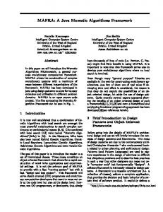
As an example, Fig. 1.2 shows the results for the set of integers {205, 157, 133, 111, 100, 91, 88, 59, 47, 23}. According to the KKH, the numbers 205 and 157 must be assigned to different partitions, and so do 133 and 111. The process is repeated until only one number remains: the value of the partition. If we continue the example, we will have 6 as the weight of the resulting partition.

2.1

A crash introduction to “phase transitions”

An important optimal algorithm that uses KKH is the Complete Karmarkar Karp (CKK) method proposed by Korf (1998). CKK is an exact anytime algorithm which takes advantage of the KKH.

Enhancing MA Performance by Using Matching-based Recombination

5

Figure 1.2. Tree provided by the KKH. Oval nodes go to one partition, and rectangular nodes to the other one. The numbers in brackets are the successive labels assigned to each subtree. The final weight of the tree is 6.

The CKK algorithm is a hard adversary for metaheuristics, particularly due to a phenomenon that in the Artificial Intelligence literature is generally cited as a “phase transition” (Cheeseman et al. 1991). i.e., the transition from a “region” in which almost all instances have many solutions to a region in which almost all instances have no solutions, as the constraints become tighter. This feature is sometimes uncovered by exact algorithms, and can be experimentally —and in some situations even theoretically— analyzed using samples of randomly-generated problems (Mitchell et al. 1992, Mammen and Hogg 1997, Smith and Dyer 1996). Regarding the specific case of the Min Number Partitioning problem and in relationship with the CKK algorithm, it uncovers the “Easyhard-easy” type of transition. We will try to give some intuition on this type of transitions by considering an analogous problem. Suppose for a moment that we are given n stones of different weights (with an average weight W ) and that our task is to separate them in two groups of the same weight. For the “large n” limit (assuming we keep a fixed W ), we can analogously think of the “low W /n” limit, so we can think of the “stones” as grains of sand. It is clear that the task is significantly easier in this case, since the probabilities and combinatorics are playing for us: several optimal solutions may exist, and certainly many suboptimal solutions with costs that are numerically very close to the perfect (optimal) partition value. Also, in the “small n” limit, the problem is also expected to be easy for an exact algorithm, since the search space is greatly reduced. So clearly, there is a relationship between the two magnitudes where the search is expected to be harder. Recurring once again to the intuition of the reader, certainly we do not expect that the existence of a single optimal solution would characterize the particular scenario that would be the hardest for the exact algorithm under consideration. This is clear from the fact that in the “small n”

6 limit we can easily expect to have a single optimal solution, though the problem would be easy (on average) since it has a small number of possible configurations (2n−1 ). Thus we can expect that the problem is harder on average when the number of elements is as large as possible yet it still has a single solution. In this sense, the particular instance of Min Number Partitioning used in Fig. 1.2 was used with a purpose in mind. We have chosen it to illustrate the workings of the KK heuristic since this set of n = 10 numbers {205,157,133,111,100,91,88,59,47,23} is discussed in page 234 of (Papadimitriou 1994). In the author’s own words: “...(notice that their sum, 1014, is indeed less than 2n − 1 = 1023). Since there are more subsets of these numbers than there are numbers between 1 and 1014, there must be two different subsets which have the same sum. In fact, it is easy to see that two disjoint subsets must exist that must have the same sum.”

It is thus clear that the concept behind these “phase transitions” is very intuitive. Although it has been probably identified and discussed well before 1991 (Cheeseman et al. 1991), it has very seldom received the attention it deserves when selecting which instances to use in the computational experimentation with heuristic algorithms and metaheuristics. Curiously, the work of Cheeseman et al. (1991) has been cited a few hundred times in the computing literature, yet most papers in the metaheuristic area do not take into account these facts when selecting the particular instances under study to test their methods. Here we have taken particular care regarding the generation of instances and the behavior of metaheuristics in the three regions which has helped us to understand the characteristics of our methods. It would be interesting to collect evidence on how long the existence of the so-called “phase transitions” (a term borrowed from Physics), has also been reported in the account of experimental studies with exact methods like Branchand-Bound (Lawler and Wood 1966) or Branch-and-Cut (Caprara and Fischetti 1997).

2.2

The IMKK Heuristic

To our knowledge there has been no other heuristic that would allows us to replace the basic KKH scheme with another fast algorithm. We provide one such an attempt, an iterated constructive heuristic that we tentatively named IMKK for Iterated Matching and KKH . For simplicity, we discuss here an implementation of this idea using a greedy matching algorithm. Suppose we have as input the following partition: A1 = {205, 133, 111, 59, 47} and A2 = {157, 100, 91, 88, 23}. Note that the cost associated to

Enhancing MA Performance by Using Matching-based Recombination

7

this partition is |555 − 459| = 96, higher than the one obtained by the KKH for the same instance of Fig. 1.2. Now we proceed constructing a weighted bipartite complete graph G(V, E), such that V = V1 ∪ V2 and V1 and V2 are two independent sets. We have a vertex in V1 for each element of A1 (analogously, we have a vertex in V2 for each element of A2 ). The weight of an edge (vi , vj ) ∈ E between two vertices vi ∈ V1 and vj ∈ V2 , is given by |aj − aj | of the corresponding numbers ai ∈ A1 and aj ∈ A2 . For the given partition, we can run a greedy algorithm that tries to find a matching of minimum weight. Bending a little the notation, this matching can be written as the following list of paired numbers M = {(111, 100), (47, 23), (157, 133), (88, 59), (205, 91)}. The weight of such a matching is 11 + 24 + 24 + 29 + 114 = 202. If we make the heuristic argument that we can assume that the matching can be understood as a constraint that obliges the numbers to be in different partitions, then we can run the KKH on an instance that has half the original size with the numbers {11, 24, 24, 29, 114}. The whole pseudocode is shown in Fig. 1.3. Matching and KKH Algorithm in: partition (A1 , A2 ) out: partition (A01 , A02 ) begin G ← ∅; foreach i ∈ A1 , j ∈ A2 do G ← G ∪ {(i, j)}; M ← FindMatching (G); A0 ← ∅; foreach (i, j) ∈ M do A0 ← A0 ∪ {|i − j|}; (A01 , A02 ) ← KKH (A0 ); end; Figure 1.3. A single step of the IMKK Algorithm. This process can be iterated so as to further improve the output partition.

Following the procedure above we obtain the new partition of the (1) (1) original numbers A1 = {205, 133, 100, 59, 23} and A2 = {157, 111, 91, 88, 47} with an associated cost of |520 − 494| = 26, which is still above the one given by the KKH. Iterating the procedure once again, we obtain the matching M = {(100, 91), (59, 47), (133, 111), (205, 157), (23, 88)}, with weight 9 + 12 + 22 + 48 + 65 = 156. Running the KKH on (2) the set of numbers {9, 12, 22, 48, 65} we obtain the partition A1 = (2) {205, 133, 100, 47, 23} and A2 = {157, 111, 91, 88, 59} which has an as-

8 sociated cost of |508 − 506| = 2, smaller than the one obtained by the KKH alone. We leave as an exercise to the reader what happens if we iterate the procedure another time. However, we can anticipate the result: we obtain again the same matching, and as a consequence, the same result for the KKH. In essence, we are trapped in a “local minimum” 1 of this procedure. This is certainly interesting and it suggests that a procedure based on repeated application of the KKH and a minimum weight matching algorithm on a complete bipartite graph can be used as an engine for a new type of metaheuristics for this problem. This issue is tackled in the next section.

3.

Recombination Approaches Based on Weight Matching

As shown in the previous section, the idea of applying KKH on reduced (via matching) instances of the problem can be a promising mechanism for introducing sensible knowledge about the target problem (Min Number Partitioning in this case) in the search algorithm at hand. While it is still unclear whether its use as search engine in pure localsearch metaheuristics can be useful, it is much more evident that this technique can provide very useful guidelines to model information exchanges in population-based-search metaheuristics such as evolutionary algorithms (EAs). More precisely, the inclusion of problem knowledge into the EA by means of heuristic procedures such as this will result in a memetic algorithm (Moscato 1989, Moscato and Norman 1992) (MA henceforth). A general description of these techniques will be given in Section 1.4. Previously, this section is devoted to discuss the utilization of weight-matching ideas within recombination, a key component in MAs by which a new solution is created by combining information from a set (usually a pair) of existing solutions. In this sense, two main approaches are identified: the use of minimum matchings, and the utilization of balanced matchings.

3.1

Minimum-Weight-Matching Recombination

The approach discussed in this subsection is very similar to the plain IMKK algorithm presented before. The pseudocode is shown in Fig. 1.4. The following example may be useful to illustrate the actual functioning of this pseudocode. Suppose we are given the two parental solutions S1 = {205, 133, 47, 23}{157, 111, 100, 91, 88, 59} and S2 = {205, 111, 100}{157, 133, 91, 88, 59, 47, 23} having costs of |408 − 606| = 198 and |416 − 598| = 182; we first start by constructing the graphs as-

Enhancing MA Performance by Using Matching-based Recombination

9

Minimum Weight-Matching Recombination in: partitions (A1 , A2 ), (A01 , A02 ) out: partition (A001 , A002 ) begin G1 ← ∅; G2 ← ∅; foreach i ∈ A1 , j ∈ A2 do G1 ← G1 ∪ {(i, j)}; foreach i ∈ A01 , j ∈ A02 do G2 ← G2 ∪ {(i, j)}; M ← G1 ∩ G2 ; foreach i ∈ A1 ∪ A2 do M ← M ∪ {(i, 0)}; M 0 ← OrderedList(M ); (i, j) ← FindFirst (M 0 , max(A1 ∪ A2 )); E ← {i, j}; A ← {|i − j|} while E 6= A1 ∪ A2 do DeleteAllOccurrences (M 0 , i); DeleteAllOccurrences (M 0 , j); (i, j) ← GetNextEdge (M 0 , M ); // (i, j) ∈ M 0 and minimizes // max{||i − j| − |k − l|| |(k, l) ∈ M, (k, l) ∈ / M 0} E ← E ∪ {i, j}; A ← A ∪ {|i − j|} endwhile (A001 , A002 ) ← KKH (A); end; Figure 1.4.

The Minimum Weight-Matching Recombination.

sociated with them as mentioned above. We then identify common edges, i.e., pairs of numbers being in different partitions in both solutions. Sorting this list according to edge weights yields in this example: (133, 111) = 22, (133, 100) = 33, (205, 157) = 48, (100, 47) = 53, (111, 47) = 64, (100, 23) = 77, (111, 23) = 88, (205, 91) = 114, (205, 88) = 117, and (205, 59) = 146. The next step is augmenting this list with edges connecting each number with a dummy element ‘0’. The rationale behind this is that it could better to consider a number in isolation rather than taking a bad matching from the parents. In this example, we obtain: (133, 111) = 22, (23, 0) = 23, (133, 100) = 33, (47, 0) = 47, (205, 157) = 48, (100, 47) = 53, (59, 0) = 59, (111, 47) = 64, (100, 23) = 77, (111, 23) = 88, (88, 0) = 88, (91, 0) = 91, (100, 0) = 100, (111, 0) = 111, (205, 91) = 114, (205, 88) = 117, (133, 0) = 133, (205, 59) = 146, (157, 0) = 157, and (205, 0) = 205. Now, we find the first appearance of the highest number (205), and mark the corresponding edge (205, 157) whose weight is 48. Next, we

10 proceed iteratively by considering the edge that minimizes the largest weight difference with respect to an already marked edge, and whose members (excluding the ‘0’ if it were the case) are not included in any marked edge. This process is repeated until all numbers are included in one marked edge. In our example, edges would be marked in the following order: (205, 157), (0, 47), (0, 59), (133, 100), (0, 23), (0, 88), (0, 91), (0, 111). The whole process till this point has been devoted to extract some common information from the parents. We now need to use this information to create a new solution. This is done by running the KKH using the edge weights. In our example we obtain the partition {111, 59, 47, 33} {91, 88, 48, 23} that translates into the final partition {157, 133, 111, 59, 47}{205, 100, 91, 88, 23} whose cost is 0.

3.2

A recombination algorithm based on finding a balanced matching

After some initial experimentation with the recombination algorithm based on minimum weight matching, we recognized that a variant of the original idea may be more useful for this problem. Again we will resort to our favorite instance example to explain this method. Using the example discussed in Subsection 1.3.1, we have two parental partitions S1 = {205, 133, 47, 23} {157, 111, 100, 91, 88, 59} and S2 = {205, 111, 100}{157, 133, 91, 88, 59, 47, 23} having costs of |408 − 606| = 198 and |416 − 598| = 182. As we did before, we construct an undirected graph with edge weights given by (133, 111) = 22, (23, 0) = 23, (133, 100) = 33, (47, 0) = 47, (205, 157) = 48, (100, 47) = 53, (59, 0) = 59, (111, 47) = 64, (100, 23) = 77, (111, 23) = 88, (88, 0) = 88, (91, 0) = 91, (100, 0) = 100, (111, 0) = 111, (205, 91) = 114, (205, 88) = 117, (133, 0) = 133, (205, 59) = 146, (157, 0) = 157, and (205, 0) = 205. Now we can search for the most balanced matching in the graph, that is, a matching that minimizes the absolute difference between the weights of the heaviest and lightest edge in the matching. Instead, to avoid the computational complexity associated to performing this operation, we resort to a simpler heuristic. Since we have 20 edges, we start by considering the tenth edge in the increasing order, which is (111, 23) = 88. Selecting this edge means that we have already decided that the numbers 111 and 23 go in different sides of the partition. They are both marked. We next consider the two consecutive edges in the order. Integers 23 and 111 are already marked, so the next edges to consider are (59, 0) = 59 and (88, 0) = 88. At each step, we will greedily take

Enhancing MA Performance by Using Matching-based Recombination

11

the edge that minimizes the current imbalance of the matching. In this case (88, 0) = 88. We mark 88 and proceed, now with (59, 0) = 59 and (91, 0) = 91. We select (91, 0) = 91, mark 91, and continue, now selecting (100, 0) = 100, and so on. We end this procedure when all the integers are marked and we have a matching. We then run the KK heuristic, passing as input the set of weights of the edges. The resulting solution is then used to create the actual partition for the original numbers. Thus, the main difference with respect to the previous recombination algorithm is the fact that GetNextPair (M 0 , M ) returns a pair (i, j) ∈ M 0 that minimizes max(a, b), where a = ||i − j| − max{|k − l| | (k, l) ∈ M, (k, l) ∈ / M 0 }| and

(1.3)

b = ||i − j| − min{|k − l| | (k, l) ∈ M, (k, l) ∈ / M 0 }|,

(1.4)

rather than simply minimizing max{||i − j| − |k − l|| | (k, l) ∈ M, (k, l) ∈ / M 0 }.

4.

(1.5)

The Memetic Algorithm

As mentioned before, the recombination operators already described will be integrated within a problem-adapted evolutionary algorithm, also known as hybrid evolutionary algorithm (Davis 1991) or memetic algorithm (Moscato 1989). Besides the utilization of these smart recombination operators, MAs use additional mechanisms in order to include problem-specific knowledge into the search engine. A general view of these mechanisms is provided in Subsection 1.4.1. Subsequently, the particular details for adapting the generic components described in this first subsection to the target problem will be discussed in the next subsections.

4.1

Pseudocode for memetic algorithms

The particular MA used in this work is the so-called Local-Searchbased MA, a population-based-search algorithm that intensively uses local search in order to boost solution quality (see the pseudocode in Fig. 1.5). This use of local search motivates a view of the process in which each solution is an agent that tries to improve its quality, cooperating and competing with other agents in the population (Norman and Moscato 1991, Slootmaekers et al. 1998). This generic template can have a huge variety of instantiations. For instance, the FirstPop() function can generate a set of random solutions for the problem at hand, or use a construction heuristic (or a set of

12 Local-Search-based Memetic Algorithm begin P op ← FirstPop(); foreach agent i ∈ P op do i ← Local-Search-Engine(i); EvaluateSolution(i); endfor repeat /* generations loop */ for j ← 1 to #recombinations do Spar ← SelectToMerge (P op); of f spring ← Recombine(Spar , x); of f spring ← Local-Search-Engine(of f spring); EvaluateSolution(of f spring); AddInPopulation (of f spring, P op); endfor; for j ← 1 to #mutations do i ← SelectToMutate (P op); im ← Mutate(i); im ← Local-Search-Engine(im ); EvaluateSolution(im ); AddInPopulation (im , P op); endfor; P op ← SelectPop(P op); if Converged(P op) then P op ← RestartPop(P op); until termination-condition; end; Figure 1.5.

The Local-Search-Based Memetic Algorithm

them if more than one is known) in order to generate a set of good initial solutions. As to the Local-Search-Engine() function, it receives as input a solution and applies an iterative improvement algorithm to it. This improvement algorithm iterates until it is no longer possible to improve the current solution or it is judged not probable to achieve further improvements. Note that in many circumstances, there is no need to evaluate the guiding function2 (using the EvaluateSolution() algorithm) until we got the final solution (the Local-Search-Engine() may be capable of determining whether a certain modification to the current solution is acceptable by using heuristic knowledge about the target function).

Enhancing MA Performance by Using Matching-based Recombination

13

After the initial population has been created, at least one recombination is done. Some MAs ask all the solutions to be involved in recombinations, so #recombinations is fixed and does not need to be specified as a numerical parameter. The SelectToMerge() function is executed by selecting a subset of k solutions to be used as input of the k-merger , a k-ary recombination procedure. Some MAs use a random function, while others use some more complex approach. For instance, there are authors who also advocated for the benefits of using a population structure for interaction of agents (Gorges-Schleuter 1989, M¨ uhlenbein 1991, Gorges-Schleuter 1991, Moscato 1993). A new solution is created by recombining the selected solutions according to the Recombine() function. This can start a variety of procedures, ranging from a single application of any available efficient (i.e., polynomial-time) k-merger algorithm up to more complex recombination operators (which means that they need not be efficient) such as the more systematic searches proposed by Aggarwal et al. (1997) as well as the one used in the recent GAs proposed by Balas and Niehaus (1996). Afterwards, it is optimized and added (or not) to the population according to some criteria. Analogously, a number of solutions are subjected to some mutations. Sometimes the Mutate() function is implemented as a random process, but this is not the general rule and other forms of mutation are possible. Again, the solution is re-optimized at the end of the mutation process and added or not to the population. The SelectPop() function will act on the population, having the effect of reducing its size. The selection of this subset is not always determined by the objective or the guiding function. It may be biased by other features of the solutions, like the interest of maximizing some measure of diversity of the selected set. Again, this can be implemented in a variety of ways. The convergence of the population is sometimes decided by reference to a diversity-crisis, a measure which indicates, below a certain threshold, that the whole population has very similar configurations. When the population has converged, a RestartPop() function is used. In general, the best solution found so far (or incumbent solution) is preserved and a new population is created using some randomized procedure. All the solutions of the population are optimized and evaluated afterwards and the whole process is repeated. The termination-condition can also be implemented in many ways. It can be a time-expiration or generation-expiration criteria as well as more adaptive procedures, like some dynamic measure of lack of improvement.

14

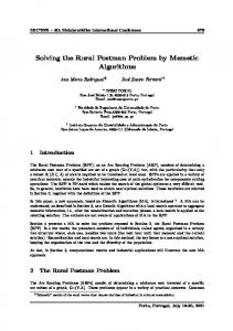
Figure 1.6. Population structure (a complete ternary tree) used in all the MAs in this study on the Min Number Partitioning problem.

4.2

Representation and Search Space

In this paper, we have used the direct representation (Ruml et al. 1996) which is complete since it can generate all possible partitions (the associated search space has 2n configurations, two for each solution of the problem). In this representation, a partition (A1 , A2 ) is represented as a signed bit array {ai | 1 ≤ i ≤ |A1 ∪ A2 |}, where ai = 1 if the ith element of A1 ∪A2 (under an arbitrary but fixed enumeration) belongs to A1 , and ai = −1 otherwise. We will note that any solution is represented by two configurations (s, s0 ∈ S). For instance s = {1, −1, −1, 1, −1, −1} and s0 = {−1, 1, 1, −1, 1, 1} both represent the same partition (i.e., the same solution) of six integers. Another representation that can be used for this problem is called ternary direct since it allows alleles to take one out of three different values, ‘0’, ‘1’, or ‘−1’. Obviously, the associated search space is also complete since it contains the search space of the direct representation. These two representations were studied using a variety of MAs in (Berretta and Moscato 1999). We have kept the best MA of that work (an MA using the direct representation) as benchmark metaheuristic. The aim here would be to see if those results can be improved by other new heuristic ideas for the recombination methods.

4.3

Population size and structure

The population has a fixed size of 13 agents, arranged with a neighborhood relationship based on a complete ternary tree of three levels (See Fig. 1.6). Initially chosen for historical reasons, this structure has revealed itself as very appropriate with respect to the implementation of behaviors, a topic discussed in Subsection 1.4.5.1

Enhancing MA Performance by Using Matching-based Recombination

15

Such interaction topology can be interpreted as a variant of island models (Tanese 1989) of evolutionary algorithms, in which each subpopulation has four agents, one “leader” node and three “supporters”. The latter are one level below in the hierarchy, so agent 1, the root of the tree, is the leader of the top subpopulation and has as supporters agents 2, 3, and 4. Agent 2 has as supporters agents 5, 6, and 7, etc. Note that agents 2, 3, and 4 play both leader and supporter roles. Each agent of the population is handling two feasible solutions, configurations of the associated search space. One is named “Pocket” and the other one “Current”. Whenever the Current solution of an agent has a better guiding function than the Pocket solution, they are switched. We can understand the Pocket as playing the role of a “memory” of past good solutions. Another procedure named PocketPropagation changes two Pocket solutions if the leader has a Pocket solution which is worse than one of its followers. We only require these two mechanisms to guarantee the flow of better solutions towards the agent at the top of the hierarchy. In our MAs, agents optimize their Current configurations/solutions with periods of local search which alternate with recombination. For this particular implementation of an MA, we choose to call as one generation the process in which agents have evolved their Current solutions to be local minima and afterwards they engage in recombination (in total agreement with the pseudo-code that we presented earlier).

4.4

The FirstPop() function

The FirstPop() function creates 13 agents, each with a Pocket and Current configuration representing a partition (A1 , A2 ). All solutions are represented using the direct representation, and are chosen with equal probability.

4.5

The Recombine() procedures

We have used the complete ternary tree neighborhood topology for interaction between agents. As a consequence, we oblige supporters to recombine with their leaders only. The population structure and this rule suggest that the island models of GAs (taken as a metaphor for evolution with colonization and diffusion) is not the most representative for this MA. Instead, the approach might resemble a hierarchical organization in which “communication of ideas” or “exchange of information” can only occur with the immediate leader member of a subgroup. At each generation step, the Current solution of each agent is replaced which a new one generated by the Recombine() procedure acting on the

16 Pocket solution of the supporting agent and its leader. For example, the Current of the agent 2, in Fig. 1.6, will be replaced by the output of the Recombine() procedure having as input the Pocket of agent 1 and the Pocket of agent 2; the Current of agent 9, will be replaced by the Recombine() using the Pocket of agent 3 and the Pocket of agent 9; etc. Then, all agents except agent 1 will replace its Current solution in one iteration of the generation loop. Regarding the previous pseudocode, the number #recombinations performed at each generation step is 12. Moreover, the SelectToMerge() function can be regarded as totally constrained , since each agent always engage in recombination with the same agents.

4.5.1 Behaviors. Before a leader recombines its solution with any of its three supporters, a different type of behavior is assigned to each one. A behavior can be understood as one extra control parameter in the control set of a given recombination operator (Radcliffe and Surry 1994b). Each supporter will have different behavior, which will be decided randomly with equal probability. The three types of behaviors used will be described below. To simplify the presentation, let us suppose that the direct representation is being used, and parent P1 is the leader and the parent P2 is one of the supporters. behavior rebel conciliator obsequent Table 1.1.

first copied in the offspring alleles of P2 which are different from P1 alleles in common to P1 and P2 alleles of P1 which are different from P2

Different behaviors in leader/supporter recombination.

For instance if P1 = {−1, −1, 1, −1, 1} and P2 = {1, −1, 1, 1, −1} are the parents, the recombination using the same parents as input and each type of behavior occurs as follows: the ‘x’ stands for a value that will be decided by algorithms which we will explain at a later stage, then, rebel conciliator obsequent

{1 {x {-1

x -1 x

x 1 x

1 x -1

-1} x} 1}

The conciliator behavior is an example of a recombination procedure that respects the representation (Radcliffe and Surry 1994a, Radcliffe 1994) since “every child it produces contains all the alleles common to its two parents” (i.e., those in A ∩ B). It shares the property of being a respectful recombination as it is also the case of uniform crossover .

Enhancing MA Performance by Using Matching-based Recombination

17

In this case, since all alleles not in A ∩ B have either the value ‘−1’ or ‘1’, the recombination with conciliator behavior is said also to transmit alleles since “each allele in the offspring is present in at least one of its parents”. Both the rebel and the obsequent behaviors do not respect (in the sense postulated by Radcliffe) binary representations since they may exclude allele values in A ∩ B. Analogously, these behaviors are nontransmitting, since it is allowed to create allele values not present in any parents. In order to decide the positions in the offspring where no allele was chosen (the ‘x’ marks) we have investigated several different variants. For the direct representation, three types of algorithms have been used: generalized transmission (GT ), GT with greedy repairing (GTgr ), and GT random seeded - greedy repairing (GTrsgr ). The GT decides at random between either ‘−1’ or ‘1’ with equal probability. The GTgr uses a greedy algorithm, i.e., a deterministic rule which sequentially decides between ‘−1’ or ‘1’ in order to minimize the actual imbalance. The order is based in a non-decreasing order of the sequence of not yet decided integers. The GTrsgr starts by randomly selecting a gene for which its allele value has to be decided. After giving this gene a values minimizing the imbalance, GTrsgr continues in a deterministic way as the GTgr does. According to the definitions given in (Moscato 1999), all of them are crossover operators (can be performed in O(n log n) time), while the GT is the only blind one, since it does not use information from the instance of the problem. To further illustrate the functioning of these “patching” algorithms, consider the instance A = {15,12,10,9,4} and the two parents P1 and P2 mentioned above with conciliator behavior. The offspring first receives the common allele values, i.e., O = {x,−1,1,x,x}. With GT , each ‘x’ will be decided at random with the same probability (in this case we have the traditional uniform crossover . With GTgr , we chose O[1]=1, O[4]=−1 and O[5]=−1, in this order. Note that in this case we decided for ‘1’ or ‘−1’ accordingly to the actual absolute difference of the partial partition. With GTrsgr we might start by making O[4]=1, followed by O[1]=−1 and O[5]=1.

4.6

The Mutate() procedures

We have implemented two types of mutations, Simple and Minimal . The Simple mutation receives as input a solution and for all allele values it decides whether to “flip” it (change from ‘−1’ to ‘1’ or from ‘1’ to ‘−1’) with a fixed probability of 0.1.

18 The Minimal mutation was inspired in the Binomial Minimal Mutation as discussed in (Radcliffe and Surry 1994b). However, we refer to that paper for inspiration only, as a remarkable difference exists. In our case we have taken into account the characteristics of the objective function (to which the label ‘minimal’ actually refers in this case): alleles will not have its sign changed with the same a priori probability used by the Simple mutation (i.e., 0.1). Let us suppose allele i has sign vi = 1 and has been selected to be mutated. Let us also suppose we have represented the solutions with the traditional signed bit array, such that the indexing corresponds with a non-increasing order of the integers of the instance A3 . We then proceed to identify the index of the first allele in the “left direction” (referring to the array) jl and the first allele in the “right direction” jr which have different signs (vjr = vjl = −1). Then vjl is the allele value of the smallest integer which is higher or equal than integer ai and assigned to a different partition. Analogously, vjr is the allele of the largest integer which is smaller or equal to integer ai but in a different partition. Then we select which one of jr and jl minimizes |ai − aj |. We then swap its allele value with the value of vi . We can then say, analogously to the recombination procedures, that the Simple mutation is a blind operator while the Minimal mutation is not since it uses information of the objective function (Moscato 1999, Moscato and Cotta 2002).

4.7

The Local-Search-Engine() procedures

We have implemented two different types of local search algorithms. One was called GreedyImprovement and the other one was called TabuImprovement. For both of them, the input is one solution, and the output is a solution with the same or better objective function value mP (y, x). Using the GreedyImprovement we start by selecting one allele i at random. Then, as we did with the minimal mutation, we identify the position of the first allele in the “right” direction (jr ) and the position of the first allele in the “left” direction (jl ) such that vjr = vjl 6= vi (it may be possible to find only one satisfying the condition). We decide to swap the values of vi with either vjl or vjr if the objective function value (mP (y, x)) is reduced. If both can do that, we chose the one that causes the largest reduction. We repeat this process until (F ailuresT ries − SuccessT ries) > M axN umberOf T ries. Where SuccessT ries is the number of tries that causes better mP (y, x) value and F ailuresT ries count the opposite. We have used several values of the parameter M axN umberOf T ries and we will comment on it later.

Enhancing MA Performance by Using Matching-based Recombination

19

The TabuImprovement uses the same idea of GreedyImprovement. The difference is that in this case we use a basic Tabu Search metaheuristic (Glover and Laguna 1997) inside of the GreedyImprovement. Each swap done between i and j, a tabu matrix (T ABU ) of integers stores, in the position T ABU [i][j], the number of trials that the swap between i and j will be ‘tabu’. In TabuImprovement we can allow swaps which do not reduce the value of mP (y, x), but the output of this procedure is the configuration with the best mP (y, x) found. We repeat this process until (F ailuresT ries−SuccessT ries) > M axN umberOf T ries. In this case, the variable SuccessT ries is the number of tries that could be done, i.e., the number of times a try was not tabu. In addition, we use a simple aspiration criteria (Glover and Laguna 1997). If a swap causes a improvement in the objective function that has never been reached before, we do this swap, even it was declared ‘tabu’.

4.8

RestartPop()

During the evolution of the population, agents recombine only within its subpopulation. More specifically, an agent only recombines its Pocket solution with the one that its leader has. A “diversity crisis” can then happen when three supporters of the same subpopulation all have very similar configurations. Obviously, it is necessary to provide a precise definition of similarity in order to formally establish when a diversity crisis is taking place. The criterion we used to define a diversity crisis is the following: we select at random 20% of the allele values of the Current solution of the three supporters; if the three solutions have the same values in these alleles, then a diversity crisis happened. When a diversity crisis is detected, the leader will not recombine with its three supporters, but the three supporters will recombine with supporters which belong to different subpopulations. For example, in general, agent 2 recombines with its three supporters, i.e., agents 5, 6 and 7. Whenever a diversity crisis is detected (i.e., agents 5, 6, and 7 have similar configurations), the recombination will be done between {5, 6, and 7} and {8, 9, and 10} or between {5, 6, and 7} and {11, 12, and 13}. Three recombinations will modify the Current solutions of agents 5, 6, and 7; i.e., if it was chosen {5, 6, and 7} and {8, 9, and 10} (this second subpopulation was randomly selected), the recombination pairs can be: 5 with 9, 6 with 10, and 7 with 8. The assignments are chosen at random too. As a consequence, we may get some extra diversity.

20

4.9

Lack of improvement

We have also investigated a rule for lack of improvement. In the context of this problem, the results have been very promising. We have introduced a very simple rule: if after three consecutive generations there is no improvement of the incumbent solution in the population (i.e., if the Pocket solution of the agent at the top of the hierarchy has not been updated), we save the solution (for the off-line assessment of the algorithm), we eliminate it from pocket 0 and we set it to a randomly created solution.

5.

Tabu Search

The Tabu Search heuristic implemented in (Berretta and Moscato 1999) was used in that work as a kind of “background” operator. It was introduced rather for being in charge of diversifying the search than for providing improved solutions. However, it used the “minimum” neighborhood, meaning that it is analogous to the minimum mutation as explained in that chapter. This is a severe drawback since it means that, given a solution, we only move to other solutions that have the same number of elements in each side of the partition. This said, it is the case that a more powerful neighborhood must be used to improve the search, allowing to change the cardinalities of the two subsets. Given the good results of this Tabu Search implementation, but aiming to provide a larger neighborhood that would free it from being “cardinality constrained”, we have added another Tabu Search procedure that interleaves with the former one. We have named it “exhaustive”: for each allele value, we compute the cost of reversing its sign, i.e., to move the associated integer to the other side of the partition; we perform the change that maximizes the reduction in cost, or the one that minimizes the increment if no decreasing change is available. These two search strategies are alternatively executed during a single Tabu Search individual optimization step. Since the “exhaustive” method requires more computer time, we make it run for a shorter period than the other one. More precisely, TS runs for k steps using the minimum neighborhood, and for k/10 steps using the exhaustive neighborhood, where k is one tenth of the total number of allowed TS steps. Note that both Tabu Search strategies have their own different attribute lists. For the “minimum” TS strategy, an attribute is a pair (i, j) while for the the “exhaustive” scheme it is just the i that corresponds to the integer than has changed. The time an attribute remains tabu is the same as in (Berretta and Moscato 1999), i.e., a uniformly distributed integer random number in [1, n].

Enhancing MA Performance by Using Matching-based Recombination

6.

21

Computational results

We have studied three groups of instances. In each group the integers have 10, 12, and 14 decimal digits respectively. We also note that the instances with 10 decimal digits where the same as the one used in (Berretta and Moscato 1999) to help us evaluate the benefits, if any, of the new ideas tested in this work. Again, we have taken extreme care with the generation of the instances, and the best approach has been to generate each decimal digit of each integer of each instance uniformly at random to avoid any spurious correlations. In each group we have 100 instances, with n = 15, 25, 35, . . . , 105 integers. This means that we have 10 independently generated instances for each value of n. Table 1.2 shows the results of the KKH on these instances. Results for the complete KK algorithm are also included for the smallest test instances. n 15 25 35 45 55 65 75 85 95 105 mean (≥ 35)

CKK (D=10) 1785469 3161 3 1 1 1 1 0 1 0 1

KKH (D=10) 62529719 2087226 422345 329255 97390 15250 20488 3386 3122 1656 111612

KKH (D=12) 11143286419 409925198 44169859 20000541 7841909 2541069 464585 1249715 290572 261532 9602473

KKH (D=14) 284759439645 27573832748 7557306861 3308094310 833784155 81996483 205571875 23506635 45466008 21748182 1509684313

Table 1.2. The performance of CKK and KKH on the three sets of instances (CKK could only be run on instances with 10 digits).

We have first run a Tabu Search algorithm for 109 iterations. It is important to remark that this Tabu Search algorithm is different to the one implemented in (Berretta and Moscato 1999). This implementation obtains better results than the one that uses the “minimum” neighborhood described in (Berretta and Moscato 1999). The results for this improved Tabu Search algorithm are shown in Table 1.3. The memetic algorithms have been run for 5,000 generations, which approximately corresponds to the same time employed by the Tabu method. The results obtained are shown in Tables 1.4, 1.5 and 1.6. With MA-behavior, we denote the best memetic algorithm that has been reported in (Berretta and Moscato 1999), i.e., it uses behavior-based recombination but the same restart mechanism that has been described in this paper. With MA-matching, we denote the same memetic algorithm

22 n 15 25 35 45 55 65 75 85 95 105 mean (≥ 35) Table 1.3.

Tabu (D=10) 1785469 3161 11 11 6 12 6 6 6 4 8

Tabu (D=12) 190858470 243962 926 771 1027 825 478 602 301 328 657

Tabu (D=14) 18097490259 24534199 209194 57018 42114 50144 77951 52960 34633 26581 68824

The performance of Tabu Search on the three sets of instances.

n 15 25 35 45 55 65 75 85 95 105 mean (≥ 35)

Propagate after mutation MA-behavior MA-matching 1785469 1785469 3161 3161 9 16 7 7 5 11 5 4 1 4 5 6 3 5 3 3 5 7

Propagate before mutation MA-behavior MA-matching 1785469 1785469 3161 3161 20 12 7 5 7 2 4 4 3 2 2 4 3 3 3 2 6 4

Table 1.4. The performance of the four MA variants tested on instances with 10 decimal digits. The best results are shown in boldface.

that uses restart, but with the difference that the new recombination algorithm based on finding a balanced matching was used. A variant of each of these MAs has been considered: if, after a recombination, the resulting solution is better than its pocket solution then it is immediately substituted. Note that in the original algorithm we might first introduce a mutation, before the actualization of pockets is tested. We have observed that this small change in the algorithm resulted in a better performance of the balanced matching recombination method, since in this case the creation of a better offspring solution —i.e., better than its parents— seems to happen more frequently than in the behavior-based approach.

Enhancing MA Performance by Using Matching-based Recombination

n 15 25 35 45 55 65 75 85 95 105 mean (≥ 35)

Propagate after mutation MA-behavior MA-matching 190858470 190858470 243962 243962 2355 1667 545 665 672 646 837 715 696 433 465 501 540 388 271 604 798 702

23

Propagate before mutation MA-behavior MA-matching 190858470 190858470 284877 243962 1026 875 1524 284 563 296 269 360 393 443 361 347 201 219 370 478 588 413

Table 1.5. The performance of the four MA variants on instances with 12 decimal digits. The best results are shown in boldface.

n 15 25 35 45 55 65 75 85 95 105 mean (≥ 35)

Propagate after mutation MA-behavior MA-matching 18097490259 18097490259 22076988 22076988 64093 181249 158327 39284 64027 97166 53855 67961 34295 55204 25623 37645 40189 26460 29501 34264 58739 67404

Propagate before mutation MA-behavior MA-matching 18097490259 18097490259 22076988 22076988 58548 86491 95513 30868 36719 50294 66396 45443 45654 40678 58598 35035 39309 21692 37409 19731 54768 41279

Table 1.6. The performance of the four MA variants on instances with 14 decimal digits. The best results are shown in boldface.

From the inspection of these tables we can conclude that the new Tabu Search method has certainly improved over the one presented in (Berretta and Moscato 1999). It is now able to solve instances with 10 decimal digits and n = 15 and n = 25. However, that is not the case for the 12- and 14-digit instances where it is still defeated by some of the new memetic counterparts. The general improvement over the previous methods is clear.

24

7.

Discussion and Future Work

The computational results obtained are consistent with our a priori analysis of weight-matching recombination: on average, the MA with the matching-based recombination (plus the new pocket-propagation strategy) tends to be the best or the second best approach in almost all groups of instances tested. Nevertheless, we believe that a point of caution has to be introduced. We have developed, at a great effort, a new recombination algorithm based on finding an almost perfectly balanced matching. This has resulted in a new memetic algorithm, which can be generalized to introduce the concept of behaviors, and that has already improved over the best methods we have previously developed for this problem. However, a simple rule that we have introduced in the previous scheme had a significant impact on the final performance. Moreover, we believe that —for this particular problem and this particular type of instances— the performance gain obtained when using a population-based approach does not compensate the cost of coding such a complex method as an MA if we have some other alternatives, like the CKK method or a simple Tabu Search scheme. In our opinion, this is an important conclusion that raises once again the “killing flies with a gun” issue. Knowing that no technique is better than any other one in an absolute sense (a crucial fact that the “No Free Lunch” Theorem (Wolpert and Macready 1997) popularized, but that antedates this result), interdisciplinarity and crossbreeding reveal themselves as the necessary strategies for selecting the appropriate technique for a given problem. In any case, the really positive results of this type of “balanced matching recombination” indicate that it is a useful and promising idea, that deserves to be further explored in the future. As mentioned in the introduction, there are several real world problems that can be assimilated to the MNP. The enhanced capabilities of Tabu-based MAs endowed with this recombination scheme can be crucial for tackling these problems.

Bibliography C.C. Aggarwal, J.B. Orlin, and R.P. Tai. Optimized crossover for the independent set problem. Operations Research, 45(2):226–234, 1997. M.F. Arguello, T.A. Feo, and O. Goldschmidt. Randomized methods for the number partitioning problem. Computers & Operations Research, 23(2):103–111, Feb. 1996. E. Balas and W. Niehaus. Finding large cliques in arbitrary graphs by bipartite matching. In D.S. Johnson and M.A. Trick, editors, Cliques,

BIBLIOGRAPHY

25

Coloring, and Satisfiability: Second DIMACS Implementation Challenge, volume DIMACS 26, pages 29–51. American Mathematical Society, 1996. R. Berretta and P. Moscato. The number partitioning problem: An open challenge for evolutionary computation ? In D. Corne, M. Dorigo, and F. Glover, editors, New Ideas in Optimization, pages 261–278. McGraw-Hill, 1999. A. Caprara and M. Fischetti. Branch-and-cut algorithms. In M. Dell’Amico, F. Maffioli, and S. Martello, editors, Annotated bibliographies in combinatorial optimization, pages 45 – 63. John Wiley and Sons, Chichester, 1997. P. Cheeseman, B. Kanefsky, and W.M. Taylor. Where the Really Hard Problems Are. In Proceedings of the Twelfth International Joint Conference on Artificial Intelligence, IJCAI-91, Sydney, Australia, pages 331–337, 1991. L. Davis. Handbook of Genetic Algorithms. Van Nostrand Reinhold, New York NY, 1991. F.F. Ferreira and J.F. Fontanari. Probabilistic analysis of the number partitioning problem. Journal of Physics A: Math. Gen, pages 3417– 3428, 1998. F. Glover and M. Laguna. Tabu Search. Kluwer Academic Publishers, Norwell, Massachusetts, USA, 1997. M. Gorges-Schleuter. ASPARAGOS: An asynchronous parallel genetic optimization strategy. In J. David Schaffer, editor, Proceedings of the Third International Conference on Genetic Algorithms, pages 422– 427, San Mateo, CA, 1989. Morgan Kaufmann Publishers. M. Gorges-Schleuter. Explicit Parallelism of Genetic Algorithms through Population Structures. In H.-P. Schwefel and R. M¨anner, editors, Parallel Problem Solving from Nature I, volume 496 of Lecture Notes in Computer Science, pages 150–159. Springer-Verlag, Berlin, Germany, 1991. ISBN 3-540-54148-9. D.S. Johnson, C. R. Aragon, L. A. McGeoch, and C. Schevon. Optimization by simulated annealing: An experimental evaluation; Part II: Graph coloring and number partitioning. Operations Research, 39 (3):378–406, 1991. D.R. Jones and M.A. Beltramo. Solving partitioning problems with genetic algorithms. In R.K Belew and L.B. Booker, editors, Proceedings

26 of the Fourth International Conference on Genetic Algorithms, pages 442–449, San Mateo, CA, 1991. Morgan Kaufmann. N. Karmarkar and R.M. Karp. The differencing method of set partitioning. Report UCB/CSD 82/113, University of California, Berkeley, CA, 1982. S. Kirkpatrick, C.D. Gelatt Jr., and M.P. Vecchi. Optimization by simmulated annealing. Science, 220(4598):671–680, 1983. D. Kirovski, M. Ercegovac, and M. Potkonjak. Low-power behavioral synthesis optimization using multiple-precision arithmetic. In ACMIEEE Design Automation Conference, pages 568–573. ACM Press, 1999. R. Korf. A complete anytime algorithm for number partitioning. Artificial Intelligence, 106:181–203, 1998. M. Laguna and P. Laguna. Applying Tabu Search to the 2-dimensional Ising spin glass. International Journal of Modern Physics C - Physics and Computers, 6(1):11–23, 1995. E.L. Lawler and D.E. Wood. Branch and bounds methods: A survey. Operations Research, 4(4):669–719, 1966. D.L. Mammen and T. Hogg. A new look at the easy-hard-easy pattern of combinatorial search difficulty. Journal of Artificial Intelligence Research, 7:47–66, 1997. S. Mertens. Phase transition in the number partitioning problem. Physical Review Letters, 81(20):4281–4284, 1998. S. Mertens. Random costs in combinatorial optimization. Physical Review Letters, 84(6):1347–1350, 2000. D.G. Mitchell, B. Selman, and H.J. Levesque. Hard and easy distributions for SAT problems. In P. Rosenbloom and P. Szolovits, editors, Proceedings of the Tenth National Conference on Artificial Intelligence, pages 459–465, Menlo Park, California, 1992. AAAI Press. P. Moscato. On Evolution, Search, Optimization, Genetic Algorithms and Martial Arts: Towards Memetic Algorithms. Technical Report Caltech Concurrent Computation Program, Report. 826, California Institute of Technology, Pasadena, California, USA, 1989. P. Moscato. An Introduction to Population Approaches for Optimization and Hierarchical Objective Functions: The Role of Tabu Search. Annals of Operations Research, 41(1-4):85–121, 1993.

BIBLIOGRAPHY

27

P. Moscato. Memetic algorithms: A short introduction. In D. Corne, M. Dorigo, and F. Glover, editors, New Ideas in Optimization, pages 219–234. McGraw-Hill, 1999. P. Moscato and C. Cotta. A gentle introduction to memetic algorithms. In F. Glover and G. Kochenberger, editors, Handbook of Metaheuristics. Kluwer Academic Publishers, Boston MA, 2002. P. Moscato and M. G. Norman. A Memetic Approach for the Traveling Salesman Problem Implementation of a Computational Ecology for Combinatorial Optimization on Message-Passing Systems. In M. Valero, E. Onate, M. Jane, J. L. Larriba, and B. Suarez, editors, Parallel Computing and Transputer Applications, pages 177–186, Amsterdam, 1992. IOS Press. H. M¨ uhlenbein. Evolution in Time and Space – The Parallel Genetic Algorithm. In Gregory J.E. Rawlins, editor, Foundations of Genetic Algorithms, pages 316–337, San Mateo, CA, 1991. Morgan Kaufmann Publishers. M.G. Norman and P. Moscato. A competitive and cooperative approach to complex combinatorial search. In Proceedings of the 20th Informatics and Operations Research Meeting, pages 3.15–3.29, Buenos Aires, 1991. C.H. Papadimitriou. Computational Complexity. Addison-Wesley, 1994. N.J. Radcliffe. The algebra of genetic algorithms. Annals of Mathematics and Artificial Intelligence, 10:339–384, 1994. N.J. Radcliffe and P.D. Surry. Fitness Variance of Formae and Performance Prediction. In L.D. Whitley and M.D. Vose, editors, Proceedings of the Third Workshop on Foundations of Genetic Algorithms, pages 51–72, San Francisco, 1994a. Morgan Kaufmann. N.J. Radcliffe and P.D. Surry. Formal Memetic Algorithms. In T. Fogarty, editor, Evolutionary Computing: AISB Workshop, volume 865 of Lecture Notes in Computer Science, pages 1–16. Springer-Verlag, Berlin, 1994b. W. Ruml. Stochastic approximation algorithms for number partitioning. Technical Report TR-17-93, Harvard University, Cambridge, MA, USA, 1993. available via ftp://das-ftp.harvard.edu/techreports/tr-1793.ps.gz.

28 W. Ruml, J.T. Ngo, J. Marks, and S.M. Shieber. Easily searched encodings for number partitioning. Journal of Optimization Theory and Applications, 89(2):251–291, 1996. R. Slootmaekers, H. Van Wulpen, and W. Joosen. Modelling genetic search agents with a concurrent object-oriented language. In P. Sloot, M. Bubak, and B. Hertzberger, editors, High-Performance Computing and Networking, volume 1401 of Lecture Notes in Computer Science, pages 843–853. Springer, Berlin, 1998. B.M. Smith and M.E. Dyer. Locating the phase transition in binary constraint satisfaction. Artificial Intelligence, 81(1–2):155–181, 1996. G. Sorkin. Theory and Practice of Simulated Annealing on Special Energy Landscapes. Ph.d. thesis, University of California at Berkeley, Berkeley, CA, 1992. R.H. Storer. Number partitioning and rotor balancing. In Talk at the INFORMS Conference, Optimization Techniques Track, TD15.2, 2001. R.H. Storer, S.W. Flanders, and S.D. Wu. Problem space local search for number partitioning. Annals of Operations Research, 63:465–487, 1996. R. Tanese. Distributed genetic algorithms. In J.D. Schaffer, editor, Proceedings of the Third International Conference on Genetic Algorithms, pages 434–439, San Mateo, CA, 1989. Morgan Kaufmann. D.H. Wolpert and W.G. Macready. No free lunch theorems for optimization. IEEE Transactions on Evolutionary Computation, 1(1):67–82, 1997.