16B.6
ENSEMBLE-DERIVED ESTIMATION OF WIND UNCERTAINTY USING A LINEAR VARIANCE CALIBRATION FOR PROBABILISTIC WEATHER APPLICATIONS Walter C. Kolczynski, Jr.* David R. Stauffer Sue Ellen Haupt Aijun Deng Pennsylvania State University, University Park, PA
1. INTRODUCTION The uncertainty in meteorological (MET) predictions is of great interest for a large number of applications, ranging from economic to recreational to public safety. It is therefore important that numerical models and forecasts provide accurate estimates of their uncertainty along with their best or most likely prediction (NRC 2007). One common method for determining this uncertainty is the use of ensembles, with multiple numerical forecasts produced using slightly different initial conditions and/or model parameterizations. The goal of using an ensemble is to span the possible outcomes given the uncertainties in the initial state of the atmosphere, the limited observations and the modeling system (Leith 1974). The mean of the ensemble has also been shown to outperform any individual ensemble member compared to observations (Hamill and Colucci 1997, Stensrud et al. 1999). While ensemble forecasting is a significant step toward forecasting the most likely outcome and the uncertainty in the forecast, the size of operational ensembles is insufficient to fully represent the probability density function (PDF) of possible forecasts. An ensemble capable of doing so is impractical with current computing resources. Therefore, any MET ensemble provides a sampling of the full forecast PDF and any measures of the uncertainty from the ensemble (such as variance) should be evaluated for applicability and calibrated if necessary. Many studies, including Houtekamer et al. (1997), show that most MET ensembles are under-dispersive (the ensemble spread is consistently smaller than the spread in the forecast errors). Several studies attempt to determine a correlation between ensemble spread and some measure of the error for various variables (Kalnay and Dalcher 1987, Murphy 1988, Barker 1991, Houtekamer 1993, Buizza 1997, Hamill and Colucci 1998, Stensrud et al. 1999), but these studies generally find an unacceptably low correlation between spread and errors (Grimit and Mass 2007). Houtekamer (1993) explains this low correlation using a stochastic model that showed that, even in idealized cases, the correlation between ensemble spread and absolute error will not be large. Grimit (2004) proposes that, rather than a simple spread-to-error correlation, a more probabilistic approach should be used to evaluate ensemble * Corresponding Author Address: Walter Kolczynski, Jr. Dept. of Meteorology, Pennsylvania State University, 503 Walker Bldg. State College, PA 16802;
[email protected].
uncertainty. Specifically, Grimit stresses the distinction between forecast error and forecast uncertainty. Because each forecast results in only one realization of the forecast error (one random draw from the forecast PDF), the error of any particular forecast provides little information about the distribution from which it was drawn. However, if the relationship between the spread of the MET ensemble and forecast uncertainty is constant within a sample, we can group multiple samples with similar ensemble variance and use the distribution of the associated group of errors as a measure of the underlying uncertainty in the errors. Grimit (2004) and Grimit and Mass (2007) use an idealized stochastic model that shows a strong linear relationship between ensemble spread and error variance. Kolczynski et al. (2009) uses a similar method derived from Roulston (2005) on low-level wind data from the National Centers for Environmental Prediction Short-Range Ensemble Forecast (NCEP-SREF). Kolczynski et al. (2009) also finds a strong correlation between ensemble variance and error variance, and uses this linear relationship as a calibration (denoted LVC, for Linear Variance Calibration) for wind variance input into an atmospheric transport and dispersion model. However, unlike the Grimit and Mass study using an idealized model, Kolczynski et al. (2009) finds that the slope of the linear fit is less than the ideal value of one, and that the y-intercept is larger than the ideal value of zero (Fig. 1). The study also finds that these parameters change substantially depending on the length of the forecast. When applied to dispersion calculations in a case study, the calibration improves the resulting dispersion forecast in most of the metrics used in the study. This study further explores possible influences on the LVC slope and intercept. This is done using a stochastic model adapted from that used by Houtekamer (1993) and Grimit and Mass (2007). However, this new stochastic model allows the variance of the error distribution and the ensemble distribution to vary from each other, allowing for the creation of “imperfect” ensembles, but in such a manner that a linear relationship between the variances is maintained. Since we are interested in the variances of low-level wind speed for atmospheric transport and dispersion, the new model also uses a Weibull distribution instead of a log-normal distribution as the underlying “climatology”, as a Weibull approximates the climatology of surface (10-m) wind speed (Wilks 2006). Section 2 provides the details of the new stochastic model. Section 3 presents the results of the model for six experiments using an ensemble size of 20, typical of operational MET ensembles. The same six experiments
are then repeated using varying ensemble size for results in Section 4. Conclusions and directions for future work are offered in Section 5. 2. METHODOLOGY In order to investigate the relationship between ensemble variance and error variance, we construct a stochastic model in which we control the variance from which the data are drawn. This will allow us to compare the results of the model directly with the expected values given the underlying distribution. For each simulation, we first generate a random value of “speed” from a Weibull distribution with a shape parameter of 1.8 and a scale parameter of 5.0. We choose this distribution because we are interested in the low-level winds important for atmospheric transport and dispersion, and Kolczynski et al. (2009) focused on low-level winds. The shape and scale parameters fall within the common range of values empirically determined for the distribution of wind speeds. The error distribution and ensemble distribution are then both defined to be normal distributions with a mean of zero and a variance that depends on . The relationship is a simple linear one, with the variance of the errors ( ) defined as
a2 ma si ba and the variance of the ensemble (
e2 me si be
error/ensemble pairs. A modified version of the Linear Variance Calibration (LVC) presented in Kolczynski et al. (2009) is then used to calculate a relationship between the ensemble variance and error variance. First, the error-ensemble pairs are ordered based on the ensemble variance. Then the data are binned into groups of 1000. In each bin, the ensemble variance is averaged to obtain a representative ensemble variance for the bin, and the variance of the errors in the bin is computed. The philosophy is that, if the relationship between ensemble variance and error variance remains constant within the sample, errors from cases with similar ensemble variance should be drawn from similar error distributions. Thus, we can take the variance of the errors from many different realizations and it would be similar to the variance if we could compute it over many errors for the same case. We then perform a linear regression on the mean ensemble variance/error variance pairs for each bin to determine the slope ( ) and intercept of the relationship ( ). Because we specify the underlying distribution, we can also compute the expected LVC slope and intercept algebraically. The slope of the LVC regression ( ) is expected to be
ma me
(1)
mLVC
(2)
and the y-intercept of the LVC regression ( expected to be
) defined as
Using these variances, we pick one number at random from the normal distribution as our observed error, and M numbers from the distribution to serve as our ensemble. This process is repeated onehundred thousand times to create a population of
bLVC ba be
(3)
ma me
) is
(4)
We can compare these theoretical values to those calculated from the simulated data. 3. EXPLORATION WITH ENSEMBLE SIZE OF 20
Figure 1: Scatterplot showing the relationship between error variance and ensemble variance (adapted from Kolczynski et al. 2009). The linear best-fit line (LVC) has a slope of 0.502 and a y-intercept of 3.007.
In order to explore the behavior of the model with typical operational ensemble sizes, we first consider several configurations using a constant ensemble size of twenty members. Each experiment is summarized in Table 1 along with the 20 member ensemble results. Experiments A and B are both “perfect” ensembles, with the ensemble being drawn from a distribution identical to that from which the errors are drawn. The only difference between A and B is that the variances of B are three times bigger than those of A relative to . Experiments C and D explore simple over- and underdispersive cases, with the ensemble being drawn from distributions with three times larger or one third smaller variances, respectively. Experiments E and F demonstrate more complicated relationships, where the variance of the error distribution or ensemble distribution includes a constant. Figure 2 shows the scatterplot and rank histogram from each experiment. The most important result is that the slope calculated using the LVC ( ) is smaller than the slope expected from algebra ( ). Similarly, the y-intercept computed using LVC ( ) is higher than the theoretical value 2 from algebra ( ). However, the R for every
Table 1: Summary of the experimental configuration and corresponding results for an ensemble size of 20. The color of each row corresponds to the color used in Figs. 3 and 4. Exp. A B C D E F
0.1 0.3 0.1 0.3 0.1 0.1
0.0 0.0 0.0 0.0 0.0 0.4
0.1 0.3 0.3 0.1 0.1 0.1
0.0 0.0 0.0 0.0 0.4 0.0
0.94 0.95 0.98 0.96 0.99 0.92
1.00 1.00 0.33 3.00 1.00 1.00
0.71 0.72 0.24 2.15 0.45 0.72
+0.00 +0.00 +0.00 +0.00 - 0.40 +0.40
+0.13 +0.38 +0.13 +0.39 +0.07 +0.52
Figure 2: Relationship of ensemble variance (abscissa) to the error variance (ordinate) for each experiment, using an ensemble size of 20. Insets: rank histogram of each experiment experiment is high (above 0.92), indicating a strong linear correlation between ensemble variance and error variance even though the coefficients of the linear fit do not match the theoretical values. Interestingly, the slope computed by LVC is 72% of the theoretical value for every experiment except E, which is the only one to use an additive constant for the ensemble variance. There also seems to be a functional relationship for the yintercept calculated by LVC, with the LVC y-intercept being larger than the theoretical value for every experiment except E. 4. EXPLORATION OF ENSEMBLE SIZE To investigate the possible effect of ensemble size on the ensemble variance/error variance relationship,
particularly the deviation from theoretical values, we repeat each experiment for a variety of ensemble sizes ranging from five to five thousand (5, 10, 20, 50, 100, 200, 500, 1000 and 5000). This should reveal any sampling limitations due to ensemble size, as well as indicate any fundamental problems with the LVC if it is unable to obtain the theoretical values at very large ensemble sizes. Figures 3 and 4 show the calculated LVC slope and y-intercept respectively for each experiment at varying ensemble sizes. The LVC calculated values of slope and y-intercept for each experiment approach the theoretical value as ensemble size gets larger. This indicates that the deviation from the theoretical values in the experiments when using 20 members is likely due to sample size issues and is not a byproduct of LVC.
Furthermore, the plot shows that much larger ensemble sizes are needed (> 200) in order to obtain the theoretical slope and y-intercept than are currently used operationally. This is an important outcome, because it means that even with a perfect ensemble, the ensemble variance should be calibrated for any ensemble with fewer than several hundred members. Scientists exploring applications of ensemble variance ranging from ensemble generation to its use as a proxy for uncertainty should be mindful of this result.
Kolczynski et al. (2009) in a controlled way using an idealized stochastic ensemble. The results show that the calculated LVC slope and y-intercept deviate substantially from the algebraically-derived values when ensemble size is less than several hundred members for a climatology that follows a Weibull distribution, as is appropriate for surface wind speed. This result implies that ensemble variances, even from otherwise “perfect” ensembles, should be calibrated if ensemble size is less than several hundred members. This study also determined a potential adjustment to the LVC slope and y-intercept for an ensemble size of 20 that accounts for the sampling error caused by limited ensemble size. This adjustment was accurate as long as , the portion of the ensemble variance independent of the forecast value , was zero. Further research may be able to determine a functional form of this adjustment that works for other ensemble sizes. It may also be possible to compute an adjustment that properly incorporates the additive portion of ensemble variance ( ) as well. This would allow the determination of a “best” possible relationship between error variance and ensemble variance of a given ensemble size. Such a “best” relationship could then be a goal in developing ensemble systems so that their variances are “correct”.
Figure 3: Calculated LVC slope for each of the experiments listed in Table 1 using variable ensemble sizes. The theoretical slope is 1 for Exps. A, B, E and F; for Exp. C; and 3 for Exp. D. Data are plotted at ensemble sizes of 5, 10, 20, 50, 100, 200, 500, 1000, 2000 and 5000.
Acknowledgements. We would like to thank our Penn State colleagues Arthur Small, George Young and Naomi Altman for insightful conversations about uncertainty, probability and statistics that were instrumental in evaluating the stochastic model. This work was supported by the Defense Threat Reduction Agency (DTRA) under the supervision of Dr. John Hannan via the L3-Titan/DTRA contract DTRA01-03-D0013. 6. REFERENCES Barker, T.W., 1991: The Relationship Between Spread and Forecast Error in Extended-range Forecasts. Journal of Climate, 4, 733-742. Buizza, R., 1997: Potential Forecast Skill of Ensemble Prediction and Spread and Skill Distributions of the ECMWF Ensemble Prediction System. Monthly Weather Review, 125, 99-119.
Figure 4: Calculated LVC y-intercept for each of the experiments listed in Table 1 using variable ensemble sizes. The theoretical y-intercept is 0 for Exps. A-D; 0.4 for Exp. C; and 0.4 for Exp. D. Data are plotted at ensemble sizes of 5, 10, 20, 50, 100, 200, 500, 1000, 2000 and 5000. 5. CONCLUSIONS This study has explored the relationship between ensemble variance and error variance calculated by the Linear Variance Calibration (LVC) presented in
Grimit, E.P., 2004: Probabilistic Mesoscale Forecast Error Prediction Using Short-Range Ensembles. Ph.D. dissertation, University of Washington, 146 pp. ------ and C.F. Mass, 2007: Measuring the Ensemble Spread-Error Relationship with a Probabilistic Approach: Stochastic Ensemble Results. Monthly Weather Review, 135, 203-221. Hamill, T.M. and S.J. Colucci, 1997: Verification of EtaRSM Short-Range Ensemble Forecasts. Monthly Weather Review, 125, 1312-1327.
------ and ------, 1998: Evaluation of Eta-RSM Ensemble Probabilistic Precipitation Forecasts. Monthly Weather Review, 126, 711-724.
Murphy, J.M., 1988: The Impact of Ensemble Forecasts on Predictability. Quarterly Journal of the Royal Meteorological Society, 114, 463-493.
Houtekamer, P.L., 1993: Global and Local Skill Forecasts. Monthly Weather Review, 121, 18341846.
National Research Council, 2007: Completing the Forecast: Characterizing and Communicating Uncertainty for Better Decisions Using Weather and Climate Forecasts. The National Academies Press, Washington, DC, 124 pp.
------, J. Derome, H. Ritchie, and H.L. Mitchell, 1997: A System Simulation Approach to Ensemble Prediction. Monthly Weather Review, 125, 3297-3319. Kalnay, E. and A. Dalcher, 1987: Forecasting Forecast Skill. Monthly Weather Review, 115, 349-356. Kolczynski, Walter C. Jr., D.R. Stauffer, S.E. Haupt and A. Deng, 2009: Ensemble Variance Calibration for Representing Meteorological Uncertainty for Atmospheric Transport and Dispersion Modeling. Journal of Applied Meteorology and Climatology, in press. Leith, C.E., 1974: Theoretical Skill of Monte Carlo Forecasts. Monthly Weather Review, 102, 409-418.
Roulston, M.S., 2005: A Comparison of Predictors of the Error of Weather Forecasts. Nonlinear Processes in Geophysics, 12, 1021-1032. Stensrud, D.J., H.E. Brooks, J. Du, M.S. Tracton and E. Rogers, 1999: Using Ensembles for Short-Range Forecasting. Monthly Weather Review, 127, 433-446. Wilks, D.S., 2006: Statistical Methods in the Atmospheric Sciences, Second Ed. Academic Press, Burlington, MA, 627 pp.