2586
MONTHLY WEATHER REVIEW
VOLUME 131
Ensemble Filtering for Nonlinear Dynamics SANGIL KIM Department of Mathematics, The University of Arizona, Tucson, Arizona
GREGORY L. EYINK Department of Mathematical Sciences, The Johns Hopkins University, Baltimore, Maryland
JUAN M. RESTREPO Department of Mathematics, The University of Arizona, Tucson, Arizona
FRANCIS J. ALEXANDER
AND
GREGORY JOHNSON
CCS-3, Los Alamos National Laboratory, Los Alamos, New Mexico (Manuscript received 9 December 2002, in final form 30 April 2003) ABSTRACT A method for data assimilation currently being developed is the ensemble Kalman filter. This method evolves the statistics of the system by computing an empirical ensemble of sample realizations and incorporates measurements by a linear interpolation between observations and predictions. However, such an interpolation is only justified for linear dynamics and Gaussian statistics, and it is known to produce erroneous results for nonlinear dynamics with far-from-Gaussian statistics. For example, the ensemble Kalman filter method, when used in models with multimodal statistics, fails to track state transitions correctly. Here alternative ensemble methods for data assimilation into nonlinear dynamical systems, in particular, those with a large state space are studied. In these methods conditional probabilities at measurement times are calculated by applying Bayes’s rule. These results show that the new methods accurately track the transitions between likely states in a system with bimodal statistics, in which the ensemble Kalman filter method does not perform well. The proposed new ensemble methods are conceptually simple and potentially applicable to large-scale problems.
1. Motivation and model The problem of data assimilation is to determine the best estimate of the solution history of a dynamical system given some partial and inaccurate measurements. The filtering problem is defined as that of estimating the present state given prior observations. It is generally accepted that the optimal solution is obtained by calculating the conditional statistical distribution P[x, t | R (t)] of the state vector x of the system given the set R (t) of measurements up to the current time t [see Stratonovich (1960) and Kushner (1962); also Lorenc and Hammon (1988)]. Between measurements, the conditional probability density solves the forward Kolmogorov equation, a parabolic partial differential equation for the state space. At measurement times, the probability density function is updated by Bayes’s rule: Corresponding author address: Dr. Gregory L. Eyink, Dept. of Mathematical Sciences, The Johns Hopkins University, Baltimore, MD 21218. E-mail:
[email protected]
q 2003 American Meteorological Society
1 P(y, t m | x)P[x, t 2m | R (t 2m )], (1) Nm where R (t 7m ) is the set of measurements before and after the application of Bayes’s rule at time t m , P(y, t m | x) is the probability of the outcome of the measurement given the current state of the system, and N m is a normalization factor. Such an optimal filtering scheme has been implemented for simple models of stochastic ordinary differential equations in Miller et al. (1999). Solving the forward Kolmogorov equation for multidimensional, many-variable systems is not a practical option. An effective way to circumvent this difficulty is to evolve the statistics by computing an N-sample ensemble of realizations x n (t) of the system for n 5 1, . . . , N. The initial conditions for these realizations are drawn independently from an assumed prior distribution at the starting time and are assigned equal weights 1/N for the calculation of ensemble averages. In the geosciences, the best known Monte Carlo method of this type is the ensemble Kalman filter [(EnKF); see Evensen (1994); also Evensen and van Leeuwen (2000), and refP[x, t 1m | R (t 1m )] 5
NOVEMBER 2003
2587
KIM ET AL.
These problems are of more than merely theoretical concern. In fact, it has been shown in simple models with multimodal distributions that the EnKF fails to properly track transitions between probable states. In Miller et al. (1999) and Evensen and van Leeuwen (2000), the nonlinear stochastic differential equation in one variable x(t) ∈ R1 was investigated: dx(t) 5 f (x) 1 kh(t), dt
t.0
x(0) 5 x0 ,
(2)
where h(t) is white noise with zero mean and covariance ^h(t)h(t9)& 5 d(t 2 t9). The function f (x) 5 2U9(x), where the potential U(x) 5 22x 2 1 x 4 , with minima at x 5 61. The steady-state probability distribution P s giving the ‘‘climate statistics’’ of this model is proportional to exp{2[2U(x)]/k 2 }. Hence it is bimodal, with peaks at x 5 61, the two fixed points of the deterministic dynamics. Without the stochastic term in (2), the value of x(t) will tend toward one of the stable steady states for any initial condition. The stochastic forcing term, however, can drive the state of the system from one potential well to the other. An important test for a data assimilation scheme is to see whether it can track such transitions given measurements y m of the state of the system at times t m , y m 5 x(t m ) 1 r m ,
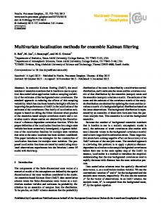
FIG. 1. WEF method with (a) N 5 100 and (b) N 5 10 4 . Data are shown as circles, the WEF as solid lines, and the optimal solution as dashed lines.
erences therein]. In this approach, a ‘‘Kalman gain matrix’’ is calculated from ensemble-average statistics at measurement times and employed to make a linear interpolation between current ensemble states x n (t 2m ) and error-contaminated measurements. These generate a new ensemble of realizations x n (t 1m ) for n 5 1, . . . , N, constructed each time measurements are taken. This is traditionally called the ‘‘analysis step’’ in filtering applications. The new set of realizations are then evolved forward under the model dynamics to the next measurement time, and the procedure is repeated. Unfortunately, the EnKF prescription for generating the new samples x n (t 1m ), n 5 1, . . . , N does not, in general, produce an ensemble representative of the correct conditional distribution (1). Only for linear dynamics with Gaussian error statistics does the interpolation scheme with the Kalman gain matrix lead to such a correct ensemble. The EnKF analysis step lacks any fundamental justification for nonlinear dynamics with non-Gaussian statistics.
m 5 1, . . . , M, where r m are random observation errors. For the case where the latter are assumed independent and normally distributed, Miller et al. (1999) have calculated the exact conditional statistics from the forward Kolmogorov equation and Bayes’s rule. They found that the EnKF lags in tracking the transition from one well to the other in this model compared with the optimal filter result (see also Eyink et al. 2002b). Evensen and van Leeuwen (2000) acknowledged this problem with the EnKF and further found that the inability of the EnKF to track transitions accurately is rooted in the linear analysis at measurement times. We study in this same model some alternative ensemble methods of data assimilation with a different analysis step than the EnKF. As will be shown later, these new methods successfully track the state transitions for Eq. (2). In what follows it will also be clear that these methods have important appealing characteristics: they are very simple, efficient, and potentially applicable to large-scale spatially extended systems. 2. Bayesian ensemble methods The idea behind each of these methods is just to apply Bayes’s rule (1) at measurement times t m appropriately. Suppose that an F-dimensional vector h m (x) is measured at time t m , where h m is an arbitrary function of the Ddimensional state vector x. The outcome of the measurement will be assumed to be of the form
2588
MONTHLY WEATHER REVIEW
y m 5 h m [x(t m )] 1 r m , where r m is a normally distributed observation error with mean zero and covariance matrix R m . Then Bayes’s rule (1) at the measurement time t m becomes P(x, t 1m )
5
5
1 exp 2 [y m 2 h m (x)] T R21 m [y m 2 h m (x)] 2 Nm
6
P(x, t 2m ), (3)
where we abbreviate, for simplicity, P(x, t) 5 P[x, t | R (t)]. We now investigate several schemes for implement-
w n (t 1m ) 5
Nm
O w (t)M [x (t)]. n
a. Weighted ensemble filter The first method that we study is referred to here as the weighted ensemble filter (WEF); in the applied probability literature it is more commonly referred to as a ‘‘particle filter.’’ It was originally proposed by Ulam and von Neumann (1949) but only became more widely known after the work of Enachescu (1985). In this approach, one assigns to each sample x n (t) a variable weight w n (t), n 5 1, . . . , N, which is altered according to (3) at measurement times. Each of the realizations is given initial weight 1/N at the starting time. At a measurement time t m , Bayes’s rule is applied to recalculate the weight for each realization as
1
N
^M(t)& 5
ing this formula when using ensemble methods to evolve the statistics of a dynamical system.
1 2 exp 2 {y m 2 h m [x n (t 2m )]}T R21 m {y m 2 h m [x n (t m )]} 2
where N m is a normalization factor to ensure that S Nn51 w n (t) 5 1 for all times t. Weights remain constant between measurement times. In this scheme, averages of a moment variable M(x) over the weighted ensemble are given by n
n51
Note that the calculation of the weights is very simple, even when x has very high dimension D. The most expensive operation, in fact, is the evaluation of the nonlinear function, h m (x), N times. This scheme can be shown to be convergent to the optimal filter estimate in the limit as N → ` [see Del Moral (1996) and also the useful, recent review of Crisan and Doucet (2002)]. However, the rate of convergence is rather slow, with the O(1/ÏN) errors typical of all Monte Carlo methods. Furthermore, in practical applications, an operational ensemble prediction can deal with only moderate values of N, generally N K 100 [for a discussion of this point see Miller and Ehret (2002), where extensive further references to the literature may be found]. For these reasons, the convergence properties of the scheme as N → ` may be mostly of academic interest. Instead, one must consider the performance of the method with only a moderate number of samples. Therefore, in our test of this method and the other methods introduced below, we consider both a large ensemble, with N 5 10 4 , and a smaller one, with N 5 100, to see the effect of a reduced number of samples.
VOLUME 131
2
w n (t 2m ),
Results from the WEF method in the model system (2) are shown in Fig. 1, with N 5 100 samples used in obtaining Fig. 1a and N 5 10 4 in obtaining Fig. 1b. The simulated measurements are represented by the open circles. These were generated by adding independent normal random errors of zero mean and standard deviation 0.2 to a particular solution x(t) of (2), sampled at unit time intervals. The solution considered experienced a state transition from x 5 11 to x 5 21 sometime around t 5 4;5. For reference, we have plotted in dashed lines the optimal filter mean and plus and minus the standard deviation, which were all calculated using the forward Kolmogorov equation, as in Miller et al. (1999). As can be seen, the optimal filter estimate clearly indicates the transition around t 5 4;5. The WEF estimates of the same statistics are represented by solid lines in Fig. 1. As shown in Fig. 1b, the WEF method for N 5 10 4 also succeeds in tracking the transition at t 5 4;5, whereas in Miller et al. (1999) and Eyink et al. (2002b), it was shown that the EnKF lags by one time unit in making the transition. Evensen and van Leeuwen (2000) have traced this defect of the EnKF to the linear analysis, using the Kalman gain matrix. We see here that an ensemble method that employs an analysis scheme based instead on an approximate implementation of Bayes’s theorem correctly tracks the transition with no lag. The WEF result for N 5 10 4 is, in fact, quite close to the optimal filter result, except that after the transition the fluctuation effects in the averages are rather large. Most of the weight is given then to just a few samples that
NOVEMBER 2003
KIM ET AL.
2589
made the transition from x 5 1 to x 5 21 at the correct time. Therefore, the effective size of the ensemble is much less than 10 4 and only a few fluctuating samples dominate the averages. Nevertheless, the correspondence of the WEF for N 5 10 4 with the optimal filter averages is quite acceptable. However, for N 5 100, the agreement is much worse. As seen in Fig. 1a, the transition is now missed entirely, even after three consecutive measurements in the well at x 5 21. The only sign of the transition is a broadening of the variance after the third measurement. The reason is that, with only 100 realizations, no sample made the transition from x 5 1 to x 5 21 at the correct time (or even after the subsequent three measurements). Therefore, the transition to x 5 21 occurred only very slowly because of the gradual growth of the weights, after successive measurements, of samples already residing in the x 5 21 well. From this example we see that the consequences of small sample size in the WEF method may be severe for realistic applications, where N is at most a few hundreds. b. Weight resampling filter One idea to overcome the problem with effective reduced sample size in the WEF method is to redistribute the large weights. This leads us to a simple modification of WEF, already considered in other contexts by several authors (see Kitagawa and Gersch (1996); Kitagawa 1996, 1998; Gordon et al. 1993), which we call here the weight resampling filter (WRF). Its potential application to data assimilation for atmospheric predictability has already been studied by Anderson and Anderson (1999) and Pham (2001) in the context of the chaotic three-dimensional model of Lorenz (1963). This method is almost the same as that of the WEF save for an additional resampling at measurement times. That is, after we have new weights w n (t 1m ) the same as in the WEF method above, we select a new N-sample ensemble of realizations, each with the same weight 1/N. The new ensemble is generated by selecting from the N values x n (t 2m ), n 5 1, . . . N of the old ensemble, with probabilities determined by the weights w n (t 1m ). After this resampling, some of the realizations may disappear, and some of them may be replicated several times. The result, however, is that large weights are redistributed over samples of equal weight. Note that for deterministic dynamics, replicated samples will evolve in unison in the future and, hence, shall effectively represent still a single sample with a large weight. This is not a problem in our stochastic system (2), or in other systems with random model error, because identical initial conditions that experience different realizations of the system noise have distinct future evolutions. However, for deterministic dynamics, the replicated samples in the WRF method must be variously perturbed to show different future behaviors. Such perturbations may be generated by the singular vector or bred vector methods discussed in
FIG. 2. WRF method with (a) N 5 100 and (b) N 5 10 4 . Data are shown as circles, the WRF as solid lines, and the optimal solution as dashed lines.
Miller and Ehret (2002), by density kernel methods, discussed in Hu¨rzeler and Ku¨nsch (1998), Anderson and Anderson (1999), and Pham (2001), or by an effective combination of these. In Fig. 2, we plot the results of our experiment with the WRF estimator in the model system (2) for N 5 100 and for N 5 10 4 . Notations are the same as in Fig. 1. Just as in the WEF method, the WRF scheme produces an estimate that converges to the optimal filter estimate as N → ` (see Crisan and Doucet 2002). Indeed, in Fig. 2b we see that the WRF with N 5 10 4 is nearly indistinguishable from the optimal filter for the statistics considered. As expected, the result is better than that of the WEF with the same number of samples and, in particular, the fluctuations due to small effective sample size are reduced. Furthermore, the WRF estimate for N 5 100, shown in Fig. 2a, now succeeds in tracking the transition, where the WEF failed to do so at all. However, there is still a lag, just as in the EnKF. The reason for this is easy to understand. Since a sequence
2590
MONTHLY WEATHER REVIEW
of accurate measurements was taken at times t 5 1 to 3 in the well at x 5 11, all realizations ‘‘died out’’ in the other well at x 5 21. That is, those realizations acquired small weights under Bayes’s rule (1) and, consequently, were selected to survive with small probability upon resampling. After several such resamplings, the entire population of N 5 100 samples resided in the well at x 5 11. Then, despite the measurements indicating a transition at t 5 4;5, there were simply no ensemble members in the opposite well at x 5 21 to receive the higher weights under the Bayes’s rule calculation. Consequently the WRF method required a few of the samples in the well at x 5 11 to dynamically make the transition to the opposite side, and this required additional time. The time was shorter than with the WEF because the samples most likely to make the transition were preferentially resampled. As soon as a few samples moved to the 21 well, they received most of the weight at the next measurement and then repopulated that well. However, in making the transition, a lag time still resulted. This type of problem is likely to be generic when the WRF method is applied for moderate sample size N to nonlinear systems with multimodal statistics. c. Parametric resampling filter It is desirable to have a resampling method that can keep uniform weights, as does the WRF, but avoids the difficulty of the complete disappearance of realizations with small weights. A solution is to parametrically model the probability density so that small probability events are preserved, even for small values of N. In other words, the idea is to employ a parametric density function P(x; l) to approximate the real probability density function at measurement times t m . We outline here a particular example of such a method, which we call the parametric resampling filter (PRF), that uses an exponential family of probability density functions (pdfs). Full details of the method are outlined here in the appendix. In this section we simply describe the method in its application to the model equation (2). A convenient form for the parametric representation of the pdf in this case is P(x; l) 5 exp(l1 x 1 l 2 x 2 ) · Q(x), where l 5 (l1 , l 2 ). Chosen here to be an equally weighted mixture of two Gaussians, Q(x) is an appropriate reference pdf: Q(x) 5
5
[
1 1 1 exp 2 2 (x 1 1) 2 2 Ï2ps 2 2s 1
1 Ï2ps 2
[
exp 2
]
VOLUME 131
Eyink et al. (2002a,b,c) use such a representation to carry out data assimilation for the model by moment closure methods. In principle, convergence to the exact pdfs can be obtained by taking more Gaussians in the weighted sum for Q(x), approaching the invariant measure P s (x). The basic idea is then (i) to fit such a distribution P(x; l 2m ) to the empirical ensemble of samples x n (t 2m ), n 5 1, . . . , N before the measurement, (ii) to apply Bayes’s rule to generate a new parametric model distribution P(x; l 1m ) subsequent to the measurement, and (iii) to sample this distribution to generate a new ensemble of samples x n (t 1m ), n 5 1, . . . N after the measurement. Step (i) is achieved by determining the moments m i 5 ^x i &, i 5 1, 2 empirically from the N-sample ensemble
m i (t 2m ) 5
1 N
O [x (t )] , N
2 m
n
To fit the statistics by the parametric model, we must determine corresponding values of l1 , l 2. This is accomplished by carrying out the following maximization:
l2m 5 argmax {lT m2m 2 F(l)}, l
where m 2m 5 [m1 (t 2m ), m 2 (t 2m )], and F(l) is the cumulant generating function F(l) 5 ln[# exp(l1 x 1 l 2 x 2 )Q(x) dx] given explicitly below. Step (ii) is carried out simply by setting l1 (t 1m ) 5 l1 (t 2m ) 1 y m /R m , l 2 (t m1) 5 l 2 (t 2m ) 2 1/(2R m ), because of the exponential form of the parametric representation. Step (iii) is made simpler by completing squares in the parametric model to write P(x; l) 5
1 Ï2ps 2 (l)
1
5
3 w2 (l) exp 2
5
6
1 [x 2 j2 (l)] 2 2s 2 (l)
1 w1 (l) exp 2
]6
where s 2 5 k 2 /16. This already gives a reasonable representation of the bimodal conditional pdfs of the model.
62
1 [x 2 j1 (l)] 2 2s 2 (l)
,
(4) where w 6 (l), j6 (l), and s (l) are elementary functions of the parameters l: w6 (l) 5
e6l1 s 2(l)/s 2 , 2 cosh[l1 s 2 (l)/s 2 ]
1
j6 (l) 5 s 2 (l) l1 6
1 (x 2 1) 2 . 2s 2
i 5 1, 2.
i
n51
s 2 (l) 5
2
1 , s2
and
s2 . 1 2 2l 2 s 2
The convex ‘‘free energy’’ F(l) is found from the same calculation to be
NOVEMBER 2003
2591
KIM ET AL.
metric pdf for N 5 100 and N 5 10 4 . As for the WRF method, fluctuations are reduced by the resampling, relative to the WEF statistics at the same value of N. The results are not as good as those for the WRF in the large ensemble with N 5 10 4 , but they could be improved by a parametric model with a mixture of more than two Gaussians. Even for the double-Gaussian pdf, the agreement is quite satisfactory. Furthermore, for N 5 100 the results are the best of all the approximation methods considered, successfully tracking the transition, with relatively small fluctuations. The key to success in following the measurements without a time lag is the presence of both Gaussians in the model, even when the weights w6 (l) of one or the other become small. As soon as measurements indicate a transition back to that side, Bayes’s rule makes the corresponding weight large, and resampling repopulates that well with many samples. Note in this one-dimensional model that EOFs, singular vectors (SVs), bred vectors, etc. all coincide, and that simply generating samples in the wrong well by a superposition of ‘‘optimal growth’’ modes would not solve the problem. In that case, as for the WRF, there would be a time lag in tracking the transition, required for some samples to make the excursion to the correct well on the opposite side. There is an additional advantage of the PRF method, involving the quantity called relative entropy of a probability density P. With respect to the longtime ‘‘climate state’’ P s , relative entropy is defined by H(P | Ps ) 5
FIG. 3. PRF method with (a) N 5 100 and (b) N 5 10 . Data are shown as circles, the PRF as solid lines, and the optimal solution as dashed lines. 4
F(l) 5
[ ]
s 2 (l) 2 2 s (l) (s l1 1 2l 2 ) 1 ln 2 2s s 1 ln cosh
[ ]
l1 s 2 (l) . s2
Now the N samples can be generated for n 5 1, . . . , N by first making a random selection of one of the Gaussians with probabilities w6 (l) and then, for the 6 term selected, taking x n 5 j6 (l) 1 s (l)n n . Here n n , n 5 1, . . . , N is a sequence of independent, normally distributed random variables with mean 0 and variance 1. These formulas all have relatively simple generalizations to multidimensional systems, when the reference pdf is taken to be a weighted sum of Gaussians. See the appendix for those formulas and computational details in the general case. In Fig. 3 we plot the results of the PRF method for our model system (2), with the double-Gaussian para-
E
dx P(x) ln
[ ] P(x) Ps (x)
(5)
(e.g., see Kleeman 2002). Consider the entropy of a time sequence of PDFs P(t) obtained by exactly solving the filtering problem for measurements at a discrete set of times t m , m 5 1, . . . , M. Assuming climate statistics hold initially, then H(t) 5 0 at t 5 0, and it does not change until there is a difference of P(t) from P s due to information acquired from observations. When a measurement occurs, there is an upward jump in entropy whose size is a numerical measure of the information gain from, or ‘‘utility’’ of, the observations (see Kleeman 2002). Between measurements, H(t) decreases back to zero because the pdf’s P(t) at large t . 0 converge again to P s . This is an exact H theorem for Markov stochastic processes like our model (2). Parametric models give an approximation to the entropy, as H[P˜(t) | P˜ s ], where P˜(t) 5 P[l(t)] and P˜ s 5 P(l s ). Here, the parameters l s should be chosen so that moments of P(l s ) match those of the exact P s . It is straightforward to show that for exponential families of parametric pdfs, as considered in the PRF method, ˜ | P˜ s ] 5 [l (t) 2 l s ]T m (t) 2 {F [l (t)] 2 F(l s )}. H [P(t) ˜ (t) in Hence, it is easy to calculate this approximation H the PRF method, along with statistics such as the conditional mean and variance.
2592
MONTHLY WEATHER REVIEW
VOLUME 131
FIG. 4. Relative entropy for (a) the optimal solution, and computed from the PRF method outcome with (b) N 5 100 and (c) N 5 10 4 .
In Fig. 4 we show results for the relative entropy in our model (2). Fig. 4a depicts the exact entropy H(t) calculated by formula (5), using the optimal filter PDF’s P(t) from the forward Kolmogorov equation and Bayes’s rule. We see that there is a large information gain from the measurement at time t 5 4, with a rapid loss immediately thereafter. In fact, if there were no subsequent measurements, then the entropy would drop close to zero by about time t 5 6. Thus, with just one measurement indicating a transition from 11 to 21, one would lose predictability very quickly. However, with the additional measurements at times t 5 5, 6, 7 indicating continuing residence in the 21 well, a different behavior is observed. In this case, there is a very slow relaxation back to zero at long times after the last measurement at time t 5 7. The value of those final measurements is high, and the loss of prediction utility is very slow afterward. Figures 4b and 4c show the ap˜ (t) calculated from the PRF method, proximate entropy H with N 5 100 and N 5 10 4 in Figs. 4b and 4c, respec-
tively. They are quite similar to each other, except that the N 5 100 result is rougher, as expected. Their magnitudes are also similar to the true entropy H(t), although not exactly equal numerically. Most importantly, we see ˜ (t) captures the large gain of information at time that H t 5 4, followed by a rapid loss and the slow decay at long times after the last measurement at time t 5 7. These results indicate that the PRF method, even for moderate values of N, may yield a useful approximation to the relative entropy in cases where the statistics are far from Gaussian. 3. Conclusions and remarks In this paper we have discussed three ensemble filtering schemes, the weighted ensemble filter (WEF), the weight resampling filter (WRF), and the parametric resampling filter (PRF). The latter, in particular, appears to be new. They differ from the well-known ensemble Kalman filter (EnKF) in that the analysis step at the
NOVEMBER 2003
2593
KIM ET AL.
measurement times is carried out by an approximate implementation of Bayes’s theorem, not by a linear interpolation via a Kalman gain matrix. For a large enough number of samples, the Bayesian ensemble methods can all successfully track transitions in multimodal systems, where the EnKF performs less well. For smaller numbers of samples, the PRF performs the best of all the Bayesian methods in a simple test problem with bimodal statistics. This is an important consideration in practical applications since the number of samples that can be employed at operational forecast centers is restricted. The PRF method also provides a convenient approximation of relative entropy, which measures the information made available from observations on the system. All three of these Bayesian methods are potentially applicable to large-scale, spatially extended systems. In addition to filtering and prediction, it is possible to perform smoothing as well, using the same methods. Applied to a system with dynamics close to linear and statistics near-Gaussian, these new methods will yield results equivalent to those obtained with the ensemble Kalman filter. They should be most useful when applied instead to geophysical systems with multiple attractors and multimodal statistics, or with otherwise highly non-Gaussian distributions. Miller and Ehret (2002) give many examples of geophysical systems with multimodal statistical distributions, for instance, the Kuroshio Current south of Japan. Other examples, such as the El Nin˜o– Southern Oscillation (see Burgers and Stephenson 1999), may have unimodal statistics but still exhibit other symptoms of non-Gaussianity, such as nonzero skewness or kurtosis. Nonnormal distributions are to be expected for the nonlinear dynamical systems that govern most geophysical systems. Therefore, we believe that there will be important applications of the methods developed here to prediction of atmospheric and oceanographic systems. Acknowledgments. This work was carried out in part at Los Alamos National Laboratory under the auspices of the Department of Energy and supported by LDRDER 2000047. We also received support from NSF/ITR Grant DMS-0113649 (SK, GLE, and JMR), as well as from NASA Goddard Space Flight Center Grant NAG511163 (JMR). APPENDIX A Parametric Resampling Method In this appendix we briefly outline the parametric resampling method in the general case. Complete details will appear in a forthcoming article (G. L. Eyink and S. Kim 2003, unpublished manuscript, hereafter EyKi). The method is based upon modeling the system statistics by an exponential family of PDFs: P(x, t m ; l) 5 exp[l1T h m (x) 1 hTm (x)l 2 h m (x)] · Q(x), where h m (x) is the measured F vector at time t m , and
l 5 (l1 , l 2 ), where l1 is an F vector, and l 2 is a symmetric F 3 F matrix. An appropriate reference PDF, Q(x), may be chosen, for example, to be a weighted sum of Gaussians. Most of the method does not depend upon any particular choice of Q(x). As discussed in section 2c, the analysis at the measurement times t m , m 5 1, . . . , M is carried out in three steps. • Step (i). In order to determine l 2m , we choose P(x; l) to match the empirical ensemble x n (t 2m ), n 5 1, . . . , N for the average of a moment vector M 5 (M1 , M 2 ):
E
dx M(x)P(x; l2m ) 5
1 N
O M[x (t )], N
n
2 m
n51
where M1 (x) 5 h m (x), and M 2 (x) 5 h m (x)hTm(x). Given the value on the rhs—call it m 2m —we can determine the corresponding value l 2m by the maximization
l2m 5 argmax {lT m2m 2 F(l)},
(A1)
l
where F(l) 5 ln{# dx exp[lTM(x)]Q(x)}, and lTm 5 l1 · m1 1 l 2 : m 2 . • Step (ii). After choosing l 2 , we apply Bayes’s rule to get the updated l 1 5 (l11, l 12 ), namely,
l11 5 l21 1 R21 y
1 l12 5 l22 2 R21 . 2
• Step (iii). Draw N independent samples x n (t 1m ), n 5 1, . . . N from the new distribution P(x; l 1m ). This is the only step that depends upon a particular choice for the reference pdf. Various possibilities are discussed in a forthcoming article (EyKi). The simplest case arises when the measured variables are linear in the state vector: h m (x) 5 d m 1 H mx, where d m is an F vector, and H m is an F 3 D matrix. It is then very convenient to take Q as a sum of Gaussians:
Ow
[
Q(x) 5
s51
]
1 exp 2 C21 s : (x 2 j s )(x 2 j s ) 2
S
s
Ï(2p) D det(C s )
,
where S Ss51 w s 5 1, and j s , C s are the mean and covariance, respectively, of the sth Gaussian. The terms in the sum should be selected so that Q(x) is a reasonable approximation to the steady-state measure P s (x), at least in applications to climate forecasting. Such a representation can be obtained empirically from conditional averaging over a long time series of the dynamics, given some identified set of ‘‘statistical states’’ or ‘‘regimes’’ s 5 1, . . . , S of the system. Otherwise, for more short-range forecasting, the reference PDF should be chosen as Q(x, t) to be explicitly time dependent and to reflect the phase-space divergence of sample solutions on those time scales. We do not further consider that problem here.
2594
MONTHLY WEATHER REVIEW
To resample from the PDF after conditioning upon measurements, we note that (4) can be generalized, under our stated assumptions, to P(x; l) 1 exp 2 C21 s (l) : [x 2 j s (l)][x 2 j s (l)] S 2 5 ws (l) , s51 Ï(2p) D det[C s (l)] where w s (l), j s (l), and C s (l) will be given explicitly in EyKi. The N samples can be generated, for example, by first making a random selection of one of the Gaussians with probabilities w s (l) and then, for the ‘‘regime’’ s n selected, taking
O
5
6
On D
x n 5 j sn (l) 1
n,d
s sn , d (l)e sn , d (l)
d51
for n 5 1, . . . , N. Here s2s,d(l) are the eigenvalues of Cs(l), and es,d (l) are the corresponding eigenvectors for s 5 1, . . . , S, d 5 1, . . . , D, and nn,d , n 5 1, . . . , N, d 5 1, . . . , D is a sequence of independent, normally distributed random variables with mean 0 and variance 1. In general, the resampling step (iii) is the most computationally intensive part of the analysis. Carried out as above, it requires diagonalizing the D 3 D matrices C s (l) for any required l. This will be too expensive to carry out in general. Instead, the forthcoming article (EyKi) will detail alternative procedures based upon Monte Carlo–Markov chain sampling methods, which require only diagonalizing the fixed set of l-independent matrices C s , s 5 1, . . . , S. The corresponding eigenvectors e s,d , s 5 1, . . . , S, d 5 1, . . . , D are the conditional empirical orthogonal functions (CEOFs) of the system, corresponding to each of its ‘‘statistical states’’ or ‘‘regimes.’’ Alternatively, knowing C s , the corresponding SVs may be constructed by the procedure discussed in Ehrendorfer and Tribbia (1997) (see also Miller and Ehret 2002). For small sample sizes N, the generated ensemble may better represent the pdf a finite time later if the expansion is given in terms of SVs rather than EOFs. Except for step (iii) the entire procedure is carried out in a space of lower dimension than D. The minimization in step (i) is over F 1 F(F 1 1)/2 5 F(F 1 3)/2 parameters. The Bayesian update in step (ii) and the calculation of w s (l), j s (l), and C s (l) in step (iii) are accomplished by linear algebra operations in the space of dimension F. Of course, these steps may also be nontrivial when the number of measurements F is large. REFERENCES Anderson, J. L., and S. L. Anderson, 1999: A Monte Carlo implementation of the nonlinear filtering problem to produce ensemble assimilations and forecasts. Mon. Wea. Rev., 127, 2741–2758.
VOLUME 131
Burgers, G., and D. B. Stephenson, 1999: The ‘‘normality’’ of El Nin˜o. Geophys. Res. Lett., 26, 1027–1030. Crisan, D., and A. Doucet, 2002: A survey of convergence results on particle filtering methods for practitioners. IEEE Trans. Signal Process., 50, 736–746. Del Moral, P., 1996: Nonlinear filtering using random particles. Theor. Probab. Appl., 40, 690–701. Ehrendorfer, M., and J. J. Tribbia, 1997: Optimal prediction of forecast error covariances through singular vectors. J. Atmos. Sci., 54, 286–313. Enachescu, D. M., 1985: Monte Carlo method for nonlinear filtering. Proceedings of the Fourth Pannonian Symposium on Mathematical Statistics, Mathematical Statistics and Its Applications, Kluwer. Evensen, G., 1994: Sequential data assimilation with a nonlinear quasi-geostrophic model using Monte Carlo methods to forecast error statistics. J. Geophys. Res., 99 (C5), 10 143–10 162. ——, and P. J. van Leeuwen, 2000: An ensemble Kalman smoother for nonlinear dynamics. Mon. Wea. Rev., 128, 1852–1867. Eyink, G. L., J. M. Restrepo, and F. J. Alexander, cited 2002a: Algorithms for the practical implementation of a statistical–mechanical approach to data assimilation. [Available online at http://www.physics. arizona.edu/;restrepo/myweb/downloads/DOUB31-rev.ps.gz.] ——, ——, and ——, cited 2002b: A statistical–mechanical approach to data assimilation for nonlinear dynamics. II. Evolution approximations. [Available online at http://www.physics.arizona. edu/;restrepo/myweb/downloads/DOUB32-rev.ps.gz.] ——, ——, and ——, cited 2002c: A mean-field approximation in data assimilation for nonlinear dynamics. [Available online at http://www.physics.arizona.edu/;restrepo/myweb/ downloads/DOUB33-rev.ps.gz.] Gordon, N. J., D. J. Salmond, and A. F. M. Smith, 1993: Novel approach to nonlinear/non-Gaussian Bayesian state estimation. IEE Proc., 140F, 107–113. Hu¨rzeler, M., and H. R. Ku¨nsch, 1998: Monte Carlo approximations for general state space models. J. Comput. Graphic. Stat., 7, 175–193. Kitagawa, G., 1996: Monte-Carlo filter and smoother for non-Gaussian nonlinear state space models. J. Comput. Graphic. Stat., 5, 1–25. ——, 1998: A self-organizing state-space model. J. Amer. Stat. Assoc., 93, 1203–1215. ——, and W. Gersch, 1996: Smoothness Priors Analysis of Time Series. Lecture Notes in Statistics, Vol. 116, Springer-Verlag, 261 pp. Kleeman, R., 2002: Measuring dynamical prediction utility using relative entropy. J. Atmos. Sci., 59, 2057–2072. Kushner, H. J., 1962: On the differential equations satisfied by conditional probability densities of Markov processes, with applications. J. SIAM Control, 2A, 106–119. Lorenc, A. C., and O. Hammon, 1988: Objective quality control of observations using Bayesian methods: Theory, and a practical implementation. Quart. J. Roy. Meteor. Soc., 114, 515–543. Lorenz, E. N., 1963: Deterministic nonperiodic flow. J. Atmos. Sci., 20, 130–141. Miller, R. N., and L. L. Ehret, 2002: Ensemble generation for models of multimodal systems. Mon. Wea. Rev., 130, 2313–2333. ——, E. F. Carter Jr., and S. T. Blue, 1999: Data assimilation into nonlinear stochastic models. Tellus, 51A, 167–194. Pham, D. T., 2001: Stochastic methods for sequential data assimilation in strongly nonlinear systems. Mon. Wea. Rev., 129, 1194–1207. Stratonovich, R. L., 1960: Conditional Markov processes. Theor. Probab. Appl., 5, 156–178. Ulam, S., and J. von Neumann, 1949: The Monte Carlo method. J. Amer. Stat. Assoc., 44, 335–341.