Ensemble learning with trees and rules: Supervised, semi ... - IOS Press

Intelligent Data Analysis 18 (2014) 857–872 DOI 10.3233/IDA-140672 IOS Press

857

Ensemble learning with trees and rules: Supervised, semi-supervised, unsupervised Deniz Akdemira,∗ and Jean-Luc Janninkb a Plant

Breeding and Genetics, Cornell University, Ithaca, NY, USA Cornell University, Ithaca, NY, USA

b USDA-ARS,

Abstract. In this article, we propose several new approaches for post processing a large ensemble of conjunctive rules for supervised, semi-supervised and unsupervised learning problems. We show with various examples that for high dimensional regression problems the models constructed by post processing the rules with partial least squares regression have significantly better prediction performance than the ones produced by the random forest or the rulefit algorithms which use equal weights or weights estimated from lasso regression. When rule ensembles are used for semi-supervised and unsupervised learning, the internal and external measures of cluster validity point to high quality groupings. Keywords: Decision trees, ensemble learning, rule ensembles, semi-supervised learning, clustering

1. Review of ensemble methods Ensemble learning [22,25,28] provides solutions to complex statistical prediction problems by simultaneously using a number of models. By bounding false idealizations, focusing on regularities and stable common behavior, ensemble modeling approaches provide solutions that as a whole outperform the single models. Some influential early works in ensemble learning were by Breiman with Bagging (bootstrap aggregating) [2], and Freund and Shapire with AdaBoost [15]. These methods involve “random” sampling the “space of models” to produce an ensemble of base learners and a “post-processing” of these to construct a final prediction model [33]. In this article, we review several approaches for ensemble post-processing and propose some new ones. To this end, we summarize the ensemble generation procedure and post-processing procedure of [17]. The novel approaches tried here include post-processing rules and trees with partial least squares regression, weighing trees with their out-of-bag performances and truncation and kernel smoothing in the case of regression; a unsupervised and a semi-supervised clustering algorithm based on rules; rule based unsupervised and semi-supervised kernel matrix learning. Our illustrations indicate that these new models are competitive, if not superior, to some popular approaches. However, a main theme in this article is that the base learners and rules can be used as input variables in any learning problem and, in essence, tree and rule ensembles can be treated as features extracted from the original data. Our work can be considered as an extension of the methods in [17] and these are briefly summarized below. ∗ Corresponding author: Deniz Akdemir, Plant Breeding and Genetics, Cornell University, Ithaca, NY, USA. E-mail: da346@ cornell.edu.

c 2014 – IOS Press and the authors. All rights reserved 1088-467X/14/$27.50  This article is published online with Open Access and distributed under the terms of the Creative Commons Attribution NonCommercial License.

858

D. Akdemir and Jean-Luc Jannink / Ensemble learning with trees and rules

Some other recent literature that is parallel with the approaches taken in this paper include the ENDER algorithm [9], ensemble classification using generalized additive models [8], ensemble selection from libraries of models [6], weighting individual outputs in multiple classifier systems [36], subspace ensembles using neighborhood accuracy [37]. The ensemble clustering problem was recently introduced by Strehl and Ghosh [34]. The problem has attracted a fair amount of attention and a number of interesting techniques have been proposed [12,19,29]. Reviews of semi-supervised learning is available in [42] and [20]. In the remainder of this section, we will review the recently proposed importance sampling learning ensembles (ISLE) framework [17] for ensemble model-rule generation and post-processing. In Section 2, we propose some new ensemble post processing methods for supervised learning including partial least squares regression, multivariate kernel smoothing and use of out-of-bag observations. Rule ensemble approach to supervised learning is adapted to the unsupervised and semi-supervised clustering problem in Section 3. Section 4 is reserved for examples and simulations by which we compare the methods proposed here with the existing ones. Some remarks about hyper parameter choice and directions for future research are provided in Section 5. 1.1. ISLE approach Given a learning task and a relevant data set, we can generate an ensemble of models from a predetermined model family. Bagging bootstraps the training data set [2] and produces a model for each bootstrap sample. Random forest [5,24] creates models by randomly selecting a few aspects of the data set while generating each model. AdaBoost [15] and ARCing [4] iteratively build models by varying case weights and employ the weighted sum of the estimates of the sequence of models. There have been attempts to unify these ensemble learning methods. One such framework is the ISLE due to Popescu & Friedman [17]. We are to produce a regression model to predict the continuous outcome variable y from p vector of input variables x and a model family F = {f (x, θ) : θ ∈ Θ} indexed by the parameter θ is given to generate M models. The final ensemble models considered by the ISLE framework have an additive form: M  F (x) = w0 + wj f (x, θj ) (1) j=1 M {f (x, θj )}j=1 are

where base learners selected from F . ISLE uses a two-step approach to produce F (x). The first step involves sampling the space of possible models to obtain {θj }M j=1 . The second step M proceeds with combining the base learners by choosing weights {wj }j=0 in Eq. (1). The pseudo code to produce M models {f (x, θj )}M j=1 under ISLE framework is given below: Algorithm 1: ISLE(M, ν, η ) F0 (x) = 0. for j ⎧ = 1 to M  ⎪ ( cj , θj ) = argmin i∈Sj (η) L(yi , Fj−1 (xi ) + cf (xi , θ)) ⎪ ⎪ ⎪ (c,θ) ⎨ do Tj (x) = f (x, θj ) ⎪ ⎪ ⎪ ⎪ ⎩F (x) = F (x) + ν  c T (x) j

return

j−1

({Tj (x)}M j=1

j j

and FM (x).)

D. Akdemir and Jean-Luc Jannink / Ensemble learning with trees and rules

859

Here, L(., .) is a loss function; Sj (η) is a subset of the indices {1, 2, . . . , n} chosen by a sampling scheme η, and 0  ν  1 is a memory parameter. The classic ensemble methods of Bagging, Random Forest, AdaBoost, and Gradient Boosting are special cases of ISLE ensemble model generation procedure [33]. In Bagging and Random Forests the 1 for j = 1, 2, . . . , M. Boosting weights in (1 are set to predetermined values, i.e. w0 = 0 and wj = M calculates these weights in a sequential fashion at each step by having positive memory ν, estimating cj and takes FM (x) as the final prediction model. Friedman and Popescu [17] recommend learning the weights {wj }M j=0 using lasso [39]. Let T = n M (Tj (xi ))i=1 m=1 be the n × M matrix of predictions for the n observations by the M models in an ensemble. The weights (w0 , w = {wm }M m=0 ) are obtained from ˆ = argmin(y − w0 1n − T w) (y − w0 1n − T w) + λ w w

M 

|wm |.

(2)

m=1

λ > 0 is the shrinkage operator, larger values of λ decreases the number of models included in the final prediction model. The final ensemble model is given by M 

Fˆ (x) = w ˆ0 +

w ˆm Tm (x).

(3)

m=1

1.2. Rule ensembles The base learners in the preceding sections of this article can be used with any regression model, however they are often used with regression trees. Each decision tree in the ensemble partitions the input space using the product of indicator functions of simple regions based on several input variables. A tree with K terminal nodes define a K partition of the input space where the membership to a specific node, say node k, can be determined by applying the conjunctive rule rk (x) =

p

I(xl ∈ slk ),

l=1

where I(.) is the indicator function, x = (x1 , x2 , . . . , xp ) are the input variables. The regions slk are intervals for a continuous variable and a subset of the possible values for a categorical variable. Let R = (rk (xi ))ni=1 K k=1 be the n × K matrix of rules for the n observations by the K rules in the ensemble. The rulefit algorithm of Friedman and Popescu [18] uses the weights (w0 , w = {wk }K k=0 ) that are estimated from 

ˆ = argmin(y − w0 1n − Rw) (y − w0 1n − Rw) + λ w w

K 

|wk |

(4)

k=1

in the final prediction model Fˆ (x) = w ˆ0 +

K  k=1

w ˆk rk (x).

(5)

860

D. Akdemir and Jean-Luc Jannink / Ensemble learning with trees and rules

2. Post processing ensembles revisited We can use the base learners or rules in an ensemble as input variables in any regression method. Since the number of models in an ensemble can easily exceed the number of individuals in the training sample (p  n), we prefer regression methods that can handle high dimensional input. A few such ensemble post-processing methods like partial least squares regression, multivariate kernel smoothing and weighting are proposed in this section. We will compare these approaches to the existing standards random forests and rulefit in the Section 4. 2.1. Partial least squares regression The models in an ensemble are all aligned with the response variable and therefore we should expect that they are correlated with each other. When this is the case variable selection methods like lasso do not work particularly well, especially with regard to the problem of model selection. Partial least squares regression (PLSR) is a technique which is suitable for high dimensional regression problems where the predictor variables exhibit multicollinearity. An additional advantage in using PLSR is that response variables can be multivariate. In PLSR the input matrix X is decomposed into orthogonal scores S and loadings L X = SL

and the outcome Y is regressed on the first few columns of the scores S using ordinary least squares. This leads to biased but low variance estimates of the regression coefficients in model 1. PLSR incorporates information on both input and output variables in the loadings. PLSR behaves as shrinkage method [16] where the amount of shrinkage is controlled by the number of loadings included. An obvious question is to find the number of loadings needed to obtain the best generalization for the prediction of new observations. This is, in general, achieved by evaluating the cross-validated performance of the different PLSR models. In our experience setting the discrete shrinkage parameter in PLSR is easier than setting the continuous sparsity parameter in lasso regression. The illustrations following section demonstrate the good performance of PLSR for post processing trees or rules. PLSR, as opposed to lasso, achieves shrinkage without forcing sparsity on the input variables. The coefficients of the tree ensemble model in 2 or the rule ensemble model in 4 can be used to evaluate importances of trees, rules and individual input variables [18]. For the tree ensembles the importance of the kth tree is evaluated as Ik = |w ˆk |std(Tk )

measures the importance of the trees or rules, here std(Tk ) denotes the standard deviation for the output of the kth tree over the individuals in the training sample. For the rule ensembles the importance of the kth rule is calculated similarly as

Ik = |w ˆk | sk (1 − sk ) n

r (x )

where sk = i=1 nk i is the support of rule k. The individual variable importances are calculated from sum of the importances of the trees or rules which contain that variable. The PLSR model is in the same additive form as in Eq. (1), therefore the estimated weights w ˆ1 , w ˆ2 , . . . , w ˆM in the model can be used to calculate tree rule or variable importances the same way they were calculated for the lasso post processing approach. A measure of importance for each variable can be obtained as the sum of the importances of rules that involve that variable.

D. Akdemir and Jean-Luc Jannink / Ensemble learning with trees and rules

861

2.2. Multivariate kernel smoothing We will concentrate on kernel smoothing using the Nadaraya-Watson estimator. For a detailed presentation of the kernel smoothing, we refer the reader to [38]. The Nadaraya-Watson estimator is a weighted sum of the observed responses y. Let the value of base learners (trees or rules) at an input point x be written in a M dimensional vector t(x). The final prediction model at input point x can be obtained as n Kh (t(xi ) − t(x))yi . F (x) = i=1 n i=1 Kh (t(xi ) − t(x)) The kernel function Kh (.) is a symmetric function that integrates to one, h > 0 is the smoothing parameter. In practice, the kernel function and the smoothing parameter are usually selected using the cross validated performances for a range of kernel functions and smoothing parameter values. 2.3. Weighting ensembles using out-of-bag observations As mentioned earlier, most of the important ensemble methods combine the base models using ˆ by minimizing weights. Both bagging and random forest algorithms use equal weighting. Estimating w 1 (y − T w) (y − T w) 2

subject to the constraint w  0 gives the Stacking approach of Wolpert [41] and Breiman [3]. In stacking final prediction model is given by  F (x) = T (x)w. Subspace ensembles (SENA) [37] uses the idea of local neighborhood accuracy to obtain the ensemble model weights for the classification problem. Below we propose a similar weighting scheme based on the generalization performance of individual models. The ensemble generation algorithms based on bootstrapping the observations builds the base learners from the observations in the bootstrap sample, and leaves us with the out-of-bag observations to evaluate the generalization performance of that particular learner. The following weighting scheme will down weight the base learners which have bad generalization performance. Let (yoob i , xoobi ) denote the ith out-of-bag observation from model l for i = 1, 2, . . . , nl,oob . We have M base learners {Tl (x)}M l=1 . We can use M nl,oob Kh (yoob i − Tl (xoobi ))Tl (x) F (x) = l=1 M i=1 nl,oob i=1 Kh (yoob i − Tl (xoobi )) l=1 as the prediction of the response at input value x. This involves keeping track of the out-of-bag performance each model in the ensemble and using the weights nl,oob Kh (yoob i − Tl (xoobi )) , wl = M i=1 nl,oob l=1 i=1 Kh (yoob i − Tl (xoobi )) l = 1, 2, . . . , M.

862

D. Akdemir and Jean-Luc Jannink / Ensemble learning with trees and rules

The value of h controls the smoothness of the model. For large values of this parameter the kernel method will assign approximately equal weights to the learners Tl , l = 1, 2, . . . , M and hence it is equivalent to random forest weighting. Smaller values of the parameter assigns higher weights to the models with small out of bag errors. We can choose h to minimize the cross-validated errors. In addition, it is sometimes beneficial to eliminate the models with lowest weights from the final ensemble. Note that, a modification of the above model allows us to localize the predictions by weighting models based on their out of bag performance in the close neighborhood of an input point, say xnew , in spirit of the model in [37]. An estimator of the response at input value xnew can be written as M nl,oob F (xnew ) =

Kh1 (yoob i − Tl (xoobi ))Kh2 (xoobi − xnew )Tl (xnew ) Mi=1 nl,oob i=1 Kh1 (yoob i − Tl (xoobi ))Kh2 (xoobi − xnew ) l=1

l=1

where Kh1 and Kh2 are two kernel functions indexed by the width parameters h1 and h2. 3. Rule ensemble clustering The main difference between the supervised learning and unsupervised learning is the existence of a target variable in the former. The sample partitioning approaches discussed in the previous section partition the sample space into clusters. Each rule defines a clustering of the sample space into two components which give a good segregation of the target variable. When we have many target variables we can randomly map them to the real line and when we are not provided with target variables, we can construct our target variables by randomly mapping the input variables in a similar fashion. Consequently, each of these derived target variables (“concepts”) can be used to extract several interesting rules and overall cluster rules are obtained from combining the rules for many target variables into an ensemble distance matrix. By making an analogy to ISLE algorithm reviewed in the previous section, we can boost the search of the space of ”concepts” by including a memory parameter. The details of this clustering procedure are described below. Let Y be the n × q matrix of observed target variables for which a good segregation is needed. Let X be the n × p matrix of observed input variables to the clustering algorithm. We name the following algorithm semi-supervised importance sampling clustering algorithm (SS-ISCA). Algorithm 1: SS-ISCA(X, Y, M, m, ν ) R1 : A random projection of Y for j ⎧ = 1 to M Generate m rules {l (x)}m ⎪ =1 to estimate Rj from X : ⎪ ⎪ ⎪ ⎪ ⎪ Sj (x) ⇐ {l (x)}m ⎪ =1 ⎨ j n do T (X) ⇐ {Sj (xi )}i=1 d=1 ⎪ ⎪ ⎪ ⎪ Rj+1 : A random projection of Y ⎪ ⎪ ⎪ ⎩ Rj+1 ⇐ (I − νPT (X) )Rj+1 return (T (X))

D. Akdemir and Jean-Luc Jannink / Ensemble learning with trees and rules

863

Here PT (X) is the projection matrix on to the space spanned by the columns of T (X) calculated as T (X)[T (X) T (X)]− T (X). In our implementations “a random projection” was interpreted as a random linear projection though this is not necessary. The projection step and a positive ν value allows the algorithm to cover the target space quicker. However when a nonzero memory parameter is used the computational burden grows quickly as the algorithm advances in its stages. One simple strategy is to apply lasso regression to select rules at each stage j and therefore reducing m. Another strategy is to sample the columns of T (X) to calculate PT (X) at each stage, and in this case ν is used as the sampling proportion. We have used both of these techniques successfully for high dimensional clustering problems. Of course, if the memory parameter ν is set to zero then we do not have to worry about calculating PT (X) . In this case the SS-ISCA algorithm is parallelizable. An implementation of SS-ISCA can be tried at the Triticeae Toolbox (T3). T3 is the web portal for the data generated by the Triticeae Coordinated Agricultural Project (CAP), funded by the National Institute for Food and Agriculture (NIFA) of the United States Department of Agriculture (USDA). T3 contains SNP, phenotypic, and pedigree data from wheat and barley germplasm in the Triticeae CAP. From T (X)n×r , a similarity matrix can be obtained as S(X) = T (X)T (X) /r. The ij th element of S(X) is the percentage of times the ith and the j th observations fire the same rules. From the similarity matrix S(X), we calculate a distance matrix D(X). The clustering of the observations is accomplished by applying a distance based hierarchical clustering algorithm [27] to the rule based distance matrix D(X). The method we have used to combine the clusters from many rules is referred to as the cluster based similarity partitioning in Ghosh et. al. [34]. Note that for a set of new observations Xnew , we can calculate T (Xnew ) without the knowledge of the corresponding target variables. In distance based hierarchical clustering, first, each object is assigned to its own cluster. At each consecutive stage the two most similar clusters are joined until there is a single cluster. The distances between clusters are recalculated at each stage by a linkage criterion such as single-linkage, complete linkage or average linkage. In our illustrations in the following section, we have uniformly used the average linkage criterion for combining clusters. A modification of the semi supervised clustering algorithm when the target variable is univariate takes advantage of the rule importances. To obtain M rules for the target variable y use the ISLE algorithm to extract rules and use either PLSR or lasso post-processing to estimate the weights w. ˆ a similarity matrix can be obtained as S(X) = T (X) From T (X)

and the estimated weights w ˆ s(1 − s))T (X) /r where s = (s1 , s2 , . . . , sr ) are the supports of rules 1 to r. diag(|w| For generation of rules useful for ensemble clustering when there are no target variables, we modify the semi-supervised rule generation algorithm in 1 as follows (importance sampling clustering algorithm): Algorithm 2: ISCA(X, M, m, ν ) R1 : A random projection of X for j ⎧ = 1 to M Generate m rules {l (x)}m ⎪ =1 to estimate Rj from X : ⎪ ⎪ ⎪ ⎪ ⎪ Sj (x) ⇐ {l (x)}m ⎪ =1 ⎪ ⎨ j n do T (X) ⇐ {Sj (xi )}i=1 d=1 ⎪ ⎪ ⎪ Rj+1 : A random projection of X ⎪ ⎪ ⎪ ⎪ ⎪ ⎩Rj+1 ⇐ (I − νPT (X) )Rj+1

return (T (X))

864

D. Akdemir and Jean-Luc Jannink / Ensemble learning with trees and rules

0.8

0.90

0.6

0.85

0.4 0.80

0.2 0.75

0.0 0.70

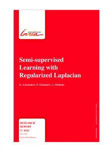
Fig. 1. 10 fold cross validated accuracies measured by correlation for the FHB data set. The ensemble of rules with PLSR has slightly higher accuracy compared to its alternative rules with lasso. The number of trees was set to 200. Maximum depth allowed for each tree or rule was set to 5.

kst

ksr

rf

wt(oob)

w(oob)

t(lasso)

r(lasso)

t(plsr)

r(plsr)

kst

ksr

rf

wt(oob)

w(oob)

t(lasso)

r(lasso)

t(plsr)

r(plsr)

−0.2

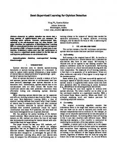
Fig. 2. The boxplots in Fig. 2 compare the different approaches to ensemble post processing for the scenario in Example 2. The number of trees generated was 200, maximum depth parameter was set to 2.

Hierarchical clustering produces nested clusterings of the data set. In order to determine the final clustering, the number of clusters has to be determined. When the clustering problem is accompanied by external class labels or external benchmarks and the number of clusters is known, the quality of a cluster can be measured by Rand measure (R) [30], Jaccard index (J) [10], Fowlkes Mallows index (FM) [13], Wallace indices (W01, W10), etc... Otherwise internal clustering quality measures like Silhouette (silhouette) [32], Dunn index (dunn) ( [11], Connectivity (connect) [7] can be used to identify the number of clusters. These measures can also be used to compare the quality of several clusterings. The article by Handl et al. [21] provides an excellent overview of cluster validation measures. Each rule gives a binary partition of the input space. Therefore, an ensemble of rules together can be seen as a multiple clustering of the input space. Multiple clustering approach argues that multiple sets of clusters provide more insight then only one solution. For instance, when grouping genes with similar function we need a multiple clustering approach since some genes might have multiple functional roles. Similarly, to gain insight about the history of species, we could use multiple clusterings of the individuals based on the marker data from different chromosomes. In a sense, multiple clusterings represent different views of grouping the data. ISCA and SS-ISCA algorithms can benefit from such a view and the author believes that these algorithms are flexible enough to answer such questions. 4. Case studies and experiments In this section we will deliver several data analysis that uses the supervised, semi-supervised and unsupervised approaches discussed in this paper. The main properties of the data sets that are used in this section are summarized in Table 1. The following ensemble models are compared in the context of supervised learning:

D. Akdemir and Jean-Luc Jannink / Ensemble learning with trees and rules

865

Table 1 Important characteristics of data sets used Data set FHB data Simulated data Friedman simulated data Boston housing data Fisher’s iris data Stem rust data Mouse microarray data

Individuals 622 150 1000 506 150 374 6

Input variables 2251 100 100 13 4 1624 147

Target variables FHB, DON (Continuous) Y (Continuous) Y (Continuous) Median house value (Continuous) Species (Categorical) Stem rust resistance (Continuous) NA.

Used in examples 4.1, 4.6, 4.9 4.2 4.3 4.4 4.5 4.7 4.8

1. r(pslr): Partial Least Squares Regression with Rules, 2. t(pslr): Partial Least Squares Regression with Trees, 3. r(lasso): lasso with Rules, 4. t(lasso): lasso with Trees, 5. w(oob): Weighting Using Out-of-Bag performance, 6. wt(oob): Weighting Using Out-of-Bag performance (best 60% of the trees), 7. rf: Random Forest, 8. ksr: Kernel Smoothing with Rules, 9. kst: Kernel Smoothing with Trees. In all these models, hyper parameters of the models are set using 10 fold cross validation in the training sample. Aggressive use of cross-validation can be supported by the theorem in [40]. The models 3, 4, and 7 are the existing methods and models 1, 2, 5, 6, 8, and 9 are the models introduced in this paper. Our first example involves the Fusarium head blight (FHB) data set that is available from the author upon request. A very detailed explanation of this data set is given in [26]. Example 1. (FHB Data, Regression) FHB is a plant disease caused by the fungus Fusarium Graminearum and results in tremendous losses by reducing grain yield and quality. In addition to the decrease in grain yield and quality, another damage due to FHB is the contamination of the crop with mycotoxins. Therefore, breeding for improved FHB resistance is an important breeding goal. Our aim is to build a prediction model for FHB resistance in barley based on available genetic variables. The FHB data set included FHB measurements along with 2251 single nucleotide polymorphisms (SNP) on 622 elite North American barley lines. The data set included the results of the experiment in 3 locations in years 2006, 2007, and 2008. We have used a semi-parametric mixed model (SPMM) to account for the location and year effects. The total genetic effects of each line is estimated by solving the mixed model equations and obtaining corresponding estimated best linear unbiased predictors for the random effects. Our SPMM for the n × 1 response vector y is expressed as y = Xβ + Zg + e

(6)

where X is the n × p design matrix for the fixed effects, β is a p × 1 vector of fixed effects coefficients (mean, location, year), Z is the n × q design matrix for the random effects (lines); the random effects (g  , e ) are assumed to follow a multivariate normal distribution with mean 0 and covariance  2 σg K 0 0 σe2 In  where K is a q × q similarity matrix obtained as K = M M  / diag(M M  ) and M is the 622 × 2251 dimensional markers matrix.

866

D. Akdemir and Jean-Luc Jannink / Ensemble learning with trees and rules

0.8

0.95

0.7

0.90 0.6

0.5

0.85 0.4

kst

ksr

rf

wt(oob)

w(oob)

t(lasso)

r(lasso)

t(plsr)

kst

ksr

rf

wt(oob)

w(oob)

t(lasso)

r(lasso)

t(plsr)

r(plsr)

Fig. 3. The boxplots in Fig. 2 compare the different approaches to ensemble post processing for the scenario in Example 3. Number of trees was set to 200, and the maximum depth parameter was set to 2.

r(plsr)

0.80

0.3

Fig. 4. 10 fold cross validated accuracies for the “Boston Housing” data are displayed by the boxplots. The PLSR approach has the best cross validated prediction performance. We have generated 300 trees by the ISLE approach and maximum depth parameter was set to 4. For the methods that use a kernel function we have uniformly used the Gaussian kernel. The sparsity parameters of the lasso or PLSR and the kernel width parameters were obtained by minimizing 10 fold cross validated errors in the training data.

In the second step the EBLUPS of genetic values of the 622 lines are estimated using models 1:10. The 10 fold cross validated accuracies measured by the correlations of true responses to the predicted values are displayed in Fig. 1. Example 2. (Simulated Data, Regression) In our second example we repeat the following experiment 100 times. Elements of the 150 × 100 input matrix X are independently generated from a uniform(0, 1) distribution. The elements of the coefficient matrix β were also generated independently from unif(0, 1) and 85% of these were selected randomly and set to zero. 150 dimensional response vector y was generated according to y = Xβ + e where e was generated from N150 (0, 0.3I150 ) so that the signal ratio was about 2 to 1. The data was separated as training data and test data in the ratio of 2 to 1. The boxplots in Fig. 2 compare the different approaches to ensemble post processing in terms of the accuracies in the test data set. Example 3. (Friedman Simulated Data, Regression) In this example, we repeat the experiment in Friedman and Popescu [18]. Elements of the 1000 × 100 input matrix are independently generated from unif(0, 1) distribution. 1000 dimensional response vector y was generated according to 35 5 −2x2ij {yi = 10 j=1 e + j=6 xij + ei } where ei was generated from N (0, σ 2 = 1). The data was separated as training data and test data in the ratio of 2 to 1. The boxplots in Fig. 3 compare the test data performances of the different approaches over 100 replications of the experiment. Example 4. (Boston Housing Data, Regression) In order to compare the performance of prediction models we use the benchmark data set “Boston Housing” [23]. This data set includes n = 506 observations and p = 14 variables. The response variable is the median house value from the rest of the 13

D. Akdemir and Jean-Luc Jannink / Ensemble learning with trees and rules

867

Table 2 (Fisher’s Iris Data Set, Clustering) Internal and external measures of cluster validity. ISCA algorithm is uniformly the best or second best according to these measures. ** and * are used to mark the best and the second best clusterings correspondingly

ISCA RF PAM DIANA Mclust

Internal Silhouette Dunn 0.55** 0.12** 0.48 0.03 0.55** 0.10 0.54 0.11* 0.50 0.07

Connect 7.40** 23.26 10.09* 12.43 14.18

External R FM 0.89* 0.83* 0.71 0.66 0.88 0.82 0.86 0.80 0.96** 0.94**

W01 0.86* 0.79 0.84 0.81 0.94**

W10 0.81* 0.54 0.81 0.78 0.93**

J 0.71* 0.47 0.70 0.66 0.88**

Table 3 (FHB Data, Clustering) SS-ISCA and ISCA clusterings outperform other clusterings SS-ISCA ISCA RF PAM Mclust

Silhouette 0.108 0.114* 0.092 0.126** 0.114*

Dunn 0.419** 0.344* 0.344* 0.160 0.317

Connect 44.450** 67.763* 111.410 206.743 126.918

variables in the data set. 10 fold cross validated accuracies are displayed by the boxplots in Fig. 4. The PLSR approach has the best cross validated prediction performance. We illustrate the clustering approaches in four real data sets. In addition to the SS-ISCA and ISCA approaches, we employ existing methods like model based clustering (Mclust) [14], partitioning around medoids (PAM) [31], divisive analysis clustering (DIANA) [35] and random forest clustering (RF) [5]. The different clusterings are compared using the internal measures (Silhouette, Dunn index, Connectivity) or using the external measures (Rand measure, Fowlkes-Mallows index, Wallace index, Jaccard index). In the case where a supervisory target variable was available and there were only two clusters, we also provided the p-values from comparing the means for the target variable in these clusters. Example 5. (Fisher’s Iris Data Set, Clustering) The results of clustering the Fisher’s Iris data set are displayed in Table 2. The existing data labels are used to calculate the internal validity measures. We have also provided internal measures of cluster quality. ISCA algorithm is uniformly the best according to the internal measures. With respect to the external validation measures ISCA algorithm ranks second after the model based clustering. Example 6. (FHB Data, Clustering) We would like to segregate the 622 barley lines described in Example 1 into two groups, low resistance and high resistance lines. The results from clustering this data using different approaches are summarized by the boxplots in Fig. 5. SS-ISCA clearly gives the best segregation of the FHB variable among other clusterings which we measure by the p value corresponding to the two sample t test for comparing group means. Some internal measures for cluster quality for clusterings by different clustering approaches are provided in Table 3. Example 7. (Stem Rust Data, Clustering) The stem rusts is a disease affecting cereal crops. Crop species which are affected by the disease include wheat, barley and triticale. We had estimated breeding values of stem rust resistance for 374 lines of wheat. In addition 1624 markers were available for these lines. The boxplots in Fig. 6 compare the stem rust resistance for the groups from several clustering algorithms. The p-values from the two sample t test are also provided. The best segregation is obtained again by the ISCA approach.

D. Akdemir and Jean-Luc Jannink / Ensemble learning with trees and rules

30 20

30 20

20

20

Mclust

10

10

10

10

10

0

0

0

0

0

1 2 p−val=0.167

1 2 p−val=0.725

Fig. 5. (FHB Data, Clustering) The FHB data set contains information on 2251 markers, along with the FHB and DON levels for 622 elite barley lines. p values from the t tests corresponding to different clustering approaches indicate that the SS-ISCA and ISCA produce groups that are different from each other in terms of the mean FHB.

1

2

p−val=0

1

2

p−val=0.004

−10

−10

−10

−10

−10

10

10

10 1 2 p−val=0.567

DIANA

20

20

20

20 10

1 2 p−val=0

PAM

30

30

30

30

30 20 10

1 2 p−val=0

RF

30

ISCA

20

40

Mclust

30

PAM

30

RF

40

SS−ISCA

40

40

ISCA

40

868

1

2

p−val=0.335

1

2

p−val=0.165

1

2

p−val=0.003

Fig. 6. (Stem rust data set, semi-supervised clustering) The best segregation is obtained by ISCA approach.

Example 8. (Mouse Data, Learning the Number of Clusters) We use data from an Afyymetrix microarray experiment comparing gene expression of mesenchymal cells from two distinct families, neural crest and mesoderm derived. The dataset consists of 147 genes and expressed sequence tags (EST) which were determined to be significantly differentially expressed between the two cell groups. For further description of the dataset and the experiments the reader is referred to Bhattacherjee et al. (2007). The internal measures of cluster quality is displayed for 2 to 30 groups clustering by ISCA in Table 7. The optimal number of clusters is determined to be two using the connectivity and silhouette width. Although the Dunn Index increases almost uniformly after 3 clusters and attains very high levels after 10 or more clusters, there is indication that 2 groups provides a reasonable clustering. Example 9. (Rule Based Kernel Matrix for SPMM) The role of this example is to demonstrate the use of ISCA or SS-ISCA algorithm for learning a gram matrix. Gram matrix is used in kernel based learning. Some kernel learning methods include reproducing kernel Hilbert space regression, support vector regression, Gaussian processes and SPMM. All of these methods depend on using a gram matrix which measures the similarity of individuals in the sample. While utilizing these methods, it is customary to use off the shelf kernels like the linear, polynomial or Gaussian kernels. However, it has been shown that task specific kernels might improve these models. An issue off the shelf kernel functions like the linear or the Gaussian kernels is that same relationship matrix is used no matter what response variable is considered and that all input variables are assigned equal weights in the analysis. In this example we will compare SPMM’s with similarity matrix S(X) obtained from SS-ISCA and ISCA algorithms with SPMM’s with linear, polynomial and Gaussian kernels. We use the data from the results of the FHB dataset in Example 1. We use the SPMM model in Eq. (6) with linear, polynomial, Gaussian, ISCA, and SS-ISCA kernels for K . The fixed effects design matrix X includes a column of ones and a dummy variable representation of the location variable. The design matrix Z includes the dummy variable representation of the line specific genetic effects. The parameters β, σg2 , σe2 of the SPMM models are estimated by maximizing

D. Akdemir and Jean-Luc Jannink / Ensemble learning with trees and rules

869

Table 4 Summary of the experiments Models compared r(plsr),t(plsr), r(lasso), t(lasso), w(oob), wt(oob), rf, ksr, kst r(plsr),t(plsr), r(lasso), t(lasso), w(oob), wt(oob), rf, ksr, kst r(plsr),t(plsr), r(lasso), t(lasso), w(oob), wt(oob), rf, ksr, kst r(plsr),t(plsr), r(lasso), t(lasso), w(oob), wt(oob), rf, ksr, kst ISCA, RF, PAM, DIANA, Mclust SS-ISCA, ISCA, RF, PAM, Mclust SS-ISCA, ISCA, RF, PAM, DIANA, Mclust ISCA SS-ISCA, ISCA, Linear kernel, Gaussian kernel

Best model r(plsr) r(plsr) r(plsr) r(plsr) ISCA (internal), Mclust (external) SS-ISCA (internal, external) SS-ISCA (external) NA SS-ISCA

0.25

0.50

20

0.10

0.30

40

0.55

60

0.60

80

connect

0.15

0.35

dunn

silhouette

0.40

0.65

100

0.45

0.70

120

0.20

140

0.75

Learning problem Regression (Supervised) Regression (Supervised) Regression (Supervised) Regression (Supervised) Clustering (Unsupervised) Clustering (Unsupervised, semi-supervised) Clustering (Unsupervised, semi-supervised) Clustering (Unsupervised) Regression (Kernel learning)

0.50

Example 4.1 4.2 4.3 4.4 4.5 4.6 4.7 4.8 4.9

5

10

15

20

25

30

clusters

5

10

15

20

clusters

25

30

5

10

15

20

25

30

clusters

Fig. 7. (Mouse Data Set, Learning the Number of Clusters) The internal measures of cluster quality is displayed for 2 to 30 groups clustering by ISCA. Hierarchical clustering with two clusters performs the best in general.

Linear

Gaussian

ISCA

SS−ISCA

Fig. 8. Cross validated model accuracies measured by correlation coefficient for the FHB data set. There is a clear advantage in using the semi-supervised SS-ISCA algorithm.

the likelihood functions. The hyper-parameters of each of the kernels were learned using the profile likelihood functions over a grid of values. Final models are compared using 10-fold cross validated accuracies measured by correlation between the estimated and true response values in Fig. 8. It is clear from this example that using a task specific semi-supervised kernel improves the model accuracies. The results of the experiments in this section are summarized in Table 4.

5. Conclusions In this article, we have proposed several approaches for post processing a large ensemble of rules. The approach taken here is to treat the rules as base learners and use them as input variables in learning problem. The results from our simulations and benchmark experiments show that the methods introduced in this article are promising. In most cases, the proposed methods obtained better performances than the ones given by some recent and popular algorithms like random forest, rulefit, model based clustering, etc. For

870

D. Akdemir and Jean-Luc Jannink / Ensemble learning with trees and rules

supervised learning PLSR with rules uniformly produced the models with best prediction performances. The ensembles based on rules extracted from trees, in general, had better performances. We have also seen that rule ensembles can be used to learn a similarity matrix which, in turn, can be utilized in clustering and similarity based learning. We have shown by many examples that high quality clusterings are obtained based on ISCA or SS-ISCA approaches. The use of SS-ISCA for learning task specific similarity matrix increased model accuracies. Deep learning algorithms [1] are based on learning representations which can be shared across tasks. Learning about a large set of interrelated concepts might provide a key to generalizations. In a multitask setting in which there are different outputs for different tasks, the clustering solutions for these target variables with the SS-ISCA algorithm can be used to obtain many hierarchical representations of the input variables. Furthermore the similarity matrices obtained for multiple tasks can be combined in several ways to give new similarity matrices which in turn be used for learning a related but new task. The complexity of trees or rules in the ensemble increases with the increase in number of nodes from the root to the final node (depth). The maximum depth is an important parameter since it controls the degree of interactions between the input variables incorporated by the ensemble model and the its value should be set carefully. It might also be useful to use some degree of cost pruning while generating the trees by the ISLE algorithm. The ensemble approaches introduced in this paper can also be a remedy for analyzing big datasets. By adjusting the sampling scheme in the ISLE, ISCA and SS-ISCA algorithms we were able to analyze large data sets which have thousands of variables and tens of thousands of individuals without having to load the whole data into the memory. This is a great advantage to importance sampling algorithms. One last remark: This article argues that individual trees or rules should be treated as input variables to the statistical learning problem. It is almost always possible to incorporate other input variables like the original variables or their functions to our prediction model. The rulefit algorithm of Friedman & Popescu optionally includes the input variables along with the rules in an additive model and uses lasso regression to estimate the coefficients in the model. Integrating additional input variables into the final ensemble is also straightforward with PLSR, kernel smoothing regression and the clustering approaches. Acknowledgement This research was also supported by the USDA-NIFA-AFRI Triticeae Coordinated Agricultural Project, award number 2011-68002-30029. References [1] [2] [3] [4] [5] [6] [7] [8]

Y. Bengio, Learning deep architectures for ai, Foundations and Trends in Machine Learning 2(1) (2009), 1–127. L. Breiman, Bagging predictors, Machine Learning 24(2) (1996), 123–140. L. Breiman, Stacked regressions, Machine Learning 24(1) (1996), 49–64. L. Breiman, Arcing classifier (with discussion and a rejoinder by the author), The Annals of Statistics 26(3) (1998), 801–849. L. Breiman, Random forests, Machine Learning 45(1) (2001), 5–32. R. Caruana, A. Niculescu-Mizil, G. Crew and A. Ksikes, Ensemble selection from libraries of models, in: Proceedings of the Twenty-First International Conference on Machine Learning, ACM, (2004), 18. D.L. Davies and D.W. Bouldin, A cluster separation measure, Pattern Analysis and Machine Intelligence, IEEE Transactions on 2 (1979), 224–227. K.W. De Bock, K. Coussement and D.V. den Poel, Ensemble classification based on generalized additive models, Computational Statistics & Data Analysis 54(6) (2010), 1535–1546.

D. Akdemir and Jean-Luc Jannink / Ensemble learning with trees and rules [9]

871

K. Dembczy´nski, W. Kotłowski and R. Słowi´nski, Ender: A statistical framework for boosting decision rules, Data Mining and Knowledge Discovery 21(1) (2010), 52–90. [10] M.P. Dubé, Étude de la diversité génétique au sein des génomes nucléaire et chloroplastique chez les cinq races connues du Striga gesnerioides, une plante parasite d’importance mondiale, PhD thesis, Université Laval, 2009. [11] J.C. Dunn, Well-separated clusters and optimal fuzzy partitions, Journal of Cybernetics 4(1) (1974), 95–104. [12] X.F. Zhang and C.E. Brodley, Random projection for high dimensional data clustering: A cluster ensemble approach, in: Machine Learning-International Workshop Then Conference- 20 (2003), 186. [13] E.B. Fowlkes and C.L. Mallows, A method for comparing two hierarchical clusterings, Journal of the American Statistical Association (1983), 553–569. [14] C. Fraley and A.E. Raftery, Model-based clustering, discriminant analysis, and density estimation, Journal of the American Statistical Association 97(458) (2002), 611–631. [15] Y. Freund and R.E. Schapire, Experiments with a new boosting algorithm, in: Machine Learning-International Workshop then Conference-, pages 148–156. Morgan Kaufmann Publishers, Inc., 1996. [16] J. Friedman, T. Hastie and R. Tibshirani, The Elements of Statistical Learning 1 Springer Series in Statistics, 2001. [17] J.H. Friedman and B.E. Popescu, Importance sampled learning ensembles, Journal of Machine Learning Research (2003), 94305. [18] J.H. Friedman and B.E. Popescu, Predictive learning via rule ensembles, The Annals of Applied Statistics 2(3) (2008), 916–954. [19] A. Gionis, H. Mannila and P. Tsaparas, Clustering aggregation. in: Data Engineering, 2005, ICDE 2005 Proceedings 21st International Conference on, IEEE, (2005), 341–352. [20] N. Grira, M. Crucianu and N. Boujemaa, Unsupervised and semi-supervised clustering: A brief survey, A Review of Machine Learning Techniques for Processing Multimedia Content, Report of the MUSCLE European Network of Excellence (FP6) (2004). [21] J. Handl, J. Knowles and D.B. Kell, Computational cluster validation in post-genomic data analysis, Bioinformatics 21(15) (2005), 3201–3212. [22] L.K. Hansen and P. Salamon, Neural network ensembles, Pattern Analysis and Machine Intelligence, IEEE Transactions on 12(10) (1990), 993–1001. [23] D. Harrison, D.L. Rubinfeld et al., Hedonic housing prices and the demand for clean air, Journal of Environmental Economics and Management 5(1) (1978), 81–102. [24] T.K. Ho, Random decision forests, in: Document Analysis and Recognition, 1995., Proceedings of the Third International Conference on IEEE, 1 (1995), 278–282. [25] T.K. Ho, J.J. Hull and S.N. Srihari, Combination of structural classifiers, (1990). [26] J.L. Jannink, K.P. Smith and A.J. Lorenz, Potential and optimization of genomic selection for fusarium head blight resistance in six-row barley, Crop Science 52(4) (2012), 1609–1621. [27] L. Kaufman, P.J. Rousseeuw et al., Finding groups in data: An Introduction to Cluster Analysis, Wiley Online Library 39 (1990). [28] E.M. Kleinberg, Stochastic discrimination, Annals of Mathematics and Artificial intelligence 1(1) (1990), 207–239. [29] S. Monti, P. Tamayo, J. Mesirov and T. Golub, Consensus clustering: A resampling-based method for class discovery and visualization of gene expression microarray data, Machine Learning 52(1) (2003), 91–118. [30] W.M. Rand, Objective criteria for the evaluation of clustering methods, Journal of the American Statistical Association (1971), 846–850. [31] L. Kaufman and P.J. Rousseeuw, Clustering by means of medoids, Statistical Data Analysis Based on the L1-norm and Related Methods 405 (1987). [32] P.J. Rousseeuw, Silhouettes: A graphical aid to the interpretation and validation of cluster analysis, Journal of Computational and Applied Mathematics 20 (1987), 53–65. [33] G. Seni and J.F. Elder, Ensemble methods in data mining: Improving accuracy through combining predictions, Synthesis Lectures on Data Mining and Knowledge Discovery 2(1) (2010), 1–126. [34] A. Strehl and J. Ghosh, Cluster ensembles-a knowledge reuse framework for combining partitionings, in: Proceedings of the National Conference on Artificial Intelligence, Menlo Park, CA; Cambridge, MA; London; AAAI Press; MIT Press; 1999, 2002, pp. 93–99. [35] A. Struyf, M. Hubert and P.J. Rousseeuw, Integrating robust clustering techniques in s-plus, Computational Statistics & Data Analysis 26(1) (1997), 17–37. [36] S. Sun, Local within-class accuracies for weighting individual outputs in multiple classifier systems, Pattern Recognition Letters 31(2) (2010), 119–124. [37] S. Sun and C. Zhang, Subspace ensembles for classification, Physica A: Statistical Mechanics and its Applications 385(1) (2007), 199–207. [38] K. Takezawa, Introduction to Nonparametric Regression, Wiley Online Library, (2006). [39] R. Tibshirani, Regression shrinkage and selection via the lasso, Journal of the Royal Statistical Society, Series B (Method-

872

[40] [41] [42]

D. Akdemir and Jean-Luc Jannink / Ensemble learning with trees and rules ological) (1996), 267–288. A.W. Vaart, S. Dudoit and M.J. Laan, Oracle inequalities for multi-fold cross validation, Statistics & Decisions 24(3) (2006), 351–371. D.H. Wolpert, Stacked generalization, Neural Networks 5(2) (1992), 241–259. X. Zhu, Semi-supervised learning literature survey, Technical Report 1530, Computer Sciences, University of WisconsinMadison, 2005.