thirty years later, John S. Bell proved that there exist certain experimen- tal settings that ... by Charles H. Bennett and Gilles Brassard [BB84]. In their work, they.
¨ t Mu ¨ nchen Technische Universita Max-Planck–Institut f¨ur Quantenoptik
Entanglement Distribution in Quantum Networks S´ebastien Perseguers
Vollst¨andiger Abdruck der von der Fakult¨at f¨ ur Physik der Technischen Universit¨at M¨ unchen zur Erlangung des akademischen Grades eines Doktors der Naturwissenschaften (Dr. rer. nat.) genehmigten Dissertation.
Vorsitzender : Univ.-Prof. J. J. Finley, Ph.D. Pr¨ ufer der Dissertation : 1. Hon.-Prof. I. Cirac, Ph.D. 2. Univ.-Prof. Dr. P. Vogl
Die Dissertation wurde am 25.02.2010 bei der Technischen Universit¨at M¨ unchen eingereicht und durch die Fakult¨at f¨ ur Physik am 15.04.2010 angenommen.
“
Every great and deep difficulty bears in itself its own solution. It forces us to change our thinking in order to find it.
”
– Niels Bohr
Abstract This Thesis contributes to the theory of entanglement distribution in quantum networks, analyzing the generation of long-distance entanglement in particular. We consider that neighboring stations share one partially entangled pair of qubits, which emphasizes the difficulty of creating remote entanglement in realistic settings. The task is then to design local quantum operations at the stations, such that the entanglement present in the links of the whole network gets concentrated between few parties only, regardless of their spatial arrangement. First, we study quantum networks with a two-dimensional lattice structure, where quantum connections between the stations (nodes) are described by non-maximally entangled pure states (links). We show that the generation of a perfectly entangled pair of qubits over an arbitrarily long distance is possible if the initial entanglement of the links is larger than a threshold. This critical value highly depends on the geometry of the lattice, in particular on the connectivity of the nodes, and is related to a classical percolation problem. We then develop a genuine quantum strategy based on multipartite entanglement, improving both the threshold and the success probability of the generation of long-distance entanglement. Second, we consider a mixed-state definition of the connections of the quantum networks. This formalism is well-adapted for a more realistic description of systems in which noise (random errors) inevitably occurs. New techniques are required to create remote entanglement in this setting, and we show how to locally extract and globally process some error syndromes in order to create useful long-distance quantum correlations. Finally, we turn to networks that have a complex topology, which is the case for most real-world communication networks such as the Internet for instance. Besides many other characteristics, these systems have in common the small-world feature, stating that any two nodes are separated by a few links only. Based on the theory of random graphs, we propose a model of quantum complex networks, which exhibit some totally unexpected properties compared to their classical counterparts.
Contents Introduction
1
I
7
Pure states
1 Entanglement manipulation in basic networks 1.1 Entanglement swapping . . . . . . . . . . . . . . . 1.1.1 Joint measurement at the middle station . . 1.1.2 Figures of merit . . . . . . . . . . . . . . . . 1.1.3 Optimal measurements . . . . . . . . . . . . 1.2 Maximally-entangled states are not always optimum 1.2.1 Two consecutive entanglement swappings . . 1.2.2 A single square network . . . . . . . . . . . 1.3 An infinite chain of quantum relays . . . . . . . . . 1.3.1 Exponential decay of the entanglement . . . 1.3.2 SCP under ZZ measurements . . . . . . . .
. . . . . . . . . .
. . . . . . . . . .
. . . . . . . . . .
. . . . . . . . . .
9 10 10 13 15 18 19 22 25 26 27
2 Long-distance entanglement in planar graphs 2.1 Deterministic methods . . . . . . . . . . . . . . 2.1.1 Hierarchical graphs . . . . . . . . . . . . 2.1.2 Regular lattices . . . . . . . . . . . . . . 2.2 Strategies based on bond percolation . . . . . . 2.2.1 Classical entanglement percolation . . . 2.2.2 Quantum entanglement percolation . . . 2.3 Multipartite entanglement percolation . . . . . 2.3.1 Generalized entanglement swapping . . . 2.3.2 An illustrative example . . . . . . . . . . 2.3.3 The superiority of multipartite strategies 2.4 On optimal protocols . . . . . . . . . . . . . . .
. . . . . . . . . . .
. . . . . . . . . . .
. . . . . . . . . . .
. . . . . . . . . . .
31 33 33 36 39 40 42 46 47 49 53 57
3 Quantum complex networks 3.1 The model . . . . . . . . . . . . . . . . . . . . . . . . . . . 3.1.1 Random graphs . . . . . . . . . . . . . . . . . . . .
61 62 62
. . . . . . . . . . .
. . . . . . . . . . .
vi
Contents 3.1.2 Erd˝os-R´enyi networks in the quantum world 3.2 Joint measurements help . . . . . . . . . . . . . . . 3.2.1 Creation of W states . . . . . . . . . . . . . 3.2.2 Creation of GHZ states . . . . . . . . . . . . 3.3 A complete collapse of the critical exponents . . . . 3.3.1 The Λ subgraph . . . . . . . . . . . . . . . . 3.3.2 General subgraphs . . . . . . . . . . . . . .
II
. . . . . . .
. . . . . . .
. . . . . . .
. . . . . . .
Mixed states
4 Towards noisy quantum networks 4.1 Rank-two mixed states . . . . . . . . . . . . . . . 4.1.1 From pure to mixed states and vice versa . 4.1.2 Quantum complex networks . . . . . . . . 4.2 Full-rank mixed states . . . . . . . . . . . . . . . 4.2.1 Elementary operations on Werner states . 4.2.2 Quantum repeaters . . . . . . . . . . . . . 4.2.3 Lower bound for long-range entanglement 5 One-shot protocol in square lattices 5.1 Network with bit-flip errors only . . . . . . . . . . 5.1.1 Propagating a large GHZ state . . . . . . 5.1.2 Network-based bit-flip error correction . . 5.2 A fault-tolerant protocol via encoding . . . . . . . 5.2.1 Required physical and temporal resources 5.2.2 Towards a realistic scenario . . . . . . . .
64 66 67 68 71 71 73
77 . . . . . . . . . . . . .
. . . . . . . . . . . . .
. . . . . . . . . . . . .
6 Fidelity threshold in cubic quantum networks 6.1 Quantum networks and cluster states . . . . . . . . . . 6.1.1 A mapping to noisy cluster states . . . . . . . . 6.2 Long-distance entanglement generation . . . . . . . . . 6.2.1 Measurement pattern and quantum correlations 6.2.2 Error correction and fidelity of the final state . 6.2.3 Numerical estimation of the fidelity threshold .
. . . . . . . . . . . . . . . . . . .
. . . . . . .
79 81 81 83 84 85 86 88
. . . . . .
89 90 91 92 97 98 102
. . . . . .
105 105 107 108 109 111 116
Bibliography
121
Acknowledgment
133
List of Figures 1
Examples of quantum networks . . . . . . . . . . . . . . .
1.1 1.2 1.3 1.4 1.5
Entanglement swapping . . . . . . . . . . . . . . . . . SCP after two consecutive entanglement swappings . . A single square network . . . . . . . . . . . . . . . . . SCP of the single square network . . . . . . . . . . . . Entanglement swappings in a one-dimensional network
. . . . .
. . . . .
11 20 23 26 27
2.1 2.2 2.3 2.4 2.5 2.6 2.7 2.8 2.9 2.10 2.11 2.12 2.13
“Diamond” graph . . . . . . . . . . . . . . . . . . . Double binary tree . . . . . . . . . . . . . . . . . . SCP of the double binary tree . . . . . . . . . . . . “Centipede” in the square lattice . . . . . . . . . . Two-dimensional centipedes . . . . . . . . . . . . . Bond percolation . . . . . . . . . . . . . . . . . . . Honeycomb lattice with double bonds . . . . . . . . Asymmetric triangular lattice . . . . . . . . . . . . Square lattices of double size . . . . . . . . . . . . . Generalized entanglement swapping . . . . . . . . . Multipartite entanglement percolation . . . . . . . Lattice transformations under GHZ measurements . Percolation probabilities for multipartite strategies
. . . . . . . . . . . . .
. . . . . . . . . . . . .
. . . . . . . . . . . . .
. . . . . . . . . . . . .
34 35 36 37 38 40 42 44 45 48 50 54 57
3.1 3.2 3.3 3.4 3.5 3.6
Classical random graphs . . . . . Quantum random graphs . . . . . Construction of W states . . . . . Graphical representation of |Kc i Construction of GHZ states . . . Construction of the Λ state . . .
. . . . . .
. . . . . .
. . . . . .
. . . . . .
62 65 67 69 70 72
4.1 Squeezed-light entanglement . . . . . . . . . . . . . . . . . 4.2 Quantum repeaters . . . . . . . . . . . . . . . . . . . . . .
80 87
. . . . . .
. . . . . .
. . . . . .
. . . . . .
. . . . . .
. . . . . .
. . . . . .
. . . . . .
. . . . . .
. . . . . .
3
viii
List of Figures
5.1 5.2 5.3 5.4 5.5
Propagation of a large GHZ state through the lattice Bit-flip error correction . . . . . . . . . . . . . . . . . Monte Carlo simulations . . . . . . . . . . . . . . . . Physical resources required at each station . . . . . . Universal computation on a line . . . . . . . . . . . .
. . . . .
. . . . .
. 91 . 92 . 96 . 98 . 101
6.1 6.2 6.3 6.4 6.5 6.6
Non-local control phase . . . . . . . . Measurement pattern . . . . . . . . . Missing syndromes in the sublattices Harmful paths of errors . . . . . . . . Inference of the missing syndromes . Monte Carlo simulations . . . . . . .
. . . . . .
. . . . . .
. . . . . .
. . . . . .
. . . . . .
. . . . . .
. . . . . .
. . . . . .
. . . . . .
. . . . . .
. . . . . .
. . . . . .
107 109 113 114 118 119
Introduction
“
Any sufficiently advanced technology is indistinguishable from magic.
”
– Arthur C. Clarke
Nature is a perpetual source of wonder for mankind. It has been dazzling human beings since their very origin, and there is no doubt that this astonishment will never cease. However, before serving man, new phenomena have always been accompanied by incredulity and fear. Thousands of years of civilization taught us how to apprehend such discoveries, and mystical interpretations of Nature have been replaced by rational explanations. It is nevertheless a fact that man feels very uncomfortable when doubt is cast on his perception of the world he lives in. History has been shaken many times by scientific revolutions, and each improved the wellbeing, and hopefully the wisdom, of humanity. It is generally agreed that modern science finds its roots back in 1543 with the work of Nicolaus Copernicus, and since then many illustrious physicists, as Galileo Galilei, Isaac Newton or James C. Maxwell to name just a few, radically modified our conception of the universe. Acceptance of new theories is nonetheless a long-term process, not only for the general public but also among the experts in the field. Experimental observations of their predictions play a crucial role in that respect, and usually engineers close the discussion by making new and “magic” technologies out of them. Quantum mechanics has revolutionized our daily lives, and it is no surprise that its confrontation with the general relativity of Albert Einstein and with the information theory of Claude E. Shannon, the two other major scientific achievements of the 20th century, has raised deep and fundamental questions about our world. The most famous example of the tension existing between these theories is certainly the EinsteinPodolsky-Rosen paradox, a Gedankexperiment arguing that quantum mechanics cannot be a complete and realistic physical theory [EPR35]. Some
2
Introduction
thirty years later, John S. Bell proved that there exist certain experimental settings that would contradict such a classical picture of reality [Bel64]. However, the debate among physicists remained passionate until the first experiments revealed the true nature of our world [FC72, FT76, AGR81, ADR82]: the statistical predictions of quantum mechanics, as originally formulated in the late 1920’s, were confirmed. (Actually, there were some loopholes in the experiments, but a detailed discussion would bring us much too far from the scope of this introduction.) Besides the fundamental and, to some extent, philosophical questions raised by quantum mechanics, some more pragmatic researchers saw in it a source of formidable possibilities, which initiated a “second quantum revolution” [Bel04, p. xix]. For instance, in contrast to classical encryption protocols, the possibility of using genuine quantum characteristics of light to achieve unconditionally secure communication between two distant parties was pointed out by Stephen Wiesner in the 1970’s [Wie83]. This was rediscovered and popularized as quantum cryptography by Charles H. Bennett and Gilles Brassard [BB84]. In their work, they showed that a perfectly secure key distribution is possible by using quantum particles, since no one can eavesdrop without leaving a trace. This comes from one basic property of quantum physics which has been, and still is, a source of antagonistic interpretations: no measurement can be performed on a system without perturbing it. Some years later, Artur K. Ekert designed another scheme for quantum cryptography [Eke91]. In his Letter, he proposed to utilize the quantum entanglement (“spooky action at a distance” [Ein71]) that lies at the very heart of the EPR paradox and a generalized Bell theorem, known as the Clauser-Horner-Shimony-Holt inequalities [CHSH69], to test for eavesdropping. Quoting the introduction to [GRTZ02], these developments really show that the old and weird viewpoint considering quantum physics, due to its contrast with classical physics, as a set of negative rules stating things that cannot be done1 was finally turned positive. Entanglement turns out to be a wonderful resource for many communication protocols, such as superdense coding [BW92], quantum teleportation [BBC+ 93], or distributed quantum computation2 [CEHM99], just 1
For example, one cannot determine both the position and the momentum of a particle with arbitrarily high accuracy, or duplicate an unknown quantum state. 2 Quantum computation is another revolutionary field of quantum physics [Fey82, Deu85, Sho94, DiV95, Gro96]. However, the role played by entanglement in the quan-
Introduction
3
10 km SIE
Vienna D an
ERD
ub e
BREIT
St. P¨ olten
GUD
(a) SECOCQ Project, Vienna 2008
(b) A quantum network
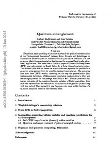
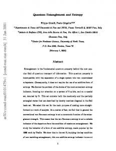
Figure 1: (a) The fiber ring connecting four buildings in Vienna and one in St. P¨olten, a city about 85 km distant from the station BREIT. (b) In general quantum networks, links represent entangled pairs of particles and any local quantum operations can be performed at the stations, which are located at the vertices of the graph. to name a few. The implementation of these concepts requires an extraordinarily careful preparation of non-classical states, which are extremely fragile against any perturbation, but the control of physical systems at the quantum scale has been impressively increased over the last few years. Advanced technologies relying on entanglement are indeed being actively developed, and quantum key distribution systems in particular have matured to real-world application. For example, quantum cryptography was used to protect voting ballots casts in Geneva (Switzerland) during parliamentary elections on October 21, 2007. Another example is given by the network consisting of five stations and seven quantum connections that has been built recently in Vienna [PPM08], see Fig. 1a. This setup operates in a point-to-point modus, which means that the stations behave classically: quantum correlations are created between neighboring stations but cannot be transmitted farther. It is nonetheless very reasonable to predict that genuine quantum networks (Fig. 1b), that is, sets of stations sharing entangled pairs of particles that can be manipulated ad libitum, will appear in the near future. Currently, remote entanglement is best created between atoms by sending single polarized photons, or beams of squeezed light, through optical fibers3 [CZKM97, Kim08]. While local operations on the quantum systems tum speed-up over classical computers is not clear at the moment [LBAW08, GFE09]. 3 A direct transmission of entangled photons over free-space links is also possible
4
Introduction
are performed more and more reliably [MHPC06, HSP10], one major challenge in quantum communication remains the generation of entanglement over a large distance. In fact, the imperfections of the quantum channels limit the maximum distance to about fifty to hundred kilometers. The two main reasons for this limited reach are the inevitable depolarization of the photons and the intrinsic loss in optical fibers [GRTZ02]. Fortunately, theoretical proposals showed that this limitation may be overcome by means of quantum repeaters [BDCZ98, DLCZ01]. In these protocols, the quantum channel is divided into smaller sections of about the size of the coherence or absorption length of the optical fibers, and entanglement is propagated by a generalized quantum teleportation called entanglement swapping [ZZHE93]. Actually, the scheme is slightly more subtle since one cannot clone nor amplify the particles (qubits) carrying the quantum information without destroying their quantum nature [WZ82]. Although the implementation of large quantum repeaters remains an ambitious task, the essential elements needed to their realization are already established [PGU+ 03, YCZ+ 08], converting the magical thought of a perfectly secure communication between distant parties into an accessible technology. In this Thesis, we study the distribution of entanglement in quantum networks in general, analyzing the generation of long-distance entanglement from an arrangement of short quantum connections in particular. We consider that neighboring stations share initially some partially entangled pairs of qubits, which emphasizes the difficulty of creating remote entanglement, and the task is then to design local quantum operations such that the entanglement present in the whole network gets concentrated between a small number of chosen stations. We will see that the geometry of the network plays a crucial role in this problem, but the real leitmotiv in this Thesis is that the best results are obtained if one “thinks quantumly” not only at the connection scale, but also from a global network perspective. In this respect, finding powerful entanglement-distribution strategies deeply depends on our knowledge of multipartite entanglement properties, that is, the characteristics of entangled states of more than two particles. The first part of the Thesis deals with a pure-state description of the quantum networks. In Chap. 1, we start by analyzing carefully the basic quantum operations that allow one to propagate or concentrate the entan[FUH+ 09], but the relevance of this method highly depends on atmospheric conditions and thus may not be appropriate in hostile environments such as cities.
Introduction
5
glement present in the links of the network. We review the entanglementswapping procedure and introduce some figures of merit to quantify its efficiency (Sec. 1.1). Then, we characterize the quantum measurements that optimally achieve this task, which leads to an interesting statement: already for systems in which only two entanglement swappings are performed, projecting onto partially-entangled states may yield better results than considering a basis of maximally-entangled pairs of qubits, see Sec. 1.2. Finally, we justify the model of the quantum connections by showing that the optimum success probability of entanglement generation between two distant stations in one-dimensional system decays exponentially with their distance (Sec. 1.3). In fact, this corresponds to the existence of an absorption (or depolarization) length in real optical fibers. In Chap. 2, we turn to two-dimensional networks, in particular to lattices in which neighboring nodes share some pure-state entanglement. The goal is to generate an entangled pair of qubits between two distant stations, and the presence of many different paths between two nodes of the lattice greatly helps in this task. In fact, if the entanglement of the connections is larger than some critical value depending on the network structure, then it can be propagated over an arbitrarily large distance. We generalize some previously known results about entanglement percolation, showing that, in some cases, quantum measurements on the nodes can increase the efficiency of the strategy (Sec. 2.2). The idea of preprocessing the entanglement percolation by a judicious choice of local quantum operations, namely a projection onto multipartite entangled states, is further developed in Sec. 2.3. This leads to a systematic improvement of the creation of entanglement over a large distance, lowering the entanglement threshold regardless of the lattice geometry. Introducing the concept of quantum complex networks (Chap. 3), we temporarily leave the problem of long-distance entanglement generation in lattices to focus on networks of richer topology. Three main properties of real-world communication networks, that are absent in regular lattices, are a small-world, clustering and scale-free behavior. The first mathematical model describing networks with the small-world property is the random graphs of Erd˝os and R´enyi (Sec. 3.1.1), and in Sec. 3.1.2 we propose a natural extension to the quantum domain. The following sections aim to show that, mainly due to the superposition principle, the quantum complex networks behave completely distinct from their classical cousins. The pure-states formalism brings a deep insight into the broad range of possibilities, but also the restrictions, of entanglement manipulation
6
Introduction
in quantum networks, However, realistic settings are best described by mixed states, since considering such quantum mixtures expresses our lack of control over all degrees of freedom of the system. The aim of Chap. 4 is twofold. First, it makes the transition between the two parts of this Thesis by showing how the results collected so far still apply for certain kinds of errors, or noise, that perturb any experiment (Sec. 4.1). Second, it briefly reviews the quantum-repeater protocols, which are proposed to create remote entanglement in noisy settings, drawing attention to their limitations (Sec. 4.2.1). In particular, the need of reliable quantum memories to store the qubits for a long time is one of the most severe problems they have to face. A new scheme for generating long-distance entanglement in quantum networks subject to general noise is presented in Chap. 5. Making full use of the geometry of two-dimensional square lattices, we combine a classical and a topological error-correcting codes into one efficient quantum protocol. All operations are performed fault-tolerantly and, equally important, simultaneously (Sec. 5.2). Therefore, the qubits have to be preserved from decoherence for a short time only, which relaxes the requirement of good quantum memories. Moreover, the overhead of local resources increases very slowly with the distance, while the tolerable error probability stays on the order of one percent for any realistic network size, making our proposal favorable for quantum communication. Finally, in Chap. 6, we prove that entanglement can be established between two infinitely distant qubits of a three-dimensional network if the noise of the connections is not too strong. To that end, we first transform the quantum state that describes the initial network into a cluster state, which is a highly-entangled multipartite state (Sec. 6.1). Then, it is shown how the information gained by measuring the qubits at each station allows one to correct most errors affecting the links of the network (Sec. 6.2). Since only a constant overhead of qubits is required per station, this strategy further lessens the physical resources that are needed for long-distance communication in quantum networks. The various results presented in Chaps. 1 and 2 have been published in [PCA+ 08], except those of Sec. 2.3 which are to be found in [PCL+ 10]. The results of Chaps. 3, 5, and 6 and the related discussions in Chap. 4 have been published in [PLAC10], [PJS+ 08], and [Per10], respectively.
Part I
Pure states
“
Making the simple complicated is commonplace. Making the complicated simple, awesomely simple, that’s creativity.
”
– Charles Mingus
Chapter 1
Entanglement manipulation in basic networks The first part of this Thesis is devoted to quantum networks in which connections are described by two-qubit entangled pure states of the form |ϕi ≡
√
ϕ0 |00i +
√
ϕ1 |11i,
(1.1)
with ϕ0 + ϕ1 = 1 and where our convention is to choose ϕ0 ≥ ϕ1 . Setting this last inequality to be strict reflects the fact that remote entanglement cannot be generated perfectly in realistic settings. On the contrary, we consider that all stations have a complete and perfect control over their particles, so that no restriction is put on the quantum operations they can perform locally. For instance, we permit the use of ancillary qubits, and no error occurs while manipulating, storing, or measuring the quantum system at a station. This may seem to be a crude approximation, but it allows one to get a deep insight into the way entanglement can be manipulated in general quantum systems. In this chapter, we study the basics of entanglement manipulation in communication networks in the very spirit of [BVK98, HS00]. The aim is to investigate and derive optimal local measurement protocols for networks consisting of few qubits only. The results obtained for these simple situations will then be used as building blocks for more elaborated schemes in larger networks. In Sec. 1.1, we start by describing the operation that propagates entanglement over a larger distance in a quantum network, namely the entanglement swapping [ZZHE93] at a node that is referred to as an entanglement swapper (or a quantum relay, see [dRMT+ 04]). This quantum operation involves a joint measurement on two qubits and is optimally performed in a basis of maximally entangled states. Depending on the figure of merit quantifying the efficiency of this procedure, however, we show that different bases (local rotation of the qubits) are to be used. In Sec. 1.2, we consider quantum systems that consist of two entan-
10
Entanglement manipulation in basic networks
glement swappers, and we find that projecting onto maximally-entangled states does not maximize, in general, the various figures of merit. In fact, the measurements at the middle stations are best performed in a basis of partially entangled states. This result, besides being rather surprising, will have some importance in the entanglement distribution protocols of the next chapter (Sec. 2.3.2). Then, we describe another useful quantum operation to manipulate the entanglement of pairs of qubits: while the entanglement swapping transfers (but inevitably decreases) the entanglement from one node to another, the distillation of several entangled states can concentrate it into one pair only. These two antagonistic effects will find a direct application in the deterministic creation of long-distance entanglement in quantum networks, see Sec. 2.1. Finally, in Sec. 1.3, we consider arbitrarily large chains of entanglement swappers. The probability to successfully generate an entangled pair of qubits between the extremities of the chain decreases exponentially with its length, which is a well-known result that is easily derived in our formalism. We then determine the exact value of the average entanglement for a specific choice of the measurement bases; it will be shown in Sec. 2.3.1 how this formula is related to the probability of creating some multipartite entangled states.
1.1
Entanglement swapping
In this section, we show how the entanglement present in single connections can be propagated over a larger distance. We introduce some figures of merit to quantify the efficiency of the procedure and describe the quantum operations yielding the optimum results. These constructions will be then extensively used to design powerful protocols for much larger systems.
1.1.1
Joint measurement at the middle station
It is a well-known result that any two-qubit entangled pure state can be transformed into the state described in Eq. (1.1) by performing a local basis rotation, which defines its Schmidt decomposition with coefficients ϕ0 and ϕ1 . We refer the reader to [NC00], for example, for the elementary definitions and notions related to quantum information theory, so that only the strictly necessary notation has to be introduced here. In Fig. 1.1a,
1.1. Entanglement swapping A a
|αi
B b0
b
Em
|βi
|φm i
a
C
11 A
c
|αi
B
C
|βi |φm i
c
|γi
D
|γi
(b)
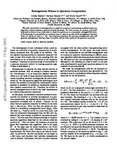
(a)
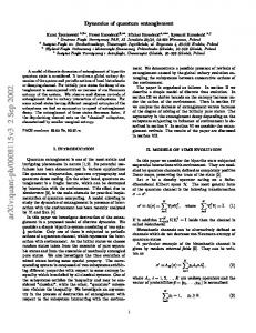
Figure 1.1: Examples of the entanglement-swapping procedure in quantum networks. (a) Entanglement can be generated between two previously unconnected stations A and C by an entanglement swapping at the middle station. We call the station B an entanglement swapper or a quantum relay. (b) Same consideration, but with two intermediate nodes. we depict one of the most primitive networks, but nevertheless important, that can be imagined. In this configuration, the central station applies a joint measurement on its two qubits, so that the extremities A and C become entangled. For instance, the station B can perform a measurement described by n positive operators Em satisfying the completeness relation Pn m=1 Em = 14 , in which case the resulting (non-normalized) state of the outcome m reads ρm ≡ tr bb0 (12 ⊗ Em ⊗ 12 ) |αβihαβ|
�
and appears with probability pm = tr(ρm ). Restricting to projective measurements P1only, that is, setting Em = |µm ihµm | for some normalized state |µm i = i,j=0 µm,ij |iji, one verifies that the smallest Schmidt coefficient of ρm is s � � 1 1 4 det(ρ0m ) 0 λm = 1− 1− , min {eigval(ρm )} = pm 2 p2m
(1.2)
with ρ0m ≡ trc (ρm ). This formula can be written in a more compact way by considering the following map from the space of two-qubit pure states to that of 2 × 2 complex matrices: |νi =
1 X
i,j=0
νij |iji
7→
νb =
1 X
i,j=0
νij |iihj| .
(1.3)
12
Entanglement manipulation in basic networks
† b and the quantities In fact, ρ0m is now given by Mm Mm with Mm = α bµ b∗m β, of interest read: √ 2 | det(Mm )| α0 α1 β0 β1 = C(µm ), (1.4a) Cm = pm pm � p 1� 2 , (1.4b) λm = 1 − 1 − Cm 2 1 X αi βj |µm,ij |2 , (1.4c) pm = i,j=0
where we have introduced the concurrence, a measure of entanglement for general states of two qubits [Woo98]. For pure states, the concurrence is defined as C(α) ≡ 2| det(b α)|. In this setting, the prototype of projective measurements is clearly the entanglement swapping, which teleports the qubit b to c by consuming the connection |βi. The measurement of the qubits b and b0 is performed in a Bell basis, which we define as follows. Starting from the computational basis { |0i, |1i}, we define two new orthogonal bases { |↑i, |↓i} and { |Φ+ i, |Φ− i, |Ψ+ i, |Ψ− i} for one and two qubits, respectively: � � � � |0i |↑i , (1.5a) =U |1i |↓i with U ∈ U(2), and |Φ± i ≡
|↑↑i ± |↓↓i √ , 2
|Ψ± i ≡
|↑↓i ± |↓↑i √ . 2
(1.5b)
The latter four vectors are known as the Bell states if no local rotation is performed, i.e., if U = 12 for both qubits. In this case, | ↑i and | ↓i are the eigenvectors of the Pauli matrix Z, and we call the basis indistinctly the Bell or the ZZ basis. Another two-qubit basis plays a key role while manipulating entangled states: the XZ basis, in which the first unitary corresponds to the Hadamard matrix, so that |↑i and |↓i are the eigenvectors of the Pauli matrix X for the first qubit. Explicitly, the ZZ and XZ bases are given by the columns of the matrices 1
MZZ
1 0 0 1 −1
1 0 =√ 2 0
1 1 1 −1 0 0 1 1 −1 1 1 1 1 . (1.6) and MXZ = 1 −1 1 1 −1 2 1 −1 1 1 1 0 0
1.1. Entanglement swapping
1.1.2
13
Figures of merit
We describe now three figures of merit that are used to evaluate the usefulness of an entanglement distribution protocol: the singlet conversion probability (SCP), the worst-case entanglement (WCE), and the average concurrence. These figures of merit take value in the interval [0, 1] and are somehow related to each other, but they present some subtle differences nonetheless. Because they are intimately related to the transformation of bipartite pure states under local operations and classical communication (LOCC), we first recall the connection between the Schmidt coefficients and majorization theory, which will naturally lead to the definition of our figures of merit. LOCC transformations and majorization theory Consider two pure states |αi and |βi in a bipartite system. Can |αi be transformed into |βi by LOCC in a deterministic way? The solution to this question was found in 1999 by Nielsen [Nie99], who noticed a connection between this problem and majorization theory. Based on this relation, Vidal extended the results to obtain the optimal probability for LOCC conversion between states whenever a deterministic transformation is impossible [Vid99]. We briefly review these results here since this formalism is widely employed in many of the protocols described in the next sections. The interesting reader is referred to [NV01] for more details. Let us introduce the concept of majorization by considering two ddimensional real vectors, v = (v0 , . . . , vd−1 ) and w = (w0 , . . . , wd−1 ), whose components are positive, sum up to one, and are sorted in decreasing order. Then v is said to be majorized by w, which is denoted by v ≺ w, if the inequalities l X i=0
vi ≤
l X
wi
(1.7)
i=0
hold for all l ∈ {0, . . . , d − 1}. The beautiful connection to entanglement manipulation between bipartite pure states is that |αi can be transformed into |βi with unit probability whenever α ≺ β, where α is the vector of Schmidt coefficients of |αi (and similarly for β). Moving now to non-deterministic transformations, the optimal probability for LOCC
14
Entanglement manipulation in basic networks
conversion is p(α → β) = min l
SCP, WCE and concurrence
(P
l αi Pi=0 l i=0 βi
)
.
(1.8)
A direct application of Eq. (1.8) is that a two-qubit state |αi, as defined in Eq. (1.1), can be converted into a singlet, or more generally into a Bell pair, with optimal probability � S(α) ≡ prob |αi 7→ |Ψ− i = 2α1 . (1.9) Explicitly, this result (also known as the “Procrustean method” of entanglement concentration [BBPS96]) is obtained by performing on one of the qubits a generalized measurement defined by the operators ! ! q q α1 α1 0 0 1 − α0 α0 and M2 = . (1.10) M1 = 0 1 0 0
Returning to the one-swapper configuration in which the central station applies some measurement operators Em , we define the corresponding average SCP as S
(2)
(α, β) ≡
n X
pm S(φm ) = 2
m=1
n X
pm φm,1 ,
(1.11)
m=1
where pm is the probability that |φm i is generated. This equation can be generalized to a system of N −1 entanglement swappers, in which case the figure of merit is denoted by S (N ) ; if the context is clear, however, we simply write S. One can also be interested in maximizing the entanglement for all outcomes, which is characterized by the WCE: W ≡ min{S(φm )}. m
(1.12)
Finally, in the same spirit, we define the average concurrence of the measurement to be n X C≡ pm C m . (1.13) m=1
In these equations, the figures of merit are defined for one measurement only, but the generalization to larger systems is straightforward: one has just to let the sum run over all possible outcomes of the various measurements.
1.1. Entanglement swapping
1.1.3
15
Optimal measurements
The power of the protocols described in the next chapters depends crucially on the efficiency of the entanglement swappings, and the choice of the measurement basis is thus of special interest. In that respect, although the Bell basis could be parameterized by four angles describing two onequbit rotations, it turns out that calculations are much easier when done in the “magic basis” [HW97] ( |Φ1 i, |Φ2 i, |Φ3 i, |Φ4 i) ≡ ( |Φ+ i, −i |Φ− i, −i |Ψ+ i, |Ψ− i). (1.14) P In this basis, in fact, concurrence of a state |νi = 4i=1 νi |Φi i sim Pthe ply reads C(ν) = 4i=1 νi2 . Since the concurrence of a Bell state is one, it follows that its components in the magic basis have all the same phase. Thus, they can be restricted to take value within the set of the real numbers. Let { |µmi} be a set of four orthogonal such states. Then the outcome probabilities given in Eq. (1.4c) read � � pm = pmin µ2m,1 + µ2m,2 + pmax µ2m,3 + µ2m,4 , (1.15a) with
pmin ≡
α0 β1 + α1 β0 2
and pmax ≡
α0 β0 + α1 β1 . 2
(1.15b)
It has to be emphasized that, given |αi and |βi and for C(µm ) = 1, these probabilities fully characterize a Bell measurement since, from Eq. (1.4), the Schmidt coefficients of the resulting states depend on pm only: s ! α0 α1 β0 β1 1 1− 1− . (1.16) λm = 2 p2m Remark that any measurement in the Bell basis yields four values pm that lie in the interval [pmin , pmax ], and let us now state and prove a reverse proposition that turns out to be very useful while maximizing the SCP: Proposition 1.1 (Bell measurements and outcome probabilities) Let {xm } be a set of four real numbers that add up to one and that lie in the interval [pmin , pmax ]. Then there exists a Bell measurement whose outcome probabilities pm are equal to xm .
16
Entanglement manipulation in basic networks
Proof First, remark that the conditions on {xm } are clearly necessary since it describes a probability distribution, and because pm = pmin κm + pmax (1 − κm ) for some κm ∈ [0, 1], see Eq. (1.15a). The degenerate situation pmin = pmax = 1/4 is trivial since it only arises if both |αi and |βi are maximally entangled. In this case, all Bell measurements yield the same outcome probabilities pm = 1/4. We thus consider pmin < pmax , and without loss of generality we sort the xm by increasing value: xi ≤ xi+1 . Let us now denote by {µm } the four vectors describing the Bell measurement in the magic basis. Since they are orthogonal, one of them is completely determined (up to a sign) by the three others; let µ4 be this vector. We parametrize the first three vectors as � √ √ √ √ µm = κm cos(θm ), κm sin(θm ), 1 − κm cos(ωm ), 1 − κm sin(ωm ) , with κm = (pmax − xm )/(pmax − pmin ), so that they are normalized and satisfy pm = xm . The remaining task is to prove that there always exist some angles θm and ωm leading to an orthogonal basis. This is straightforward if κm ∈ {0, 1} for some m, but let us write the orthogonality conditions as cos(θ1 − θ2 ) = −η1 η2 cos(ω1 − ω2 ), cos(θ1 − θ3 ) = −η1 η3 cos(ω1 − ω3 ), (1.17) cos(θ2 − θ3 ) = −η2 η3 cos(ω2 − ω3 ), p with ηm = (1 − κm )/κm . In this system, only four angles are relevant: θa = θ1 − θ2 , θb = θ1 − θ3 , ωa = ω1 − ω2 and ωb = ω1 − ω3 , which can be freely chosen in the interval [0, π]. There are, P however, some constraints on these variables. In fact, κi ≥ κi+1 and i κi = 2, so that η1 η2 ≤ 1 ∗ ∗ ∗ and η1 η3 ≤ 1. Therefore we have θa,b ∈ [θa,b , π − θa,b ], with θa,b ∈ [0, π2 ] ∗ ∗ such that cos(θa ) = η1 η2 and cos(θb ) = η1 η3 . It follows that cos(θ2 − θ3 ) is limited to the range [− cos(θa∗ + θb∗ ), 1], and one can check that there always exists at least one solution to the orthogonality conditions except if cos(θa∗ + θb∗ ) < −η2 η3 , which however never happens. In fact, this last inequality can be written in terms of κ1 , κ2 and κ3 only, which leads, after some tedious algebra, to κ1 + κ2 + κ3 > 2. But the sum of the κ’s equals two, and thus there always exists an orthonormal basis of Bell vectors leading to the probability distribution {xm }. � We have now all the tools to find the quantum operations that maximize the figures of merit of an entanglement swapping. Let us state the results in the following three propositions:
1.1. Entanglement swapping
17
Proposition 1.2 (Measurement optimizing the SCP) The measurement that maximizes the SCP after one entanglement swapping is the Bell measurement in the ZZ basis, and Smax = 2 min{α1 , β1 }.
(1.18)
Proof Two kinds of outcomes appear when performing a Bell measurement in the ZZ basis: two of the outcome probabilities are equal to pmax , while the other two are equal to pmin . Inserting these values into Eq. (1.4), one finds the corresponding smallest Schmidt coefficients: λ(pmin) =
min{α0 β1 , α1 β0 } , 2 pmin
λ(pmax ) =
α1 β1 , 2 pmax
(1.19)
whence SZZ = 2 min{α1 , β1 }. Consider now that we are allowed to jointly perform an arbitrary operation not only on b and b0 , but also on a. We are in the presence of a bipartite system, such that the results of majorization theory apply: the SCP of this system is at most 2β1 . A similar construction for the qubits b, b0 and c tells us that the SCP is at most 2α1 , so that the final SCP cannot exceed twice the minimum of α1 and β1 . � Remark that the SCP does not decrease after one entanglement swapping if we set α = β. This is the “conserved entanglement” described in [BVK99]. Proposition 1.3 (Measurement optimizing the WCE) The measurement that maximizes the WCE for a one-swapper configuration is the Bell measurement in the XZ basis: p Wmax = 1 − 1 − 16 α0α1 β0 β1 . (1.20)
Proof Supposing that the best measurement is done in the Bell basis, the result directy follows from Prop. 1.1 and Eqs. (1.6) and (1.16). In fact, one has to find a measurement that leads to four identical outcome probabilities pm = 1/4, which is achieved in the XZ basis. Now, let us prove the proposition by contradiction. Suppose that there exists a measurement described by the operators {Em = |um ihum | }nm=1 , with n ≥ 4, such that WE > WXZ . Then each λm has to be strictly greater than the smallest Schmidt coefficient of the outcomes in the XZ basis. Thus, from Eq. (1.2), det(e ρm ) > p2m 4 α0 α1 β0 β1 ∀ m. (1.21)
18
Entanglement manipulation in basic networks
Since det(e ρm ) = α0 α1 β0 β1 | det(b um )|2 , summing over m the square root of this last equation yields n X
m=1
| det(b um )| > 2.
(1.22)
We know that the concurrence of a (normalized) state is smaller than or equal to one, hence 2 | det(b um )| ≤ kum k2 . Taking the Pntrace of 2the completeness relation for P the operators Em further implies m=1 kum k = um )| ≤ 2, which is in contradiction with 4. Therefore, we have nm=1 | det(b Eq. (1.22) and thus concludes the proof. � Proposition 1.4 (Measurement optimizing the concurrence) Any Bell measurement maximizes the average concurrence of one entanglement swapping: p Cmax = 2 α0 α1 β0 β1 . (1.23) Proof It is clear from Eqs. (1.4a) and (1.13) that the maximum average concurrence is obtained for C(µm ) = 1 for all outcomes, which describes, by definition, a Bell measurement in any basis. �
1.2
Bases of maximally-entangled states are not always optimum
Entanglement is known to lie at the root of quantum communication and is often argued to be at the origin of any speed-up for quantum computation. Therefore, it seems that maximally-entangled states should be, in some sense, always the best ones to perform any basic quantum task. We have proven that this is indeed the case for one entanglement swapping, where bases of Bell pairs are used to optimize the various figures of merit. In this section, however, we show that this statement is not true in general. To that end, we investigate some systems that consist of two entanglement swappings only. An analogous result has been reported recently by Modlawska and Grudka [MG08], who have demonstrated that non-maximally entangled states can be better for the realization of multiple linear optical teleportation in the scheme of Knill, Laflamme and
1.2. Maximally-entangled states are not always optimum
19
Milburn [KLM01]. Similarly, in the context of universal quantum computation, the authors of [GFE09] conclude that entanglement must “come in the right dose”.
1.2.1
Two consecutive entanglement swappings
We consider here a system of three collinear states on which we perform two consecutive measurements, as depicted in Fig. 1.1b. In what follows, we describe the measurements that maximize the figures of merit introduced in the previous section. The maximization of the WCE and the concurrence is somehow trivial for a two-swapper configuration. First, any Bell measurement maximizes the average concurrence of the results of the two measurements. This will be generalized and proven in Sec. 1.3.1 for an arbitrary number of entanglement swappings. Second, in order to maximize the WCE, we simply perform a XZ measurement at the two central nodes. In fact, if one performs any other measurement on the first quantum relay, then at least one resulting state |φm i is less entangled than the corresponding XZ results. This further reflects in the WCE of the second measurement, which has to be a Bell measurement in the XZ basis from Prop 1.3. Let us now turn to the more interesting problem of maximizing S (3) , the average SCP of a chain of three entangled pairs of qubits and two quantum relays. The first measurement yields some states |φm i with outcome probabilities pm , while from Prop. 1.2 we already know that the second measurement has to be done in the ZZ basis. Hence, we have to find for the first quantum relay the measurement operators Em that maximize S (3) (α, β, γ) ≡ 2
X m
pm min{ϕm,1 , γ1 }.
(1.24)
We first maximize this quantity over the set of Bell measurements1 and then present some numerical results showing that non-Bell measurements sometimes yield higher values of the SCP.
20
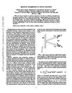
Entanglement manipulation in basic networks S (3) (α, β, γ)
h(p) 2γ1 p∗
0.4 f (p)
non-Bell
g(p)
Bell
pmin
p∗
pmax
1 2
p
S∗
(a) Graph of h, defined by S (3) = P m h(pm )
S?
1
S(α)
(b) Optimum SCP for S(β) = S(γ) = 0.4
Figure 1.2: SCP after two consecutive entanglement swappings. (a) Function h(p) = min{f (p), g(p)}, and definition of p∗ . (b) Optimal SCP as a function of the entanglement of |αi. Numerical results show that there exists a better strategy than the Bell measurements (thin line) for S(α) ∈ ]S ∗ , S ? [. The values S ∗ and S ? are such that p∗ (α∗ ) = pmin (α∗ ) and p∗ (α? ) = (1 − pmax (α? ))/3. Bell measurements We fix the states α, β, and γ and consider the SCP as a function of the outcome probabilities only: X X S (3) ({pm }) = min{f (pm ), g(pm )} ≡ h(pm ), (1.25) m
m
p
where f (p) ≡ 2γ1p and g(p) ≡ p − p2 − α0 α1 β0 β1 . One can easily verify that g(p) is strictly decreasing and convex for any states α and β: d g(p) < 0 and dp
d2 g(p) > 0 ∀ p ∈ [pmin , pmax ]. dp2
A typical example of h(p) is plotted in Fig. 1.2a, and the value p∗ at which the two functions f and g cross each other is given by: s α0 α1 β0 β1 1 . (1.26) p∗ = 2 γ0 γ1 It is sufficient to maximize the function S (3) over the set of all possible probability distributions, since Prop. 1.1 ensures the existence of a Bell 1
As we will see, this is the best strategy for a wide range of entanglement in the connections α, β and γ.
1.2. Maximally-entangled states are not always optimum p∗ versus pmin and pmax p∗ ≤ pmin
pmin ≤ p∗ ≤ 13 (1 − pmax ) 1 (1 3
∗
− pmax ) ≤ p ≤ p∗ ≥ 14
1 4
21
{pm } maximizing S (3)
strategy
{pmin , pmin , pmax , pmax }
ZZ
{p∗ , p∗ , pmax , 1 − 2p∗ − pmax } ∗
∗
∗
∗
{p , p , p , 1 − 3p } { 41 , 14 , 14 , 14 }
non-Bell Bell XZ
Table 1.1: Maximization of S (3) over the set of Bell measurements (2nd column), or performing arbitrary measurements (3rd column).
measurement leading to any such distribution. At this point, let us give three conditions that have to be satisfied by the best probability distribution: P (i) Obviously, pm ∈ [pmin, pmax ] for all outcomes m, and m pm = 1.
(ii) If the set {pm } maximizes the SCP, then all probabilities lie either to the left or to the right of p∗ . In fact, suppose for example that p1 + 2ε < p∗ < p2 − 2ε and choose p˜1 = p1 + ε and p˜2 = p2 − ε, with 0 < ε � 1. The constraints on these new probabilities are still satisfied, but a better SCP is found.
(iii) Since g is convex, if p1 and p2 are such that p∗ + 2ε < p1 ≤ p2 < pmax − 2ε, then the choice p˜1 = p1 − ε and p˜2 = p2 + ε yields a strictly greater SCP. From these considerations, it is now very simple to maximize S (3) , and one sees that the value p∗ , with respect to pmin and pmax , plays a crucial role in the choice of the optimal measurement. In fact, we have to distinguish four cases, as described in Tab. 1.1. Note that ZZ measurements lead to the maximum SCP whenever p∗ ≤ pmin , while the XZ basis is the best strategy when p∗ ≥ 1/4. So far, we have maximized the SCP after two entanglement swappings supposing that the first measurement had to be done on the states α and β. But what happens if we start from the right extremity of the chain? It appears that the maximum SCP depends, in general, on the order of the measurements, and that performing the first measurement on the most entangled states yields better results.
22
Entanglement manipulation in basic networks
General measurements The question that has still to be answered is whether or not considering bases of non-maximally entangled states leads to a better SCP than the Bell measurements. Since the concurrence of the states used for the entanglement swapping takes now any value between 0 and 1, we cannot consider S (3) as a function of the outcome probabilities only. But for a fixed concurrence C < 1 we have: p g¯(C, p) ≡ p − p2 − α0 α1 β0 β1 C 2 < g(p) ∀ p.
Marking with a bar all variables of the general measurements, we have p¯∗ < p∗ and g¯(C, p¯∗ ) < g(p∗ ). Therefore, one checks that the Bell measurements are indeed optimal except when pmin ≤ p∗ ≤ (1 − pmax )/3. The key fact about the Bell measurements in this case is that the three outcome probabilities cannot be chosen to lie on p∗ , since the fourth one would be greater than pmax . But the range of possible outcome probabilities depends on the concurrence: for example, from Eq. (1.4c), we have that p¯m ∈ [α1 β1 , α0 β0 ] for C(um ) = 0, or more generally: p¯m ∈ [¯ pmax , p¯min ] ⊇ [pmax , pmin ].
(1.27)
Hence, a better strategy is to perform a measurement such that three outcomes probabilities are equal to p¯∗ and such that the concurrences of the states are the largest ones satisfying p¯max = 1 − 3 p¯∗ . This is confirmed by a numerical optimization of the first measurement, see Fig. 1.2b, and therefore it is sometimes advantageous to use a basis of non-maximally entangled pairs of qubits to perform the entanglement swappings.
1.2.2
A single square network
We study in this section a square whose borders are four identically entangled states, see Fig. 1.3. This is clearly one of the simplest possible two-dimensional networks, and thus it is a first step towards larger systems. The task is to entangle the two opposite nodes A and D, which is done in three steps. First, the station B performs a measurement on its two qubits, and a state |βm i is created on the diagonal. Second, the station C measures its qubits in a basis that depends on m, gets a random outcome n, and therefore connects A and D with another state |γm,n i. Third, the entanglement of these two states is concentrated into one twoqubit system, a procedure which is called distillation, yielding the state
1.2. Maximally-entangled states are not always optimum
|ϕi
B
A |ϕi
|ϕi
|βm i
D C
|ϕi
A
23
|ψm,n i
|γm,n i
D
A
D
Figure 1.3: Operations on a single square network to obtain an entangled pair on its diagonal: measurements are performed at the two middle nodes, and the resulting states are distilled. |ψm,n i. The goal is of course to optimize the average entanglement of the final state, given the initial entangled links |ϕi. To that end, let us proceed backwards, starting with the optimization of the distillation. Distillation We temporarily fix the outcomes m and n, and without loss of generality we ask the corresponding Schmidt coefficients to satisfy β0 ≥ γ0 (all formulas that follow are symmetric). A straightforward application of majorization theory gives us the conditions to distill the maximum amount of entanglement from β and γ in a deterministic way: (β0 γ0 , β0 γ1 , β1 γ0 , β1 γ1 ) ≺ (ψ0 , ψ1 , 0, 0) ,
(1.28)
and the only non-trivial inequality that arises from Eq. (1.7) is β0 γ0 ≤ ψ0 . Therefore, the greatest Schmidt coefficient of the final state reads ψ0 = max
n1 2
o , β0 γ0 .
(1.29)
Optimal measurement at the station C The arguments used for the maximization of the WCE and the concurrence of a two-swapper configuration still hold here, so that XZ measurements are optimum for these two figures of merit. Applying such a measurement, we notice that a maximally entangled pair is obtained with unit probability if β0 ≤ (2β0? )−1 , where p 1 + 1 − (4 ϕ0 ϕ1 )2 ? . (1.30) β0 ≡ 2
24
Entanglement manipulation in basic networks
Entanglement of |ϕi ϕ0 ≥ ϕ∗0 ϕ?0 ≤ ϕ0 ≤ ϕ∗0 ϕ0 ≤ ϕ?0
{pm } maximizing S �
{p∗ , p∗ , pmax , 1 − 2p∗ − pmax } {p∗ , p∗ , p∗ , 1 − 3p∗ } { 14 , 14 , 14 , 41 }
strategy non-Bell Bell XZ
Table 1.2: Bell measurements at the station B that maximize S � , depending on the amount of entanglement in the connections |ϕi. Concerning the SCP, we consider a given outcome m at the station B and write the function to maximize as n1 o� X � 4 S (ϕ, β) ≡ 2 pn 1 − max , β0 γn,0 2 n n X β0 − β1 o = 2β1 + β0 2 pn min γn,1 , 2 β0 n = S(β) + β0 S (3) (ϕ, ϕ, β 0),
(1.31)
with β00 ≡ (2β0 )−1 . Consequently, all results of Sec. 1.2.1 apply here too, and the important quantities introduced in that section read pmin = ϕ0 ϕ1 , pmax = 21 − pmin , and ϕ0 ϕ1 β0 p∗ = p 0 0 = pmin √ . β0 − β1 2 β0 β1
(1.32)
4 Since p∗ is larger than pmin for all β and ϕ, it follows that Smax is reached ∗ by Bell measurements except when p < (1 − pmax )/3, see Tab. 1.1.
Optimizing the first measurement Following the best WCE strategy, one finds that� the largest Schmidt co?2 efficient of the final state is given by ψ0 = max 1/2, β0 . Therefore, a √ perfect Bell pair can be generated between A and D if β0? ≤ 1/ 2, that is, if r q √ � 1+ 1− 2 2−1 ϕ0 ≤ ϕ?0 ≡ ≈ 0.6498. (1.33) 2
1.3. An infinite chain of quantum relays
25
If this last inequality does not hold, one has to find the measurement at B that maximizes the function X 4 S � (ϕ) ≡ pm Smax (ϕ, βm ), (1.34) m
where βm is related to ϕ via Eq. (1.4). Now, we proceed exactly as for the two-swapper configuration: on the one hand we maximize S � over the set of Bell measurements, and on the other hand we show that there exist some measurement bases yielding better results for P certain states |ϕi. In � the case of Bell measurements, we write S = m h(pm ), exactly as in Eq. (1.25), and we optimize the function over the probabilities distributions {pm }. Here we make a slight abuse of notation since we denote by the same character h two different functions, which however share many similar mathematical properties. In particular, the convexity arguments used in Sec. 1.2.1 still hold in the present case. The quantity p∗ is now given by Eq. (1.32) by setting β to β ? , and therefore depends on ϕ only. In order to distinguish the various measurement strategies according to the amount of entanglement in the network, let us introduce the critical value ϕ∗0 ≈ 0.664 such that p∗ = (1 − pmax )/3. With all these definitions, one finds the optimal measurements described in Tab. 1.2, and the similarity with Tab. 1.1 is immediate. Finally, numerical results attest that Bell measurements are suboptimal in the whole range ϕ0 > ϕ∗0 , i.e., in the regime of weak entanglement. Remark, however, that measuring in the ZZ basis for nearly separable states |ϕi approaches the optimal strategy, see Fig. 1.4.
1.3
An infinite chain of quantum relays
Let us conclude this first chapter by considering a chain of N entangled pairs of qubits attached to N −1 nodes, which is the archetype of quantum communication networks since it connects arbitrarily distant stations in the most straightforward fashion. However, this one-dimensional system suffers an extremely severe limitation on the reachable communication distance: for partially entangled states, the probability of successfully generating a Bell pair between the two extremities of the chain decreases exponentially with N. Since this is one of the fundamental problems that are addressed in this Thesis, we carefully prove this statement in what follows. Moreover, the SCP after N entanglement swappings in the ZZ
26
Entanglement manipulation in basic networks S� 1
S� 1 non-Bell
0.9 Bell
0.8 S∗ S?
1
S(ϕ)
0.5
0.6
S∗ S?
S(ϕ)
Figure 1.4: Maximum SCP of the single square network. Bell measurements (thin line delimiting the shaded area) are suboptimal for the whole range of entanglement S(ϕ) < S ∗ ≈ 0.672, while a perfect singlet is obtained by performing XZ measurements if S(ϕ) ≥ S ? ≈ 0.7. Bell measurements in the ZZ basis (thin dashed line) are optimal in the regime of vanishing entanglement. basis is explicitly calculated for all N, a result that will be used in Sec. 2.3.1 for more advanced strategies in two-dimensional networks.
1.3.1
Exponential decay of the entanglement
For simplicity, let us consider that all connections have the same amount of entanglement, such that the initial chain is given by the state |ϕi⊗N . A direct generalization [VMDC04] of Eqs. (1.4a) and (1.13) yields the following result for the average concurrence of the final state: X C (N ) = 2 | det (Mm ) |, (1.35) m
with Mm = ϕ bµ b∗m1 ϕ b. . .µ b∗mN−1 ϕ, b and where the states |µmi i are associated with the measurement result mi of the i-th node. With these definitions, the maximization of C (N ) over the measurements M ≡ { |µmi i} reads: nX o � det(b µm1 . . . µ bmN−1 ) b N max max C (N ) = 2 | det(ϕ)| M
M
m
N
= |2 det(ϕ)| b ,
(1.36)
which holds for any bases of Bell pairs, i.e., if |2 det(b µmi )| = 1 ∀mi . Therefore, for non-maximally entangled connections |ϕi, the concurrence decreases exponentially with N: (N ) Cmax = (4 ϕ0 ϕ1 )N/2 .
(1.37)
1.3. An infinite chain of quantum relays (3)
p+ (2) p+ (1)
p+
1
2
(1) p−
3
(2)
(0) p±
p+
1
0 n=0
n=1
4
(1)
p+
(3) p− (1)
p−
27
(0) p+
2
0
1
(1)
(0)
p−
p+
1
(1) p−
n=3
(a) Tree describing the outcomes m
0
(1)
p+
2
0 n=2
2
(1) p−
n=0
n=1
(b) A symmetrized tree
Figure 1.5: Resulting states |ϕ(m) i after n consecutive entanglement swappings in the ZZ basis. (a) Weighted and directed tree, in which the nodes describe the labels m. (b) This tree can be made symmetric, with its root (0) (0) at n = −1, using the fact that p− = p+ = 1/2. Since the concurrence of a two-qubit pure state is always larger than or equal to twice its smallest Schmidt coefficient,2 it follows that the other two figures of merit, namely the WCE and the SCP, also decay (at least) exponentially with N. For instance, a straightforward calculation shows that Wmax behaves asymptotically as (4ϕ0 ϕ1 )N if one performs all measurements in the XZ Bell basis. This result is easily understood from the following observation: after many swappings, the entanglement of most outcomes becomes very weak, in which case the concurrence of the longdistance entangled pairs is proportional to the square root of their smallest Schmidt coefficient, leading to W ∼ C 2 . We do not have an exact formula for the maximum SCP (in the case of two entanglement swappings we already had to use numerics), but let us derive in the next section an explicit formula for the ZZ strategy.
1.3.2
Asymptotic behavior of the SCP under ZZ measurements
Measurements in the ZZ basis have been shown to maximize the SCP after one entanglement swapping (Prop. 1.2) and to be close to optimality for two quantum relays and for the single square network in the regime of weak entanglement, see Tabs. 1.1 and 1.2. It is therefore natural to consider this startegy for an infinite chain of entangled pairs of qubits, and let us compute the average SCP of the system after N swappings. 2
√ In fact, one has C(ϕ) ≡ 2 ϕ0 ϕ1 ≥ 2ϕ1 since ϕ0 ≥ ϕ1 .
28
Entanglement manipulation in basic networks
First, even if the number of outcomes grows exponentially with the length of the chain, one can keep track of all of them in an compact way. In fact, any state resulting from n ≤ N entanglement swappings in the ZZ basis has the form (up to local unitaries) √ √ m ϕ0 |00i + ϕm 1 |11i (m) √ m , m ∈ N. (1.38) |ϕ i ≡ m ϕ0 + ϕ1 This is proven by induction on n, the case n = 0 corresponding to the initial state m = 1. Suppose that the result holds and that we get the state |ϕ(m) i after n < N swappings. It is simple to show from Eq. (1.19) that a ZZ measurement on |ϕ(m) i ⊗ |ϕi yields the state |ϕ(m+1) i with (m) m |m−1| probability p+ ≡ (ϕm+1 +ϕm+1 )/(ϕm i with probability 0 1 0 +ϕ1 ) and |ϕ (m) (m) p− ≡ 1 − p+ . Then, let us calculate the variation of the SCP due to one swapping, considering that the set {(pi , |ϕ(mi ) i), i = 1, . . . , l} describes (m) the outcomes of the first n measurements. Denoting by λ± the smallest Schmidt coefficients of |ϕ|m±1| i, the new SCP reads S
(n+1)
=
l X
i=1 (n)
=S
(mi )
pi 2 p+
(mi )
λ+
(mi )
+ p−
− (ϕ0 − ϕ1 ) p(0) n ,
(mi ) �
λ−
(1.39)
(0)
where pn stands for the probability of getting the state |ϕ(0) i = |Φ+ i after n measurements. Since this probability is non null for odd n only, it results that the SCP decreases after every second swapping only. In the case n = 1, this is the “conservation of entanglement” pointed out in (0) Prop. 1.2. The quantity pn is calculated from Fig. 1.5: it is the weighted sum over all possible paths Γ that go from the root of the oriented tree to the node m = 0 at position n. We notice that the path weights, denoted by wn , depend on n only and not on the paths themselves. This (m) (m+1) is indeed the fact since p+ p− = ϕ0 ϕ1 for all m, and because the paths Γ start and terminate at the same level m = 0. Thus, for odd n we have wn = (ϕ0 ϕ1 )(n+1)/2 , and using basic combinatorial analysis one finds � (0) pn = 2k (ϕ0 ϕ1 )k , with k = 21 (n + 1) ∈ N. Finally, the average SCP after k N entanglement swappings in the ZZ basis reads S
(N )
= 1 − (ϕ0 − ϕ1 )
� 2k (ϕ0 ϕ1 )k , k
[N/2] �
X k=0
(1.40)
1.3. An infinite chain of quantum relays
29
where [x] denotes the integer part of x. This last equation behaves as √ N/2 (4ϕ0 ϕ1 ) / N for N tending to infinity, and consequently, measurements in the ZZ basis yield much better results than the XZ strategy.
Chapter 2
Long-distance entanglement in planar graphs The previous chapter concluded with the impossibility of generating longdistance entanglement in a chain of non-maximally entangled pairs of qubits. In fact, the optimum measurements lead to an exponentially small probability of success with the number of required entanglement swappings, see Sec. 1.3. However, extending the quantum network to a system of higher (spatial) dimension grandly impacts on this probability. In this chapter, we indeed show that a Bell pair can be generated over a long distance in quantum networks with the topology of planar graphs.1 More precisely, we propose some measurement strategies which yield a strictly positive probability of entangling two arbitrarily distant qubits, provided that the entanglement S(ϕ) of the elementary connections |ϕi is larger than a critical value Sc . These strategies are of two kinds, deterministic or purely statistical. While the former makes use of distillation methods, the latter exploits ideas of percolation theory. Both strategies are based on the same (and simple) observation, nevertheless: there exist plenty of weakly entangled paths between two distant nodes in a two-dimensional lattice, but only one chain of singlets is necessary to generate a Bell pair between these two nodes. In Sec. 2.1, we apply the results of the previous chapter, in particular optimal entanglement swappings and distillation procedures, to twodimensional networks of large size. We start by considering some hierarchical graphs, that is, networks that iterate certain geometric structures, so that at each level of iterations the number of nodes, or the number of neighbors, changes (Sec. 2.1.1). In particular, we discuss the “diamond” graph, for which we prove that for sufficiently large initial entanglement, 1
Basics of graph theory are supposed to be known by the reader and can be found in any textbook. For instance, we refer the reader to [Die05] for a very good but easily accessible book on this topic.
32
Long-distance entanglement in planar graphs
one can establish perfect entanglement on large scales (i.e., on some lower levels of iteration) in a finite number of steps. A similar result holds for a double binary tree, in which each iteration step branches every bond into two. For such graphs, if the initial entanglement is large enough, perfect entanglement can be established at each level of iteration. Then, in Sec. 2.1.2, we turn to genuine two-dimensional lattices. Using distillation techniques, we show that, for the square lattice, one can convert the connections of a sufficiently broad strip into a backbone of perfect singlets. Percolation strategies for infinite lattices are considered in Sec. 2.2. For instance, we reconsider the hexagonal lattice with double bonds described in [ACL07] and then discuss the case of a triangular lattice with distinct bonds. In the first of these examples, quantum measurements lead to a local reduction of the SCP but change the geometry of the lattice, which increases its connectivity and thus the classical entanglement percolation threshold corresponding to a straight conversion into singlets of all the links of the lattice. We call this effect quantum entanglement percolation. In the second example, we use the measurements optimizing the SCP to transform the original lattice into a double-size triangular lattice with a higher probability of getting a singlet on the bonds. We also describe a different type of strategies, where a square lattice is transformed into two disjoint square lattices of double size but with the same average SCP. In this case, we prove that the probability of connecting a pair of neighboring nodes to another such pair is strictly larger than in the original protocol. While the advantage of quantum entanglement percolation over the classical protocols has been found for some specific lattices only (Sec. 2.2), we propose in Sec. 2.3 a strategy that beats the classical entanglement percolation for all the lattices that we considered. This strategy is based on the creation of multipartite entangled states, see Sec. 2.3.1. It improves not only the entanglement threshold, but also the success probability of the protocol for any amount of entanglement in the connections (Sec. 2.3.3). Finally, in Sec. 2.4, we briefly discuss the optimality of the various protocols proposed for generating a long-distance entangled pair of qubits. In particular, while any percolation threshold defines a sufficient condition, it is still an open and very interesting question to determine whether or not there exists a necessary amount of entanglement to achieve this task.
2.1. Deterministic methods
2.1
33
Deterministic methods
In this section, we consider graphs in which entanglement can be generated between arbitrarily distant nodes by making us of entanglement swappings and distillations. In fact, for some graphs and if the entanglement of the connections is large enough, it is possible to compensate the loss of entanglement due to the swappings with an entanglement concentration procedure. Clearly, the distillations require that several pairs of entangled qubits are created between two nodes, which is one of the basic reasons why graphs spanning the plane are so interesting in comparison to onedimensional systems.
2.1.1
Hierarchical graphs
Let us first study the generation of entanglement over large scales in graphs that have a hierarchical geometry. These are graphs that iterate certain geometric structures, so that at each level of iteration the number of nodes (or neighbors) changes. Unfortunately, optimal strategies are not known for such graphs; we restrict our considerations to showing that one can generate perfect entanglement in a finite number of steps at some iteration level. This entanglement is further swapped to the lowest levels of iterations, i.e., to the largest scales, which can be considered as the largest geometrical distances. “Diamond” graph In this section, we consider the so-called “diamond” graph, which is obtained by iterating the following operation, see also Fig. 2.1a: a single bond (one entangled state of two qubits) is replaced by four bonds forming a diamond shape. After k iterations, the nodes A, B, C, D have 2k links, the nodes on the next level 2k−1 , etc. We now prove that for sufficiently large initial entanglement, one can establish Bell pairs on large scales in a finite number of steps. We assume that the graph is formed by many iterations and that all bonds correspond to the entangled state |ϕi. Our aim is to perform some measurements in a recursive way, showing that, for sufficiently high S(ϕ), it is possible to generate perfect entanglement on the lowest level of the iteration hierarchy, that is, between the “parent” nodes A and
34
Long-distance entanglement in planar graphs
B
B C
A
B D
A
S0 1
C
D
0.5
A Sc
(a) Construction of the diamond graph
S?
1
S
(b) Plot of Eq. (2.2)
Figure 2.1: (a) The first two iterations of the diamond graph. (b) Recursion relating S on the higher level of iteration to S 0 at one lower level of iteration. B. In order to keep the form of the network unchanged by the recursive measurements, we apply the WCE strategy to the nodes analogue to C and D, starting from the highest iteration level. The two entanglement swappings in the XZ basis yield, with unit probability, two identical pairs of entangled states which can then be distilled into a state |ψi with larger entanglement. Remark that we are exactly in the situation of the single square network discussed in Sec. 1.2.2. From Eqs. (1.20) and (1.29), one finds � �2 � p 1 1� ψ0 = max , 1 + 1 − (4ϕ0 ϕ1 )2 , (2.1) 2 4
and denoting the SCP of |ϕi and |ψi by S and S 0 , respectively, we write the recursion relation as S 2 (2 − S)2 p − 1 − S 2 (2 − S)2 , S0 = 1 + (2.2) 2
which has to be smaller than or equal to one, of course. This recursion has one unstable fixed point Sc ≈ 0.349 and two stable fixed points S = 0 and S = 1, see Fig. 2.1b. The latter is achieved in a finite number of steps, provided that the initial entanglement satisfies S > Sc . Note that Sc is strictly smaller than S ? = 2(1 − ϕ?0 ) ≈ 0.7, see Eq. (1.33), and that for S ≥ S ? the maximum entanglement S 0 = 1 is achieved in one step only. Double binary tree Similar results hold for the graph union of two binary trees, also called 3-Cayley trees, whose leaves are joined in the center, see Fig. 2.2a. Let
2.1. Deterministic methods
35 S0 S0
S S
Sˆ
S0 S0
S˜ (a)
S0
S0 (b)
Figure 2.2: (a) Two binary trees facing each other. (b) Sequence of XZ measurements and distillation leading to a recursion relation for the SCP of the bonds. us denote the initial SCP of all bonds |ϕi by S0 and perform a WCE measurement at all nodes in the middle of the tree. This prepares two twoqubit states between the neighboring nodes, which can be distilled into the pair of qubits |ψi given in Eq. (2.1). We now describe the recursion strategy, see also Fig. 2.2b: first, an entanglement swapping in the XZ basis is performed at one of the middlepnodes, which yields a state with SCP equal to Sˆ = SXZ (S0 , S) ≡ 1 − 1 − S0 (2 − S0 )S(2 − S). Then, the WCE swapping is applied to the remaining pair of bonds, leading to ˆ S0 ). Finally, the optimum entanglement distillation is applied S˜ = SXZ (S, to the pair of S˜ bonds obtained from the two different (but neighboring) branches of the tree. The recursion relation reads: n �o ˜ 2 . (2.3) S 0 = S 0 (S, S0 ) = min 1, 2 1 − (1 − S/2)
This recursion depends explicitely on S0 , and three distinct cases have to be distinguished, as depicted in Fig. 2.3:
(i) S0 < Sc : if the derivative of the recursion function is smaller than unity at the origin, then there exists only the trivial (and stable) fixed point S = 0. Explicitly, Sc is found by solving the equation �2 d 0 S (S, S ) = 2 S (2 − S ) = 1 ⇒ Sc ≈ 0.459. c c c dS S=0 Therefore, for small values of S0 , entanglement cannot be generated over a large geometrical distance.
(ii) Sc < S0 < S ? : in that case, one stable and non-trivial fixed point appears. Remark that this fixed point depends on S0 and can reach
36
Long-distance entanglement in planar graphs
S0 1
S0 1
0.5
S0 1
0.5
Sc S ? (i) S0 < Sc
0.5
1S
Sc S ?
1S
(ii) Sc < S0 < S ?
Sc S ?
1S
(iii) S0 > S ?
Figure 2.3: Recursion relation for the SCP of the double binary tree, determined by Eq. (2.3). Depending on S0 , three cases have to be distinguished. The fixed point of the recursion is highlighted by a bullet. the whole interval ]0, 1[. The value S ? is found by solving S 0 (1, S ?) = 1 and is exactly the same as for the diamond graph: S ? ≈ 0.7. (iii) S0 > S ? : if the entanglement of the bonds is large enough, then a Bell pair between distant nodes is generated in a finite number of iteration steps. Note that these considerations can be qualitatively understood from the discussion of the diamond graph, since the two constructions are quite similar and because the WCE does not increase the SCP.
2.1.2
Regular lattices
In the previous section, we have shown that entanglement can be generated over a large distance in graphs with a hierarchical structure, if the entanglement of the bonds if larger than a critical value Sc . The self-similarity of these graphs allows one to design natural sequences of entanglement swappings and distillations but suffers a physical limitation: either the length of the bonds or the number of qubits per node grows exponentially with the iteration depth. From now on, we therefore consider regular twodimensional lattices, that is, periodic configurations of nodes throughout the plane that have a finite number Z of neighbors. In what follows, we describe a deterministic strategy for lattices which have a coordination number Z strictly larger than three. In particular, we show how two infinitely distant nodes can be entangled with unit probability in the square
2.1. Deterministic methods
37 S S0
S0
Sˆ
S0
S0
S˜
S0
S0 (b)
(a)
Figure 2.4: (a) “Centipede” with its “legs” and “spine”. Remark that some bonds are not used. (b) Recursive measurement scheme; this method can be applied in higher dimensions too. lattice (Z = 4), provided a sufficiently high entanglement in the connections. The generalization to other lattices of high connectivity, such as the triangular lattice (Z = 6), is straightforward. A “centipede” in the square lattice As another example of the recursive measurement method developed in the previous section, we consider a wide stripe of a square lattice and the “centipede” figure within, see Fig. 2.4a. Let us denote the initial entanglement by S0 and the entanglement at the end bond of a “leg” by S. We sequentially shorten the legs of the centipede, gradually concentrating the entanglement of the links such that we eventually get a perfect singlet at its “spine”. Concretely, we perform on the extremity of each leg the XZ measurements depicted in Fig. 2.2b, with the difference that one of the paths has only one bond S0 and not three. The last step of the iterative procedure is then to distill two states of entanglement S0 and ˆ S0 ), with Sˆ = SXZ (S0 , S), yielding the recursion relation S˜ = SXZ (S, n S S˜ o S 0 (S, S0 ) = min 1, S + S˜ − . 2
(2.4)
This situation is very similar to the case of the double binary tree, but there is a small difference, nevertheless. In fact, the current recurrence relation depends explicitly on S0 and has always a non-trivial stable fixed point. This fixed point, however, is strictly smaller than unity when S0 is small. In this case, although we do concentrate more entanglement along the spine of the centipede, we still have to face the problem that the spine
38
Long-distance entanglement in planar graphs
(a)
(b)
Figure 2.5: (a) Horizontal centipedes of finite width can be connected at the borders of the lattice to form a giant centipede spanning one third of all the nodes (in the limit of infinite lattice size). (b) This proportion is raised to one-half by considering a spiral construction. In this case, all links of the lattice are used.
is a one-dimensional system and thus exhibits an exponential decrease of the SCP with the number of entanglement swappings that are required. On the other hand, if S0 is larger than the critical value Sc ≈ 0.649, then the fixed point is a maximally-entangled state. This point is reached in a finite number of iteration steps; note that Sc is simply the smallest value such that S 0 (1, Sc ) = 1. The construction of the centipede, as proposed in Fig. 2.4a, implies that only the nodes lying on the (one-dimensional) spine can get entangled. It may therefore seem a huge waste of physical resources, since the ratio between the number of final Bell pairs and the consumed ones approaches zero for a lattice size tending to infinity. However, this observation is pertinent only close to the critical point Sc . In fact, for sufficiently large entanglement in the initial bonds, the width of the centipede, which is equal to twice the length of its legs, is very small. For instance, one can check that only one iteration step is necessary to get a maximally entangled pair if S0 ≥ S ∗ ≈ 0.684, which is the solution of S 0 (S ∗ , S ∗ ) = 1. In that case, many narrow centipedes can be created and, more important, connected together, as depicted in Fig. 2.5a. It follows that the resulting “giant” centipede spans a non-vanishing proportion of all the nodes, which tends to one third in the limit of infinite lattice size. Remark that this ratio is further increased to one-half by considering a slightly different measurement pattern, see Fig. 2.5b.
2.2. Strategies based on bond percolation
2.2
39
Strategies based on bond percolation
The strategies that have been proposed so far to achieve long-distance entanglement in two-dimensional networks are based solely on two properties of the pure states. First, entanglement can be propagated (at high cost) through the lattice with the help of entanglement swappings. This is equivalent to performing a sequence of teleportations having each a non-unit probability of success: one station prepares locally an entangled pair of qubits, one of which is sent from node to node until it reaches its destination. The second ingredient is that multiple connections between two nodes can be distilled, compensating (or even surpassing) the loss of entanglement due to the swappings. Thus, the minimum requirement for generating long-distance entanglement with this strategy is that a “backbone” of Bell pairs is created in the lattice. This is possible if the initial entanglement of the bonds is larger than a critical value Sc and if the nodes that belong to the backbone have at least four neighbors each: two connections are part of the backbone, while the other two are used to distill the former. Since deterministic strategies typically create a one-dimensional chain of Bell pairs by using only a stripe of finite width from the lattice, they do not seem to exploit the full potentiality of twodimensional networks. These considerations raise at least two important questions: how can one deal with lattices of small connectivity (as the honeycomb lattice for example), and can the critical value Sc of the deterministic methods be lowered by using other strategies? An affirmative answer to these questions was given [ACL07], bringing ideas of percolation theory to the context of quantum communication networks.2 In Sec. 2.2.1, we present the basics and some well-established results of classical percolation theory and recall the entanglement percolation protocols proposed in [ACL07]. Those are of two types: first, the so-called classical entanglement percolation (CEP) protocols, in which the quantum links |ϕi of the lattices are converted into singlets with optimum probability p = S(ϕ). This defines a (classical) percolation problem where bonds 2
Note that the probabilistic nature of quantum physics makes percolation theory a particularly well-adapted toolbox for the study of quantum systems subject to measurements for instance. Ideas of percolation theory are for example useful in the context of quantum computing with non-deterministic quantum gates [KRE07]. The interested reader is referred to pp. 287–319 in [SBC09] for an overview of the application of percolation methods to the field of quantum information.
40
Long-distance entanglement in planar graphs
p = 0.25
p = 0.50
p = 0.75
Figure 2.6: Classical bond percolation: bonds are open (present) with probability p and closed otherwise, and groups of nodes connected by open bonds are called clusters. In these examples, the largest cluster is highlighted: typically, it is small and bounded for p < pc but spans a finite proportion of the lattice for p > pc (the critical value pc is equal to 50% in infinite square lattices). In the latter case, the largest cluster is written C and is called the giant cluster. are inserted with probability p in the lattice. Second, in Sec. 2.2.2, we develop the ideas of [ACL07] showing that CEP strategies can be surpassed, in some cases, by quantum entanglement percolation (QEP) protocols. In this scenario, joint measurements are previously performed at the nodes of the lattice. In particular, the fact that the average SCP does not decrease after one entanglement swapping allows one to define a bond percolation problem in a new lattice that has a favorable geometry. Such structural transformations have been further elaborated in [LWL09] and expanded to complex networks [CC09] and to bipartite mixed states [BDJ09].
2.2.1
Classical entanglement percolation
Classical percolation is perhaps one of the most fundamental examples of critical phenomenon, since it is a purely statistical one [Gri99]. At the same time, it is very universal, since it describes a whole variety of physical, biological or ecological processes; see [SA91] for a nice introduction to percolation theory. In bond percolation, we typically consider a regular lattice of nodes connected by random bonds, the probability of having a bond between two neighboring nodes being p, see Fig. 2.6. For a given infinite lattice, one would like to know whether an infinite open cluster exists, that is, whether there is a path of connected nodes of infinite length
2.2. Strategies based on bond percolation
41
through the lattice. It turns out that an unique giant cluster appears if, and only if, the connection probability p is larger than a critical threshold pc , which depends on the lattice. Few lattices have a threshold that is exactly known; among them we find the important honeycomb, square, and triangular lattices [SE64]: p7 c = 1 − 2 sin(π/18),
p2 c = 1/2,
and pMc = 2 sin(π/18).
In this chapter, we extensively use such results of percolation theory, and we refer the reader to the above-cited books or to [BR06] for mathematical definitions and rigorous proves. Suppose that we want to generate entanglement between two distant stations A and B in a quantum lattice, where each connection denotes a non-maximally entangled state |ϕi. Classical entanglement percolation runs as follows [ACL07]: every pair of neighboring nodes optimally converts its two-qubit state |ϕi into a Bell pair, which succeeds with probability S(ϕ), see Eq. (1.9). If this value is larger than the threshold pc of the lattice, i.e., if S > Sc ≡ pc , then a giant cluster C appears, and the probability that both A and B belong to C is strictly positive. In that case, one can find a path of singlets between the two nodes and perform the necessary entanglement swappings such that A and B become entangled. Note that this path is randomly generated by the measurement outcomes at the nodes, which contrasts with the deterministic methods described in the previous section. At this point, let us be a little more precise and define the quantities characterizing long-distance entanglement. A quantity of primary interest, very related to the percolation threshold, is the percolation probability θ(p) ≡ P (A ∈ C),
(2.5)
being the probability that a given node A belongs to the giant cluster. Clearly, θ(p) = 0 for p < pc , while θ(p) > 0 for p > pc . In quantum communication, we are interested in the probability P (A � B) of creating a Bell pair between two nodes A and B separated by a distance L. For p < pc , this probability decays exponentially with L/ξ(p), where the correlation length ξ(p) describes the typical radius of an open cluster. Above the critical point, the two nodes are connected only if they are both in C. In the limit of large L, the events {A ∈ C} and {B ∈ C} are independent, which, together with translational invariance, reduces the problem
42
Long-distance entanglement in planar graphs
(a)
(b)
Figure 2.7: Each bond of the honeycomb lattice consists of two copies of the state |ϕi. (a) The dashed nodes perform three optimal entanglement swappings according to the SCP. (b) A triangular lattice of identical average SCP is obtained, and classical entanglement percolation is now possible in this new lattice. to studying θ(p): P (A � B) = θ2 (p).
2.2.2
(2.6)
Quantum entanglement percolation
A natural question one may ask is whether the thresholds Sc defined by classical percolation theory are optimal. In fact, entanglement percolation represents a related but different theoretical problem, where new bounds may have to be obtained. This is of course equivalent to determine if the measurement strategy based on local SCP is optimal in the asymptotic regime. Here, we construct several examples that go beyond the classical percolation picture, proving that the classical entanglement percolation strategy is not optimal. The key ingredient for the construction of these examples is the measurement strategy obtained for the one-swapper configuration that maximizes the SCP, namely the entanglement swapping in the ZZ basis (Prop. 1.2). Honeycomb lattice with double bonds The first example, which was already discussed in [ACL07], considers a honeycomb lattice where each pair of neighboring nodes is connected by two copies of the same two-qubit state |ϕi, see Fig. 2.7a. The CEP strategy converts in the best possible way all bonds shared by two parties
2.2. Strategies based on bond percolation
43
into one singlet. Majorization theory tells us how much entanglement can be distilled from each double bond in case of weak entanglement, namely S( |ϕi⊗2) = 2(1−ϕ20 ), see Eq. (1.29). We choose this conversion probability to be equal to the percolation threshold for the honeycomb lattice, which results in an entanglement threshold Sc for the state |ϕi: ! ! r r �π� p7 1 Sc = 2 1 − 1 − c =2 1− ≈ 0.358. (2.7) + sin 2 2 18 Now, we show that there exists a QEP strategy yielding a better percolation threshold: half the nodes perform on their qubits three entanglement swappings in the ZZ basis, mapping the honeycomb lattice into a triangular lattice as depicted in Fig. 2.7b. The important ingredient of this construction is that the SCP of the new bonds is exactly the same as the SCP of the initial state |ϕi. We set its entanglement to be pMc , and a lower threshold is found: �π� Sc = pMc = 2 sin ≈ 0.347. (2.8) 18 This proves that CEP is not optimal since it cannot generate long-distance entanglement if 0.347 < S(ϕ) < 0.358, while the proposed QEP strategy achieves it with a strictly positive probability. Asymmetric triangular lattice A second example, although less symmetric, is generic and has a totally different character than the previous one. For simplicity, we show the argument in the case of a triangular lattice, but the same reasoning can be applied to other geometries. Consider the asymmetric triangular lattice depicted in Fig. 2.8a. A solid line corresponds to the two-qubit pure state |ϕi, while a dashed line represents a less entangled state |ϕi, ˜ i.e., S > S˜ (with obvious notation). We choose the first state such that its √ amount of entanglement satisfies pMc < S < pMc . If |ϕi ˜ = |ϕi, the classical entanglement percolation strategy works. However, we tune the entanglement of the second state such that its SCP is small enough to make the classical entanglement percolation impossible. Such a tuning always exists. In fact, we note that when S˜ → 0, these states can simply be removed from the lattice, and classical entanglement percolation fails since we have S 2 < pMc and because the links of the new lattice consists of two consecutive states |ϕi. It is now straightforward to construct a
44
Long-distance entanglement in planar graphs
(a)
(b)
Figure 2.8: An asymmetric triangular lattice. (a) The lattice consists of two different entangled states |ϕi and |ϕi, ˜ drawn in solid and dashed lines, respectively. The less entangled states |ϕi ˜ are discarded, and some of the nodes perform an entanglement swapping in the ZZ basis. (b) A new triangular lattice is obtained, solely governed by the SCP of |ϕi. successful QEP strategy: the states |ϕi ˜ are discarded and the optimal SCP strategy for one entanglement swapping is performed, see Fig. 2.8b. The lattice is transformed into another triangular lattice, in which all links have the same amount of entanglement S > pMc , so that CEP can now be successfully applied. Doubling the square lattice The final example has yet another character and deals with a square lattice in which all bonds are identical and described by the state |ϕi. Here, we replace every second pair of horizontal bond by a single one performing an entanglement swapping in the ZZ basis; let us recall that this operation does not decrease the average SCP of the bonds (Prop. 1.2). The same is done with every second pair of vertical bonds, and we consequently replace the original square lattice by two disjoint lattices having a lattice constant that is twice larger than the original one, see Fig. 2.9. Now, we are interested in establishing long-distance entanglement between A or A0 and B or B 0 . The nodes A and A0 (B and B 0 ) are next-nearest neighbors in the original lattice but belong to different double-size lattices. Let us first consider the QEP strategy for which calculations are simple. The pairs (A, B) and (A0 , B 0 ) belong to two disjoint lattices, and the probability that one of these pairs belongs to the percolating cluster is asymptotically equal to θ2 (p), with p = S(ϕ). The probability that at
2.2. Strategies based on bond percolation
45
A A0
(a)
(b)
Figure 2.9: (a) Measurements doubling the lattice constant of the square lattice: the dashed nodes perform an entanglement swapping along the vertical and horizontal directions. (b) Two disjoint square lattices with double lattice constant are created, and we want to establish an entangled pair of qubits between A or A0 and B or B 0 (not shown). least one of the pairs belongs to the giant cluster is thus PQEP = 1 − (1 − θ2 )2 = θ2 (2 − θ2 ).
(2.9)
This probability has to be compared with the CEP probability that at least one of the pairs (A, B), (A0 , B), (A, B 0 ) or (A0 , B 0 ) belongs to the giant cluster in the original square lattice. Asymptotically, it is given by PCEP = π 2 , where π is the probability that A or A0 (or equivalently B or B 0 ) belongs to the giant cluster: π = P (A ∨ A0 ∈ C) = P (A ∈ C) + P (A0 ∈ C) − P (A ∧ A0 ∈ C).
(2.10)
In order to estimate the last term in the above expression, we use the celebrated Fortuin–Kasteleyn–Ginibre (FKG) inequality [FKG71]. To that end, we first recall the following definition: an event described in terms of a percolation configuration is said to be increasing if it has the property that, once it holds for a certain bond configuration, it holds for all configurations obtained by adding bonds to the initial one. The FKG inequality then states that any two such events are positively correlated. The events {A ∈ C} and {A � A0 } (“A and A0 are connected by a path of maximally entangled bonds”) are clearly increasing, and since their intersection is the event {A ∧ A0 ∈ C}, it follows that P (A ∧ A0 ∈ C) ≥ P (A ∈ C) P (A � A0 ).
(2.11)
46
Long-distance entanglement in planar graphs
Denoting P (A ∧ A0 ∈ C) by τ , we verify that π ≤ θ(2 − τ ), and therefore doubling the square lattice is a better strategy than the classical percolation, i.e., PQEP ≥ PCEP , whenever (2 − τ )2 ≤ 2 − θ2 .
(2.12)
Let us show that this inequality holds when p lies just above the threshold p2 c = 0.5. √ In that case, θ tends to zero, and we thus have to show that τ ≥ 2 − 2 ≈ 0.586. We may try to estimate τ from below by considering the six shortest trajectories connecting A and A0 : the most direct ones (two paths of length two), and the two pairs of four-bond paths around the adjacent squares. This leads to τ > 2q − q 2 , with q = p2 + 2p4 − 2p5 . Unfortunately, for p = 0.5, this estimate is too small and thus not sufficient to our purpose. In fact, it gives only τ > 0.527. One can improve the estimate analytically by adding further paths connecting A and A0 . This procedure becomes, however, technically tedious, and we therefore turn to a standard numerical Monte Carlo simulation for calculating the transition probability from A to A0 . The method we use generates the shortest paths (like the ones used for calculating the above estimate) automatically, while the longer ones are introduced by the Monte Carlo sampling. For p > p2 c, the convergence is exponential: if we plot a subsequent estimate of τ as a function of the maximum cluster size allowed in the Monte Carlo sampling, it approaches the final value exponentially fast for large clusters. As expected, the convergence is algebraic at p = p2 c : the estimate of τ approaches its final value as a power of the cluster size. A power law fit and a comparison with the values just above the percolation threshold give, with a very good accuracy, τ ' 0.687. This proves that quantum mechanical measurements can improve the classical percolation strategy. In this example, the QEP protocol does not lead to a better threshold but yields a higher probability of generating a long-distance Bell pair for p approaching p2 c from above. Note that the inequality PQEP > PCEP also holds for all p ∈]p2 c , 1[, as recently shown in Sec. IIIC of [LWL09].
2.3
Multipartite entanglement percolation
In the previous section, we have shown how CEP can be enhanced by previously applying some quantum operations at the nodes. All examples given so far consist of transforming the quantum lattices by a sequence of entanglement swappings in the ZZ basis, thus conserving the average
2.3. Multipartite entanglement percolation
47
entanglement of the bonds. These examples are, however, restricted to pure geometrical transformations, and apply to some specific lattices only. In this respect, it is not clear whether or not the CEP strategy, and particularly the corresponding threshold, can be improved in the simple square or triangular lattices for instance. In this section, we introduce a powerful class of QEP strategies that exploit multipartite entanglement. In contrast to the protocols designed in Sec. 2.2.2, which solely employ entanglement swappings and conversions into singlets, we make full use of both the classical and quantum aspects of a quantum network: connectivity of the nodes and multipartite entanglement, respectively. The interplay of geometrical lattice transformations and entanglement manipulations is in fact a key ingredient in surpassing CEP. In Sec. 2.3.1, we generalize the usual entanglement swapping to the case of three or more qubits. This quantum operations naturally introduces the Greenberger-Horne-Zeilinger (GHZ) states |0i⊗n + |1i⊗n √ , (2.13) 2 which are the generalization of the Bell pair |Φ+ i to n qubits. Then, in Sec. 2.3.2, we describe how GHZ states can percolate in a quantum lattice, leading to a site rather than a bond percolation process. Finally, we show in Sec. 2.3.3 that this multipartite strategy systematically outperforms the CEP method, regardless of the initial entanglement of the bonds and of the lattice geometry. If in the previous section it was difficult to contrive an example where CEP can be surpassed, it is now hard to find an example that does not admit any improvement. Indeed, multipartite entanglement percolation leads to higher connection probabilities for all the lattices that were considered. |GHZn i ≡
2.3.1
Generalized entanglement swapping
The basic quantum operation that creates entanglement between the extremities of two entangled pairs qubits is a measurement of the middle qubits, as discussed in Sec. 1.1.1 (see also Figs. 1.1a and 2.10a). The main and simple (but powerful) idea of this section is to replace the complete measurement at B by a generalized measurement B with operators B0 = |0ih00| + |1ih11| , B1 = |0ih01| + |1ih10| ,
(2.14)
48
Long-distance entanglement in planar graphs
(a)
(b)
Figure 2.10: Generalized entanglement swapping. (a) Two partially entangled pairs of qubits are probabilistically converted into a GHZ state of three qubits. (b) Two (or more) GHZ states can be merged into a larger structure. Here, we depict the operation |GHZ3 i⊗2 → |GHZ5 i.
P which satisfy the completeness relation 1i=0 Bi† Bi = 14 . The second outcome leads to a perfect GHZ state among the three nodes (after a bit-flip X at C), but with probability ϕ20 + ϕ21 the first outcome yields the (unnormalized) state ϕ0 |000i + ϕ1 |111i. As for a pair of qubits, the latter state is transformed into |GHZ3 i with probability 2ϕ21 /(ϕ20 + ϕ21 ). Summing the two possibilities, we find that two copies of |ϕi are converted into one GHZ state of three qubits with optimal probability 2ϕ1 . The multipartite method derives its power from the fact that, while the value of this probability is the same as for the two-qubit swapping used in previous entanglement percolation protocols, we now have three entangled qubits rather than two. The above procedure can be generalized to construct GHZ states of n+ 1 qubits starting from n copies of |ϕi sharing a common node. In this case, we apply 2n−1 measurement operators Em of the form |0ihm| + |1ihm| , where m is the complement of m written in base 2. With a little thought, one sees that this generalized measurement is equivalent to a sequence of n − 1 entanglement swappings in the ZZ basis, exactly as for a chain of n partially-entangled states. It follows that the probability of creating a GHZ state of n + 1 qubits is given by Eq. (1.40) with N = n − 1, that is, P (GHZn+1 ) = S (n−1) . Remark that this construction is optimal for n = 3 only, and that higher success probabilities can be found by considering different measurement bases, as discussed in Sec. 1.2.1. Suppose now that two perfect GHZ states of size n and m have been created in the lattice, and that they share one common node, say B. One can then build a larger GHZ state on n + m − 1 nodes with unit probability by performing the generalized measurement B on the two qubits of B and by applying some
2.3. Multipartite entanglement percolation
49
bit-flips X depending on the outcome (see Fig. 2.10b): LOCC
|GHZn i ⊗ |GHZm i −−−−→ |GHZn+m−1 i. prob=1
Finally, let us remark that, given a GHZ state of any size, a perfect Bell pair is created between any two of its qubits by measuring all other qubits in the X basis. GHZ states, CEP, and classical pathfinding algorithms Before turning to multipartite entanglement percolation, let us show that the creation of GHZ states can also be useful in the last step of the CEP protocols. In fact, after the conversion into singlets of the bonds of the lattice, we have to find a path between the two distant nodes A and B that want to share a Bell pair (we consider that both belong to the giant cluster). Then, every node lying on this path has to behave as an entanglement swapper. There exist efficient classical algorithms to find the shortest path between two nodes in a graph, as the one proposed by Dijkstra in [Dij59], but the time required to solve this problem scales with the size of the lattice. It follows that, right after the singlet conversion, the nodes do not know if they further have to perform an entanglement swapping on some of their qubits. Instead of waiting for this information to come, every node but A and B can apply a GHZ measurement on the qubits that belong to a successfully converted Bell pair. These local operations create a “giant” GHZ state spanning the lattice, which is done in a time that does not scale with the lattice size. Hence, quantum correlations between A and B are already available before the (time-consuming) classical processes occur, which may be favorable in the context of quantum key distribution for instance [GRTZ02]. Remark that the outcome results of all sites that belong to the giant cluster are still required (at some later time) to deduce which of the Bell states was used for creating the quantum correlations between A and B.
2.3.2
An illustrative example
Let us consider a honeycomb lattice whose bonds are given by the partially entangled state |ϕi. In what follows, we first show how the multipartite strategy improves the entanglement threshold, which is related to a natural
50
Long-distance entanglement in planar graphs
(a)
(b)
(c)
Figure 2.11: From bond percolation in the honeycomb lattice to site percolation in the triangular lattice. (a) In the honeycomb lattice L, half the nodes apply a GHZ projection on their qubits. (b) GHZ states of four qubits (triangles) are created with probability pˆ each. (c) The entanglement threshold is related to the site percolation threshold in a new lattice Lˆ (here, the triangular lattice). site percolation process.3 Then, we carefully describe how the efficiency of CEP is compared with that of the multipartite protocol. Entanglement threshold: from bond to site percolation Each second node of the honeycomb lattice L performs a generalized entanglement swapping on its three qubits, as depicted in Fig. 2.11a, which creates a state |GHZ4 i with probability4 pˆ = P (GHZ4 ). We then define a ˆ in which the vertices represent the GHZ states, and where new lattice L, two vertices are connected by a bond if the corresponding GHZ states share a common node in L, see Figs. 2.11b and 2.11c. Adopting the usual terminology, we say that a site is open in Lˆ if the GHZ transformation succeeded and closed otherwise. Since two GHZ states sharing one common node can be merged into a larger connected structure, it is easy to see that long-distance entanglement is possible if the corresponding site ˆ In the present case, Lˆ is the percolation leads to a giant cluster in L. triangular lattice, whose site percolation threshold is equal to one-half, 3
Note that bond percolation can always be “artificially” mapped to site percolation. ˆ For clarity, all percolation parameters marked with a circumflex, such as pˆ or θ, refer to multipartite entanglement protocols. 4
2.3. Multipartite entanglement percolation
51
see [BR06] for instance. Therefore, a giant GHZ state appears if ˆ pˆ(ϕ) > psite c (L).
(2.15)
In the present example, performing the generalized entanglement swapping in the computational basis is not sufficient to beat the CEP threshold. In fact, since it corresponds to two consecutive swappings in the ZZ basis, one finds from Eq. (1.40) that the entanglement threshold Sˆc for this multipartite strategy, which is found by solving pˆ(ϕ∗ ) = 6(ϕ∗1 )2 − 4(ϕ∗1 )3 =
1 = psite c (4), 2
(2.16)
is exactly equal to the CEP threshold Sc in the original lattice: Sˆc = 2ϕ∗1 = 1 − 2 sin(π/18) = pbond (7) = Sc . It is in fact a pure coincidence that both c Sˆc and pbond (7) are solution of the algebraic equation 1 − 3x2 + x3 = 0, c which, in the latter case, arises from the so-called star-delta transformation [SE63, SE64]. However, we know from Sec. 1.2.1 that the bases for the generalized entanglement swapping can be optimized, increasing the probability pˆ of creating the GHZ states. For instance, optimizing these measurements over the Bell bases indeed yields Sˆc ≈ 0.6182, which is smaller than Sc ≈ 0.6527. Finally, the entanglement threshold can be made even smaller by considering non-Bell measurements, see Tab. 1.1: a numerical optimization leads to Sˆc ≈ 0.6090, which clearly beats the CEP strategy. Long-distance entanglement above the percolation threshold The minimum amount of entanglement necessary to create a long-distance entangled pair is obviously a very interesting question, but it is also important to quantify the efficiency of the protocol for a given resource |ϕi; in what follows, we shall assume that its entanglement lies above the percolation threshold. As discussed in the previous sections, the quantity of interest is P (A � B), which, for CEP, reduces to the study of the percolation probability θ(p) through the equation P (A � B) = θ(p)2 . Since multipartite measurements change the topology of the underlying ˆ p), such lattice, one has to define carefully the corresponding quantity θ(ˆ 2 ˆ ˆ that P (A � B) = θ (ˆ p) holds for very distant nodes A and B. In fact, one cannot consider the usual percolation probability in the transformed lattice, because the new vertices are not directly related to the nodes of
52
Long-distance entanglement in planar graphs
the original lattice. For this reason, it is clearer to consider the creation of the GHZ states in the original lattice, as depicted in Fig. 2.11b. We ˆ p) to be the probability that a node is connected to the giant then define θ(ˆ GHZ state, or equivalently, that at least one of the GHZ connected to this node is successfully created and belongs to the giant cluster. In terms of ˆ we have for the probability measure on the site percolation process on L, a node A: ˆ p) ≡ Pˆ (∪i {Aˆi ∈ C}), ˆ θ(ˆ (2.17) where the union is over all the sites Aˆi possessing a qubit that is also ˆ p) now depends on the choice of A, since the nodes in A. Note that θ(ˆ which did not perform any multipartite measurement are surrounded by three GHZ states, while the others are connected to one GHZ state only. For the multipartite strategy, we therefore restrict the two nodes to be chosen only from those at which no generalized entanglement swapping ˆ p) depend on the sites is to be made. More generally, both θ(p) and θ(ˆ of the lattice, so that we consider only the nodes for which these values are maximum. We denote by f and fˆ the fraction of such nodes in L ˆ respectively, which allows a fair comparison between CEP and the and L, multipartite protocols. In fact, the latter strategy always consumes some nodes for the creation of the GHZ states, and consequently we have f < fˆ, in general. Finally, the percolation probabilities are calculated by Monte Carlo simulations, showing that the multipartite strategy not only leads to a better threshold than CEP but is also favorable in the whole range S ∈ [Sc , 1), see Sec. 2.3.3 (a different measurement pattern is used there, however). Percolation probability close to unity Let us consider the regime in which the connections are highly entangled, i.e., p = 2ϕ1 = 1−ε with ε � 1. In that case, clearly, we also have pˆ = 1−ˆ ε with εˆ � 1, but one can verify that εˆ > ε for any GHZ measurement involving more than two links. An analytical study of the percolation probabilities becomes possible in this regime of entanglement, and we use the perimeter method to compute high-density series expansions of θ(p) ˆ p). The reader is referred for instance to App. C in [LWL09] for a and θ(ˆ description of this method, but for completeness let us explain it in the present situation. From Fig. 2.11b, it is clear that at the lowest order ˆ p) = 1 − εˆ3 + O(ˆ in εˆ one finds θ(ˆ ε4 ). In fact, since a node that did not perform any measurement is connected to three GHZ states (those are
2.3. Multipartite entanglement percolation
53
created with probability pˆ each), its probability not to be connected to the giant cluster is, at this order, given by (1 − pˆ)3 = εˆ3 . One can further compute the next non-trivial order of the percolation probability by the following reasoning. Suppose that exactly one out of the three GHZ states is successfully generated. Then the node is disconnected from the giant cluster if the multipartite conversion failed for all neighboring nodes, which occurs with probability (1 − εˆ) εˆ6 ≈ εˆ6 . Because this situation happens independently three times, we finally get ˆ p) = 1 − εˆ3 − 3ˆ θ(ˆ ε6 + O(ˆ ε7 ).
2.3.3
(2.18)
The superiority of multipartite strategies
Now that the basic ingredients have been presented, we show that multipartite strategies outperform all previously known classical or quantum strategies, regardless of the initial entanglement of the bonds and for every lattice that we considered. From the above discussion on the percolation probability close to unity, a necessary condition for this statement to hold is that the measurement pattern does not comprise generalized entanglement swappings on more than two links. We hence focus on the measurements described in Eq. (2.14), such that pˆ = p = 2ϕ1 . This section is structured as follows. First, we list the various lattices that are considered, and we carefully describe the measurement patterns that are applied on them. Second, we examine the thresholds and show ˆ that pˆc < pc for each lattice. Then, we compute the expansions θ(p) and θ(p) in the high-density (i.e., maximally-entangled) limit to prove that ˆ θ(p) > θ(p) as p tends to unity. Finally, using Monte Carlo techniques, we show that Pˆ (A � B) > P (A � B) for all p > pˆc . Lattice transformations and percolation thresholds We start by considering the (4, 82) Archimedean lattice,5 see [GS86] for this notation. In the first panel of Fig. 2.12, we propose a measurement pattern indicating on which qubits the generalized entanglement swapping is applied: the new lattice is denoted by 2/3 (32 , 62 ) + 1/3 (3, 6, 3, 6), and its 5
An Archimedean lattice is a tiling of the plane by regular polygons, in which each vertex is surrounded by the same sequence of polygons (here, one square and two octagons).
54
Long-distance entanglement in planar graphs
(4, 82 )
Hexagonal
Square
(32 , 4, 3, 4)
Kagom´e
Dice
Bowtie
Triangular
Figure 2.12: Lattice transformations under generalized entanglement swappings. Some nodes (filled circles) perform one or more GHZ measurements on their qubits, which are not drawn for clarity. Nodes where no quantum operation is performed (empty circles) are used for computˆ Finally, in the (32 , 4, 3, 4) lattice, some ing the percolation probability θ. of the links (dashed lines) are simply converted into Bell pairs as in CEP.
2.3. Multipartite entanglement percolation
55
#
Lattice
pc
pˆc
∆ [%]
1 2 3 4 5 6 7 8
(4, 82 ) Hexagonal Kagom´e Square Dice (32 , 4, 3, 4) Bowtie Triangular
0.6768 0.6527 0.5244 0.5000 0.4755 0.4141 0.4045 0.3472
0.6499 0.609(0) 0.427(1) 0.392(8) 0.375(5) 0.344(7) 0.294(9) 0.273(5)
4.0 6.7 18.6 21.4 21.0 16.8 27.1 21.2
Table 2.1: Improvement of the entanglement percolation thresholds using a multipartite strategy, and relative gain ∆ ≡ 1 − pˆc /pc . We performed Monte Carlo simulations to calculate pˆc for the lattices 2–8. All other values are to be found, with higher precision, in [Gri99, Par04, NMW08].
critical point is pˆc ≈ 0.6499 [NMW08]. Since the original threshold is pc ≈ 0.6768 [SZ99], the proposed strategy yields an improvement over CEP. It is interesting to note that the transformed lattice, arising from simple quantum operations, is among the rather exotic examples considered in other studies. For example, this two-uniform lattice is considered in [NMW08], where a quantitative relation between percolation thresholds and the Euler characteristic is demonstrated. We studied many other lattices and found that multipartite entanglement percolation leads to better thresholds than CEP in every case, which suggests that it may be a universal result. All the lattices that were considered are depicted, together with the corresponding measurement patterns, in Fig. 2.12. Many such patterns lead to an improvement over the CEP strategy, but for simplicity we considered only periodic ones. For the square lattice, for instance, one can pair the links in such a way that two overlapping square lattices of double size are created. The key advantage of the multipartite strategy, with respect to the construction described in Fig. 2.9, is that we do not get disjoint lattices anymore, but rather connected ones since the middle qubits can be used to propagate the entanglement through the network. We did not find published values of the site percolation thresholds in the resulting lattices, mainly because they are non-planar or non-regular
56
Long-distance entanglement in planar graphs
#
θ
θˆ
f
1 2 3 4 5 6 7 8
1 − ε3 − 4ε4 − 11ε5 1 − ε3 − 3ε4 1 − ε4 − 6ε6 1 − ε4 − 4ε6 1 − ε6 − 6ε7 1 − ε5 − 5ε8 1 − ε6 − 4ε8 1 − ε6 − 6ε10
1 − ε3 − 4ε4 − 4ε5 1 − ε3 − ε4 1 − ε4 − 2ε7 1 − ε4 − 4ε7 1 − ε6 − 9ε10 1 − ε5 − ε8 1 − ε6 − 4ε11 1 − ε6 − 2ε12
1/4 1/4 1/3 1/2 3/4 1/2 1/2 1/4
ˆ Table 2.2: Series expansions of θ(p) and θ(p), for p = 1 − ε and 0 ≤ ε � 1. ˆ of nodes, where d (d) ˆ is These formulas are derived for a fraction f = d/d the density of nodes of higher connectivity in the original (transformed) lattice. Note that d = 1 for the Archimedean lattices, since by definition all their vertices are equivalent, while d = 1/3 for the dice and d = 1/2 for the bowtie lattices.
graphs, and thus we turned to Monte Carlo simulations. The values obtained are summarized in Tab. 2.1: thresholds are not only better for all lattices, but the gain is often significant, especially for lattices of high connectivity. Percolation probabilities above the thresholds We have provided numerical evidences that multipartite entanglement percolation yields better thresholds than CEP, and therefore that the connection probability between two widely separated nodes is increased when the bond entanglement p(ϕ) lies in the interval (ˆ pc , pc ). In the opposite regime in which connections are highly entangled, with p = 1 − ε and 0 < ε � 1, we use the perimeter method exactly as in the example of ˆ Sec. 2.3.2 to prove that the percolation probability θ(p) is strictly larger than θ(p). The two lowest non-trivial orders of the expansions are easily calculated and are sufficient to show that the multipartite strategy leads to an improvement over CEP for all lattices, see Tab. 2.2. Interestingly, this improvement does not appear at the first non-trivial order since there is no way to increase the number of independent connections at one node. In fact, generalized entanglement swappings remove such connections, so
2.4. On optimal protocols
57
θˆ − θ 1 ++ 10− 2 10− 4 10− 6 10− 8
+ + + ++ + ++ +++ ++ ++++ ++ ++ ++++ ++ ++ +++++ ++ ++ +++++ ++ ++ + +++++ ++ ++ ++ + + ++ + +++++ ++ ++ ++++ ++ ++ ++++ ++ ++ ++++ ++ ++++ ++ ++ ++ ++++ ++ ++ +++ +++ ++ + +++ ++ + +++ + ++ +++ ++ + ++ + + + + ++ ++ + + + + + + ++ + + + ++ + + + + + + + + + + + + + + + + + + + + + + + + + + + + + + + + + + + + + + + + + + + + + + + + + + + + + + + + + + + + + + + + + + + + + + + + + + + + + + + + + +
pc (4)
pc (�)
pc (7)
1
p
Figure 2.13: Numerical determination of θˆ − θ, showing that multipartite percolation yields better long-distance entanglement for any initial entangled state |ϕi, with p = 2ϕ1 . We plot here the results for the triangle, square and hexagonal lattices (from left to right). Remark that the numerical data agree perfectly with the high-density expansions (gray lines) not only for p close to unity but also for much smaller values. that only the nodes where no quantum operation is performed satisfy the ˆ > θ(p). inequality θ(p) The previous analyses show that the multipartite strategy works well near the classical thresholds and near the ideal situation of perfect connections. We thus expect that our transformations give Pˆ (A � B) > P (A � B) for all values of entanglement in the links of the quantum networks. We performed Monte Carlo simulation for the eight lattices (using importance sampling via the perimeter method in the high-density region), attesting ˆ that θ(p) is indeed strictly larger than θ(p) for p ∈ (ˆ pc , 1). Numerical results are shown for three lattices in Fig. 2.13.
2.4
On optimal protocols
It is now legitimate to wonder about the optimality of the protocols based on multipartite entanglement percolation. First, it is not difficult to see that they cannot be optimal for every value S of initial entanglement in the links, at least for those lattices which admit a deterministic strategy. In fact, we have seen in Sec. 2.1.2 that a long-distance perfect Bell pair can be obtained with unit probability in the square lattice if S is larger than the threshold Sc ≈ 0.649, which is possible in the multipartite pro-
58
Long-distance entanglement in planar graphs
tocol only if S = 1. However, remark that the fraction f of connected nodes with the deterministic strategy vanishes for infinitely large lattices. This fraction tends to the non-trivial value f = 1/2, nonetheless, if one considers the higher threshold S ∗ ≈ 0.684, see Fig. 2.5. On the other hand, deterministic strategies fail completely if S lies between 0.5 and Sc , and therefore do not even reach the classical entanglement percolation threshold. Consequently, considering one strategy only for all values of S is not sufficient, but finding the optimum one for a given amount of entanglement in the links is a formidably difficult problem. In this respect, multipartite entanglement percolation is well-suited to generate long-distance quantum correlations regardless of the entanglement of the links, since it yields high connection probabilities and low thresholds at the same time.
Existence of a necessary amount of entanglement? In what follows, we focus on the square lattice because it is the most “natural” one, but the arguments presented here apply to other lattices equally well. First, one easily sees that the threshold Sc ≈ 0.393 given by the multipartite entanglement percolation strategy is not optimum. In fact, it can be slightly improved by considering an iterative measurement scheme. In the current protocol, one performs a generalized entanglement swapping between two partially-entangled pairs of qubits, see Eq. (2.14), and gets either a perfect GHZ state of three qubits or a weakly entangled one. The latter state has less entanglement than previously, with ϕ01 = ϕ1 /(ϕ20 +ϕ21 ), and is distilled into the perfect state |GHZ3 i with probability 2ϕ01 , leading to an overall conversion probability of 2ϕ1 . Instead of distilling the weakly entangled states, one can rather try to percolate entanglement within the (double-size and partially filled) square lattices they form. In fact, it is advantageous to create the state |GHZ5 i from two adjacent weakly entangled states of three qubits, rather than converting them separately. This procedure can be further iterated, creating quantum states that span 2l +1 nodes at each level l of the iteration. However, the probability that a GHZ (2l−1 ) state is created at a level l is approximatively equal to 2ϕ1 , so that only the very first levels improve the threshold for 2ϕ1 ≈ Sc . For instance, setting l ≤ 3, one finds the new threshold Sc = 0.375(4),
(2.19)
2.4. On optimal protocols
59
which gives the lowest amount of entanglement allowing the generation of Bell pairs over a large distance for all protocols known at the moment. In order to prove the existence of a minimum threshold for propagating entanglement over infinite distances, one would be tempted to have the following reasoning (which is similar to the proof for bond percolation). Suppose that all paths Γ originating at one node are considered as being independent, that is, a failure on one path does not affect the others. Then, it is clear that the entanglement is confined to a finite region if the inequality X X X X �N √ (N ) (N ) S (N ) ≤ µN ≤ µN 2µ2 ϕ0 ϕ1 < ∞ (2.20) 2 S 2 Cmax = N, ΓN
N
N
N
holds for N → ∞, where µ2 . 2.679 is the self-avoiding walk connective constant of the square lattice [PT00], and where the intermediate (in)equalities are derived in Sec. 1.3.1. This is the case if ϕ1 < ϕ∗1 ≈ 3.61%, meaning that the minimum threshold would be lower bounded by the value S ∗ ≈ 7.22%. But it is not clear at all to which extent the paths can be treated independently, because their quantum nature may lead to constructive interferences. In conclusion, while any percolation protocol defines a sufficient condition in higher-dimensional systems, the question whether there exists or not a necessary amount of initial pure-state entanglement for generating long-distance entanglement is still open.
Chapter 3
Quantum complex networks Complex networks describe a wide variety of systems in nature and society [BS03, Wat04, NBW06]. They model, among other things, chemical reactions in a cell, the spreading of diseases in populations, the predatorprey relationships between species, or the connections between routers and computers in the Internet; see, for example, [AB02] for a nice review. Due to the increasing computing power and the emergence of large databases on many real networks, they have attracted a lot of attention in the scientific community in the past few years. Many measures have been suggested to quantify some properties of their rich topology, but three concepts seem to occupy a prominent place: the small-world [Koc89], clustering [WS98] and scale-free [BA99] behaviors. The first approach to such networks was proposed by the Hungarian mathematicians Paul Erd˝os and Alfr´ed R´enyi in the 1950’s and 1960’s. In a series of seminal papers [ER59, ER60, ER61], they introduced probabilistic methods in the theory of regular graphs, giving rise to the branch of random graphs. These graphs, which exhibit the important and universal small-world property,1 opened the way to the study of complex networks. While many other models have been introduced over the years, random graphs are still widely used as they provide a reference for empirical studies in many fields. In the introduction of this Thesis, we have seen that networks based on the laws of quantum physics, which allow perfectly secure communication, are expected to be developed in a near future. Since the actual communication networks, such as the Internet or phone-call networks, have a complex topology, it is natural to address the possibility that quantum networks will share this property too. Recently, in a somewhat different context, some links between complex networks and the quantum world have been made [JKBH08, CC09], and in this chapter we introduce a 1
If the number of random connections is large enough, the shortest path length l between any pair of nodes varies typically as the logarithm of the network size: hli ∼ log(N ).
62
Quantum complex networks
p = 0.10
p = 0.25
p = 0.50
Figure 3.1: Evolution process of a random graph of size N = 10: starting from isolated nodes, we randomly add edges with increasing probability p, to eventually get the complete graph K10 for p = 1. model of quantum complex networks, a new class of systems that exhibit some totally unexpected properties. Our model, described in Sec. 3.1, uses the random networks of Erd˝os and R´enyi as a first case study and will certainly allow in the future the discussion of more complex architectures. Contrary to the other chapters of this Thesis, here we do not investigate the problem of long-distance entanglement, since this very concept does not make much sense in small-world networks. We thus turn to yet another property of random graphs, namely the appearance of subgraphs according to the connection probability (Sec. 3.1.1), and obtain a completely different classification of the behavior of quantum networks as compared to their classical counterpart (Sec. 3.3).
3.1
The model
In this section, we first recall how random graphs are generated and then propose an extension to the quantum world.
3.1.1
Random graphs
Let us now introduce the basics of random graph theory; the interested reader is referred to the original articles [ER59, ER60, ER61] or to Chap. III in [AB02] (and references therein) for a more detailed description of these graphs and a rigorous discussion of their properties. The theory of random graphs considers graphs in which each pair of nodes i and j are joined by a link with probability pi,j . The simplest and most studied model is the one where this probability is independent of the nodes, with pi,j = p, and
3.1. The model
z
−∞
63
−2
− 32
− 34
−1
− 23
F Table 3.1: Some critical probabilities, according to Eq. (3.1), at which a subgraph F appears in random graphs of N nodes connected with probability p ∼ N z . For instance, cycles and trees of all orders appear at z = −1, whereas complete subgraphs (of order four or more) appear at a higher connection probability.
the resulting graph is denoted GN,p . The construction of these graphs can be considered as an evolution process: starting from N isolated nodes, random edges are successively added and the obtained graphs correspond to larger and larger connection probability, see Fig. 3.1. One of the main goals of random-graph theory is then to determine at which probability p a specific property P of a graph GN,p mostly arises, as N tends to infinity. Many properties of interest appear suddenly, i.e., there exists a critical probability pc (N) such that almost every graph has the property P if p ≥ pc (N) and fails to have it otherwise; such graphs are said to by typical. In our case, we are interested in the appearance of subgraphs (some specific patterns of links between the nodes) according to the connection probability p. Subgraphs We define a subgraph F = (V, E) of GN,p as a collection of n ≤ N vertices V connected by l edges E. We restrict F to be connected and of finite size. One can ask the question: for which value of p is the subgraph to be found in a typical random graph? The answer was given in [Bol85], where the critical probability pc for the appearance of F was proven to be pc (N) = c N −n/l ,
(3.1)
with c being independent of N. It is instructive to look at the appearance of subgraphs assuming that p(N) scales as N z , with z ∈ (−∞, 0] a tunable parameter: as z increases, more and more complex subgraphs emerge, see Tab. 3.1. In particular, only trivial connections appear in the regime z = −2.
64
Quantum complex networks
Degree distribution It is clear that the number of links attached to a node i, written mi , follows a binomial distribution with parameters N − 1 and p: prob(mi = m) =
(N − 1)! pm (1 − p)N −m−1 . m!(N − 1 − m)!
(3.2)
It is known that the degree distribution of a random graph is well approximated by the distribution of independent nodes, which yields, for large N, the Poisson distribution hmim , (3.3) m! with hmi = pN. This degree distribution is a specific property of the random graphs and contrasts with the power law of the scale-free networks. Setting p = cN −2 , i.e., considering the first non-trivial random graphs, one therefore finds that there are in average cm N 1−m /m! nodes of degree m. Consequently, for sufficiently large c and for N tending to infinity, the number of nodes with m = 1 can be approximated by a Gaussian √ distribution of mean c and standard deviation c, while no node with m ≥ 2 appears in the network. prob(m) ' e−hmi
3.1.2
Erd˝ os-R´ enyi networks in the quantum world
We consider now the natural extension of the previous scenario to a quantum context. For each pair of nodes, we replace the probability pi,j by a quantum state ρi,j of two qubits, one at each node. Hence, every node possesses N − 1 qubits which are pairwise entangled with the qubits of the other nodes, see Fig. 3.2a. As in the classical random graphs, we consider that pairs of particles are identically connected, with ρi,j = ρ. Furthermore, we restrict ourselves to the simplest case of pure states of qubits, that is, ρ = |ϕihϕ| , since it already leads to some very intriguing phenomena. Similarly to the previous chapters, we take these states to be r r p p |11i, (3.4) |ϕi ≡ 1 − |00i + 2 2 where 0 ≤ p ≤ 1 measures the degree of entanglement of the links. As in the classical case, p scales with N and we write |GN,p i ≡
N O
i