Jul 9, 2013 - [12] You J Q and Nori F 2005 Physics Today 58 (11) 42; You J Q and ... Reports 492 1; Nation P D, Johansson J R, Blencowe M P, and Nori F ...
Entanglement generation and quantum information transfer between spatially-separated qubits in different cavities Chui-Ping Yang1,2,3 , Qi-Ping Su3 , and Franco Nori1,2 1
2
3
CEMS, RIKEN, Saitama, 351-0198, Japan
Physics Department, The University of Michigan, Ann Arbor, MI 48109-1040, USA and
Department of Physics, Hangzhou Normal University, Hangzhou, Zhejiang 310036, China (Dated: July 9, 2013)
The generation and control of quantum states of spatially-separated qubits distributed in different cavities constitute fundamental tasks in cavity quantum electrodynamics. An interesting question in this context is how to prepare entanglement and realize quantum information transfer between qubits located at different cavities, which are important in large-scale quantum information processing. In this paper, we consider a physical system consisting of two cavities and three qubits. Two of the qubits are placed in two different cavities while the remaining one acts as a coupler, which is used to connect the two cavities. We propose an approach for generating quantum entanglement and implementing quantum information transfer between the two spatially-separated intercavity qubits. The quantum operations involved in this proposal are performed by a virtual photon process, and thus the cavity decay is greatly suppressed during the operations. In addition, to complete the present tasks, only one coupler qubit and one operation step are needed. Moreover, there is no need of applying classical pulses, so that the engineering complexity is much reduced and the operation procedure is greatly simplified. Finally, our numerical results illustrate that high-fidelity implementation of this proposal using superconducting phase qubits and one-dimenstion transmision line resonators is feasible for current circuit QED implementations. This proposal can also be applied to other types of superconducting qubits, including flux and charge qubits. PACS numbers: 03.67.Lx, 42.50.Dv, 85.25.Cp
I.
INTRODUCTION
There exist several physical systems in which a quantum bus could be realized. One example is trapped ions [1,2], in which various quantum operations and algorithms have been performed by employing the quantized motion of the ions (phonons) as the bus. Photons are highly coherent and can mediate interactions between distant objects, and thus are another natural candidate as a carrier of quantum information [3,4]. A photon bus can be created by using an atom coupled to a single-cavity mode via cavity quantum electrodynamics (QED). In the strong coupling limit [5], the interaction between the atom and the cavity mode is coherent, allowing the transfer of quantum information between the atom and the photon. The experimental demonstration of entanglement between atoms has been reported with Rydberg-atom cavity QED [6-8]. In addition, using photons transmitted via a transmission line (e.g., an optical fiber), the transfer of quantum information or quantum states from one atom to another distant atom was previously considered [9] and has been extensively studied [10]. Moreover, a quantum network based on single atoms placed in optical cavities, which are coupled by optical fibers, has been proposed [11], and the transfer of an atomic quantum state and the creation of entanglement between two nodes in such a network has been experimentally demonstrated [11]. As is well known, entanglement and quantum information transfer have played a central role in the field of quantum information due to their potential applications in quantum cryptography, quantum communication, quantum computing, and so on. Superconducting devices [12-14] play important roles in quantum information processing (QIP). Circuit QED is a realization of the physics of cavity QED with superconducting qubits coupled to a microwave cavity on a chip, and has been considered as one of the most promising candidates for QIP [12,13]. Previous circuit QED experiments have achieved the strong-coupling limit with a superconducting qubit coupled to a cavity [15,16]. Based on circuit QED, many theoretical works have studied the preparation of Fock states, coherent states, squeezed states, Schr¨odinger cat states, and an arbitrary superposition of Fock states of a single superconducting cavity [17-20]. Also, the experimental creation of a Fock state and a superposition of Fock states of a single superconducting cavity using a superconducting qubit has been reported [21,22]. Moreover, a large number of theoretical proposals have been presented for realizing quantum information transfer, logical gates, and entanglement with two or more superconducting qubits embedded in a cavity or coupled by a resonator [23-32]. Hereafter, we use the term cavity and resonator interchangeably. In addition, quantum information transfer, two-qubit gates, three-qubit gates and three-qubit entanglement have been
2 experimentally demonstrated with superconducting qubits in a single cavity [33-37]. However, large-scale QIP will need many qubits and placing all of them in a single cavity could cause many fundamental and practical problems, e.g., increasing the cavity decay rate and decreasing the qubit-cavity coupling strength. Considerable experimental and theoretical work has been devoted recently to the investigation of QIP in a system consisting of two or more than two cavities, each hosting (and coupled) to multiple qubits. In this kind of architecture, quantum operations would be performed not only on qubits in the same cavity, but also on qubits or photons in different cavities. Within circuit QED, several theoretical proposals for generation of entangled photon Fock states of two resonators have been presented [38,39]. Reference [40] proposed a theoretical scheme for creating NOON states of two resonators, which has been implemented in experiments [41]. Moreover, schemes for preparation of entangled photon Fock states or entangled coherent states of more than two cavities have been presented recently [42-44]. In the following, we consider a physical system in which two cavities are interconnected to a superconducting coupler qubit and each cavity hosts a superconducting qubit. Our goal is to propose an approach for generating quantum entanglement and quantum information transfer between the two spatially-separated intercavity qubits. As shown below, the quantum operations involved in this proposal are carried out by a virtual photon process (i.e., photons of the cavity modes are not populated or excited). Hence, the cavity decay is greatly suppressed during the operations. In addition, the present proposal has several distinguishing features: only one superconducting coupler qubit and one operation step are needed, and no classical microwave pulse is used during the operation, so that the circuit complexity is much reduced and the operation procedure is greatly simplified. The method presented here is quite general, and can be applied to accomplish the same task with the coupler qubit replaced by a different type of qubit such as a quantum dot, or with the two intercavity qubits replaced by other two qubits such as two atoms, two quantum dots, two NV centers and so on. This paper is organized as follows. In Sec. 2, we show how to generate quantum entanglement and perform quantum information transfer between two superconducting qubits located at two different cavities, and then give a brief discussion on the experimental issues. In Sec. 3, we present a brief discussion of the fidelity and possible experimental implementation with superconducting phase qutrits as an example. A concluding summary is enclosed in Sec. 4.
II.
ENTANGLEMENT AND INFORMATION TRANSFER
Consider two cavities 1 and 2 coupled by a two-level superconducting qubit A, as illustrated in Fig. 1(a). Cavity 1 hosts a two-level superconducting qubit 1, shown as a black dot, and cavity 2 hosts another two-level superconducting qubit 2. Each qubit here has two levels, |0⟩ and |1⟩ . We here assume that the coupling constant of qubit 1 with cavity 1 is g1 and the coupling constant of qubit 2 with cavity 2 is g2 . The coupler qubit A in Fig. 1 can interact with both cavities 1 and 2 simultaneously, through the qubit-cavity capacitors C1 and C2 . We denote gA1 as the coupling constant of qubit A with cavity 1 and gA2 as the coupling constant of qubit A with cavity 2. In the interaction picture, we have HI =
2 ∑
2 ( ) ∑ ( ) + gj eiδj t aj σj+ + h.c. + gAj eiδAj t aj σA + h.c. ,
j=1
(1)
j=1
+ where σj+ = |1⟩j ⟨0| (σA = |1⟩j ⟨0|) is the raising operator for qubit j (qubit A), δj = ω10j − ωcj is the detuning of the transition frequency ω10j of qubit j from the frequency ωcj of cavity j, δAj = ω10A − ωcj is the detuning of the transition frequency ω10A of qubit A from frequency ωcj of cavity j [Fig. 1(b,c,d)], and aj is the annihilation operator for the mode of cavity j (j = 1, 2). Assuming δj ≫ gj, δAj ≫ gAj and under the condition of
|δA2 − δA1 | >>
gA1 gA2 (1/δA1 + 1/δA2 ) , 2
(2)
3
d $1
d1 �
�
�
g1
g A1 �
�
$
�
�
g2
g A2
�
(b)
d2
d$2
�
$
(c)
�
(d)
A C1
C2
2
1 (a)
FIG. 1: (Color online) (a) Setup for two cavities 1 and 2 coupled by a superconducting qubit A. Each cavity here is a one-dimensional coplanar waveguide transmission line resonator. The circle A represents a superconducting qubit, which is capacitively coupled to cavity j via a capacitance Cj (j = 1, 2). The two dark dots indicate the two superconducting qubits 1 and 2 embedded in the two cavities, respectively. (b) Illustration of qubit 1 dispersively interacting with cavity 1. (c) Illustration of the coupler qubit A dispersively interacting with both cavities 1 and 2. (d) Illustration of qubit 2 dispersively coupled to cavity 2.
FIG. 1
we can obtain [7,45] Heff = −
2 ∑ gj2 ( j=1
)
2 2 ∑ ( ) gAj + |0⟩A ⟨0| a+ j aj − |1⟩A ⟨1| aj aj δ Aj j=1
−
+
δj
+ |0⟩j ⟨0| a+ j aj − |1⟩j ⟨1| aj aj
2 ∑
( ) λj ei(δj −δAj )t σj+ σA + h.c.
(3)
j=1 g g
where λj = j 2Aj (1/δj + 1/δAj ) . Assume that the two cavities are initially in the vacuum state, and set δ1 = δA1 , δ2 = δA2 .
(4)
g A1
Then the Hamiltonian (3) reduces to
Heff = H0 + Hint ,
(5)
with H0 =
2 ∑ gj2 j=1
Hint =
2 ∑ j=1
δj
|1⟩j ⟨1| +
2 2 ∑ gAj j=1
δAj
( ) + λj σj+ σA + σj σA .
|1⟩A ⟨1| , (6)
4 In a new interaction picture under the Hamiltonian H0 , and under the following condition 2 ∑ gAj g12 g2 = 2 = , δ1 δ2 δ j=1 Aj
(7)
e int = eiH0 t Hint e−iH0 t = Hint . H
(8)
2
we can obtain
Based on this Hamiltonian and after returning to the original interaction picture by performing a unitary transformation e−iH0 t , one can easily find the following state evolution |000⟩ → |000⟩ ) ] [ ( λ21 −iφ1 t −iφ2 t λ1 (cos Λt − 1) |010⟩ |100⟩ → N e 1 + 2 cos Λt |100⟩ + e λ2 λ2 √ λ1 −i N e−iφA t sin Λt |001⟩ , λ2 −i(φ1 +φ2 )t |110⟩ → e cos Λt |110⟩ [ ] √ λ1 −i N e−i(φ2 +φA )t sin Λt |011⟩ + e−i(φ1 +φA )t sin Λt |101⟩ , λ2 (9) √ ) ( ∑2 2 /δAj , N = λ22 / λ21 + λ22 , and Λ = λ21 + λ22 . Here and below, |ijk⟩ = where φj = gj2 /δj (j = 1, 2), φA = j=1 gAj |i⟩1 |j⟩2 |k⟩A , with i, j, k ∈ {0, 1, 2}, and subscripts 1, 2, and A indicating qubits 1, 2, and A respectively. The result (9) obtained here will be employed to create entanglement and to implement quantum information transfer between qubits 1 and 2, as shown below.
A.
Generation of entanglement
Initially, qubits 1, 2 and A are in the state |110⟩ and decouped from the two cavities by prior adjustment of each qubit’s level spacings. Each cavity is initially in the vacuum state. For superconducting devices, the level spacings can be rapidly adjusted by varying external control parameters (e.g., magnetic flux applied to phase, transmon, or flux qutrits; see, e.g., [46,47]). To generate the entanglement of qubits 1 and 2, we now adjust the qubit level spacings to achieve the state evolution described by Eq. (9). Under the condition (4) and the following condition g12 g2 g1 g2 = 2 , gA1 = √ , gA2 = √ , δ1 δ2 2 2
(10)
one can verify λ1 = λ2 and (φ1 + φA ) t1 = (φ2 + φA ) t1 = π for t1 = π/ (2Λ) . Using these results, one can see from Eq. (9) that after an interaction time t1 = π/ (2Λ) , the initial state |110⟩ of the three qubits evolves into 1 |ϕ⟩ = −i √ [|01⟩ + |10⟩] |1⟩ , 2
(11)
which shows that the two qubits 1 and 2 are prepared in a maximally-entangled state, while the coupler qubit A is left in the state |1⟩. To freeze the prepared entangled state, the level spacings for each qubit need to be adjusted back to the original configuration, such that each qubit is decoupled from the two cavities.
B.
Transfer of quantum information
Suppose that qubit 1 is initially in an arbitrary state α |0⟩ + β |1⟩ , qubits 2 and 3 are in the state |00⟩, and each cavity is in the vacuum state. The three qubits are initially decoupled from each cavity by prior adjusting the qubit
5 level spacings. Now, adjust the qubit level spacings to obtain the state evolution given in Eq. (9). It can be seen from Eq. (9) that after an interaction time t2 = π/Λ, the initial state (α |0⟩ + β |1⟩) |0⟩ |0⟩ of the qubit system changes to ( ) λ21 λ1 −iφ1 t2 |010⟩ . (12) α |000⟩ + βe N 1 − 2 |100⟩ − βe−iφ2 t2 2N λ2 λ2 Under the conditions (4) and (10), we have λ1 = λ2 and φ2 t2 = π. Thus, the state (12) reduces to |φ⟩ = |0⟩ (α |0⟩ + β |1⟩) |0⟩ .
(13)
Comparing the state (13) with the initial state of the qubit system, one can see that the following state tranformation is obtained, i.e., (α |0⟩ + β |1⟩) |0⟩ |0⟩ → |0⟩ (α |0⟩ + β |1⟩) |0⟩ ,
(14)
which demonstrates that the original quantum state (quantum informaton) of qubit 1 has been transferred onto qubit 2, while the coupler qubit A remains in its original ground state |0⟩A . After completing the information transfer, one would need to adjust the qubit level spacings such that the qubits are decoupled from each cavity. We should mention that adjusting the qubit level spacings is unnecessary. Alternatively, the coupling or decouping of the qubits with the cavities can be obtained by adjusting the frequency of each cavity. The rapid tuning of cavity frequencies has been demonstrated in superconducting microwave cavities (e.g., in less than a few nanoseconds for a superconducting transmission line resonator [48]). For the method to work, the following requirements need to be satisfied: (i) The conditions (4) and (10) need to be met. Here, note that the condition (7) is ensured by the condition (10). Also, δj and δAj can be adjusted by varying the cavity frequency ωcj , the qubit transition frequency ω10j , or the coupler qubit transition frequency ω10A (j = 1, 2). In addition, gAj can be adjusted by changing the qubit-cavity coupler capacitancy Cj (see Fig. 1). Hence, the conditions (4) and (10) can be readily satisfied. (ii) The operation time required for the entanglement preparation or information transfer needs to be much shorter than the energy relaxation time T1 and dephasing time T2 of the level |1⟩, such that the decoherence, caused by energy relaxation and dephasing of the qubits, is negligible during the operation. i (iii) For cavity i (i = 1, 2), the lifetime of the cavity mode is given by Tcav = (Qi /2πνc,i ) /ni , where Qi and ni are the (loaded) quality factor and the average photon number of cavity i, respectively. For the two cavities here, the lifetime of the cavity modes is given by Tcav =
1 1 2 min{Tcav , Tcav }, 2
(15)
which should be much longer than the operation time, such that the effect of cavity decay is negligible for the operation. (iv) During the operation, there exists an intercavity cross coupling which is determined mostly by the coupling capacitances C1 and C2 , and the qutrit’s self capacitance Cq , because the field leakage through space is extremely low for high-Q resonators as long as the inter-cavity distance is much greater than the transverse dimension of the cavities — a condition easily met in experiments for the two resonators. Furthermore, as our numerical simulations, shown by Figs. 3 and 4 below, the effects of the inter-cavity coupling can however be made negligible as long as g12 ≤ 0.2gmax with gmax = max{gA1 , gA2 }, where g12 is the corresponding intercavity coupling constant between the two cavities. III.
POSSIBLE EXPERIMENTAL IMPLEMENTATION
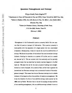
So far we have considered a general type of qubit. As an example of experimental implementation, let us now consider each qubit as a superconducting phase qubit. In reality, a third higher level |2⟩ for each phase qubit here needs to be considered during the operations described above, since this level |2⟩ may be occupied due to the |1⟩ ↔ |2⟩ transition induced by the cavity mode(s), which will turn out to affect the operation fidelity. Hence, to quantify how well the proposed protocol works out, we will analyze the fidelity of the operation for both entanglement generation and information transfer, by considering a third higher level |2⟩ . Since three levels are now involved, we rename the three qubits 1, 2, and A as qutrits 1, 2, and A, respectively. When the intercavity crosstalk coupling and the unwanted |1⟩ ↔ |2⟩ transition of each phase qutrit are considered, the Hamiltonian (1) is modified as follows e I = HI + HI′ , H
(16)
6
˄a˅
˄b˅ d~2
d~1 � g~1
�
�
g~2
d1 �
�
d2
�
�
�
g2
g1
�
�
�
�
˄c˅ d~A1 �
$
g~ A1
d~A2
g~A2
d A2
�
d A1
$
g A1
�
g A2
$
FIG. 2
FIG. 2: (Color online) Illustration of qutrit-cavity interaction. (a) Cavity 1 is dispersively coupled to the |0⟩ ↔ |1⟩ transition with coupling constant g1 and detuning δ1 , but far-off resonant (i.e., more detuned) with the |1⟩ ↔ |2⟩ transition of qutrit 1 with coupling consant ge1 and detuning δe1 . (b) Cavity 2 is dispersively coupled to the |0⟩ ↔ |1⟩ transition with coupling constant g2 and detuning δ2 , but far-off resonant with the |1⟩ ↔ |2⟩ transition of qutrit 2 with coupling consant ge2 and detuning δe2 . (c) Cavity 1 (cavity 2) dispersively interacts with the |0⟩ ↔ |1⟩ transition with coupling constant gA1 (gA2 ) and detuning δA1 (δA2 ), but is far-off resonant with the |1⟩ ↔ |2⟩ transition of qutrit A with coupling consant geA1 (e gA2 ) and detuning δeA1 (δeA2 ). Here, δj = ω10j − ωcj , δej = ω21j − ωcj , δAj = ω10A − ωcj , and δeAj = ω21A − ωcj (j = 1, 2), where ω10j (ω21j ) is the |0⟩ ↔ |1⟩ (|1⟩ ↔ |2⟩) transition frequency of qutrit j, ω10A (ω21A ) is the |0⟩ ↔ |1⟩ (|1⟩ ↔ |2⟩) transition frequency of qutrit A, and ωcj is the frequency of cavity j (j = 1, 2).
where HI is the needed interaction Hamiltonian given in Eq. (1) above, while HI′ is the unwanted interaction Hamiltonian, given by HI′ =
2 ∑
2 ( ) ∑ ( ) e e + + gej eiδj t aj σ21j + h.c. + geAj eiδAj t aj σ21A + h.c.
j=1
j=1
( ) +g12 ei∆t a1 a+ 2 + h.c. ,
(17)
+ + where σ21j = |2⟩j ⟨1| and σ21A = |2⟩A ⟨1| . The first term represents the unwanted off-resonant coupling between the
7
Fidelity F
0.98 0.96 g12 = 0 g12 = 0.2gA2 g12 = 0.4gA2 g12 = 0.6gA2 g12 = 0.8gA2
0.94 0.92 0.90 5
7
9
11
13
15
17
19
21
23
Detuning b FIG. 3: (Color online) Fidelity of the entanglement preparation versus the normalized detuning b = |δ1 | /g1 . Refer to the text for the parameters used in the numerical calculation.
mode of cavity j and the |1⟩ ↔ |2⟩ transition of qutrit j, with coupling constant gej and detuning δej = ω21j − ωcj [Fig. 2(a)], while the second term indicates the unwanted off-resonant coupling between the mode of cavity j and the |1⟩ ↔ |2⟩ transition of qutrit A, with coupling constant geAj and detuning δeAj = ω21A − ωcj [Fig. 2(b)]. It should be mentioned that the term describing the cavity-induced coherent |0⟩ ↔ |2⟩ transition for each qutrit is not included in the Hamiltonians HI′ , since this transition is negligible because of ωcj ≪ ω20j , ω20A (j = 1, 2) (Fig. 2). The last term describes the intercavity crosstalk betwee the two cavities, with ∆ = ωc2 − ωc1 = δA1 − δA2 . The dynamics of the lossy system, with finite qutrit relaxation and dephasing and photon lifetime included, is determined by 2 [ ] ∑ dρ eI , ρ + = −i H κj L [ˆ aj ] dt j=1 ∑ { [ ] [ − ] [ − ]} + γj L σj− + γ21j L σ21j + γ20j L σ20j j=1,2,A
+
∑
{γj,φ1 (σ11j ρσ11j − σ11j ρ/2 − ρσ11j /2)}
j=1,2,A
+
∑
{γj,φ2 (σ22j ρσ22j − σ22j ρ/2 − ρσ22j /2)} ,
(18)
j=1,2,A − − where σ20j = |0⟩j ⟨2| , σ20A = |0⟩A ⟨2| , σ11j = |1⟩j ⟨1| , σ22j = |2⟩j ⟨2| ; and L [Λ] = ΛρΛ+ − Λ+ Λρ/2 − ρΛ+ Λ/2,with − − − Λ=a ˆj , σj , σ21j , σ20j . In addition, κj is the photon decay rate of cavity aj , γj is the energy relaxation rate of the level |1⟩ of qutrit j, γ21j (γ20j ) is the energy relaxation rate of the level |2⟩ of qutrit j for the decay path |2⟩ → |1⟩ (|0⟩), and γj,φ1 (γj,φ2 ) is the dephasing rate of the level |1⟩ (|2⟩) of qutrit j. The fidelity of the operation is given by
F = ⟨ψid | ρe |ψid ⟩ ,
(19)
where |ψid ⟩ is the output state of an ideal system (i.e., without dissipation, dephasing, and crosstalks) as discussed in the previous section; and ρe is the final density operator of the system when the operation is performed in a realistic physical system. For entanglement preparation, |ψid ⟩ is |ϕ⟩ |0⟩c1 |0⟩c2 ; while for information transfer, it is the state |φ⟩ |0⟩c1 |0⟩c2 . Here and above, |0⟩cj is the vacuum state of cavity j (j = 1, 2).
8
√ FIG. 4: (Color online) Fidelity of the information transfer versus (b, α). Here, the detuning is b = |δ1 | /g1 , and α = 1 − β 2 . For simplicity, here we consider the transferred state α |0⟩ + β |1⟩, with real numbers α and β. For the parameters used in the numerical calculation, see the text.
A.
Fidelity for the entanglement preparation
Without loss of generality, let us consider three identical superconducting phase qutrits. According to the condition (4), we set δ1 / (2π) = δA1 / (2π) = −0.5 GHz and δ2 / (2π) = δA2 / (2π) = −1 GHz. For the setting here, we have ∆/2π = 0.5 GHz. Set δej = δj − 0.05ω10j and δeAj = δAj − 0.05ω10A (j = 1, 2) [49]. For superconducting phase qubits, the typical qubit transition frequency is between 4 and 10 GHz. Thus, we choose ω10A /2π, ω10j /2π ∼ 6.5 GHz. Note that g2 is determined based on Eq. (10), given δ1 , δ2 , and g1 ; and thus the ratio of δ2 /g2 can be calculated, if δ2√and g2 are known. δ1 and δ2 . Next, one has gej ∼ 2gj √ In addition, gA1 and gA2 are determined based on Eq. (10), given −1 −1 and geAj ∼ 2gAj (j = 1, 2) for the phase qubit here. For example, we choose γj,φ1 = γj,φ2 = 2.5 µs, γj−1 = 10 µs, −1 −1 −1 γ21j = 7.5 µs, and γ20j = 30 µs; and κ−1 1 = κ2 = 5 µs. For a phase qutrit with the three levels considered here, the |0⟩ ↔ |2⟩ dipole matrix element is much smaller than that of the |0⟩ ↔ |1⟩ and |1⟩ ↔ |2⟩ transitions. Thus, −1 −1 −1 γ20j ≫ γ10j , γ21j . For the parameters chosen above, the fidelity versus b = |δ1 | /g1 is plotted in Fig. 3 for g12 = 0, 0.2gmax , 0.4gmax , 0.6gmax , 0.8gmax . From Fig. 3, one can see that for g12 ≤ 0.2gmax , the effect of intercavity cross coupling between the two cavities on the fidelity of the operation is negligible, which can be seen by comparing the top two curves. Moreover, Fig. 3 shows that for b ∼ 11 and g12 = 0.2gmax , a high fidelity ∼ 98% is available for the entanglement preparation.
B.
Fidelity for the information transfer
The parameters used in the numerical calculation are the same as above. Fig. 4 shows the fidelity versus (b, α), which is plotted for g12 = 0.2gmax . One can see from Fig. 4 that for b ∼ 9, a high fidelity > 97% is achievable for the information transfer. Further, it is predicted that a higher fidelity can be obtained when g12 < 0.2gmax . This condition, g12 ≤ 0.2gmax , is not difficult to satisfy with the typical capacitive cavity-qutrit coupling illustrated in Fig. 1(a). As long as the cavities are physically well separated, the intercavity cross-talk coupling strength is g12 ∼ gA1 C2 /CΣ , gA2 C1 /CΣ , where CΣ = C1 + C2 + Cq . For C1 , C2 ∼ 1 fF and CΣ ∼ 102 fF (the typical values of the cavity-qutrit coupling capacitance and the sum of all coupling capacitance and qutrit self-capacitance, respectively), we have g12 ∼ 0.01gA1 , 0.01gA2 . Note that gAj ≤ gmax . Thus, the condition g12 ≤ 0.2gmax can be readily met in experiments. Hence, implementing designs with sufficiently weak direct intercavity couplings is straightforward. For b ∼ 11, we have {g1 , g2 , gA1 , gA2 } ∼ {45.5, 64.3, 32.2, 45.5} MHz. Note that a coupling constant ∼ 220 MHz can be reached for a superconducting qutrit coupled to a one-dimensional CPW (coplanar waveguide) resonator [35], and that T1 and T2 can be made to be on ′the order of 10 − 100 µs or longer for state-of-the-art superconducting devices [50]. The energy relaxation time dephasing time T2′ of the level |2⟩ are comparable to T1 and T2 , √ T1 and ′ ′ respectively. For instance, T1 ∼ T1 / 2 and T2 ∼ T2 for phase qutrits. For ω10A /2π, ω10j /2π ∼ 6.5 GHz chosen
9 above, we have ωc1 /2π ∼ 6 GHz and ωc2 /2π ∼ 5.5 GHz. For the cavity frequencies chosen here and the values of −1 κ−1 used in the numerical calculation, the required quality factors for the two cavities are Q1 ∼ 1.9 × 10⁵ 1 and κ2 and Q2 ∼ 1.7 × 10⁵ , respectively. Note that superconducting CPW resonators with a loaded quality factor Q ∼ 106 have been experimentally demonstrated [51,52], and planar superconducting resonators with internal quality factors above one million (Q > 106 ) have also been recently reported [53]. Our analysis given here demonstrates that highfidelity implementation of the entangled state and the information transfer by using this proposal is feasible within the present circuit QED technique. We remark that further investigation is needed for each particular experimental setup. However, this requires a rather lengthy and complex analysis, which is beyond the scope of this theoretical work. IV.
CONCLUSION
We have proposed a method to generate quantum entanglement and perform quantum information transfer between two spatially-separate superconducting qubits residing in two different cavities. As shown above, this work is of interest because the entanglement generation and information transfer implementation do not require employing photons of the cavities as quantum buses and thus decoherence caused due to the cavity decay is greatly supressed during the entire operation. The proposal does not require applying classical microwave pulses and needs only one step of operation and one superconducting coupler qubit, so that the circuit complexity is much reduced and the operation is greatly simplified. In addition, our analysis shows that high-fidelity implementation of this proposal with superconducting phase qubits is feasible within the present circuit QED technology. Finally, it is noted that the method presented here is quite general, and can be applied to accomplish the same task with the coupler qubit replaced by a different type of qubit such as a quantum dot, or with the two intercavity qubits replaced by other two qubits, e.g., two atoms, two quantum dots, two NV centers, and so on. ACKNOWLEDGMENTS We thank Shi-Biao Zheng for many fruitful discussions. C.P.Y. was supported in part by the National Natural Science Foundation of China under Grant No. 11074062, the Zhejiang Natural Science Foundation under Grant No. LZ13A040002, and the funds from Hangzhou Normal University under Grant No. HSQK0081. Q.P.S. was supported by the National Natural Science Foundation of China under Grant No. 11147186. This work is also partially supported by the ARO, RIKEN iTHES Project, MURI Center for Dynamic Magneto-Optics, JSPS-RFBR contract No. 12-0292100, Grant-in-Aid for Scientific Research (S), MEXT Kakenhi on Quantum Cybernetics, and the JSPS via its FIRST program.
[1] [2] [3] [4] [5] [6] [7] [8] [9] [10]
[11] [12] [13] [14] [15] [16] [17]
Cirac J I and Zoller P 1995 Phys. Rev. Lett. 74 4091 Blatt R and Wineland D 2008 Nature 453 1008 Duan L M, Lukin M D, Cirac J I and Zoller P 2001 Nature 414 413 Chou C W, Laurat J, Deng H, Choi K S, Riedmatten H D, Felinto D, and Kimble H J 2007 Science 316 1316 Mabuchi H and Doherty A C 2002 Science 298 1372 Hagley E, Maˆıtre X, Nogues G, Wunderlich C, Brune M, Raimond J M, and Haroche S 1997 Phys. Rev. Lett. 79 1 Zheng S B and Guo G C 2000 Phys. Rev. Lett. 85 2392 Osnaghi S, Bertet P, Auffeves A, Maioli P, Brune M, Raimond J M, and Haroche S et al. 2001 Phys. Rev. Lett. 87 037902 Cirac J I, Zoller P, Kimble H J, and Mabuchi H 1997 Phys. Rev. Lett. 78 3221; Pellizzari T 1997 Phys. Rev. Lett. 79 5242 Ye S Y, Zhong Z R, and Zheng S B 2008 Phys. Rev. A 77 014303; Serafini A, Mancini S, and Bose S 2006 Phys. Rev. Lett. 96 010503; Yin Z Q and Li F L 2007 Phys. Rev. A 75 012324; L¨ u X Y, Liu J B, Ding C L, and Li J H 2008 Phys. Rev. A 78 032305; L¨ u X Y, Song P J, Liu J B, and Yang X 2009 Opt. Express 17 14298; Dong Y L, Zhu S Q, and You W L 2012 Phys. Rev. A bf 85 023833 Ritter S, N¨ olleke C, Hahn C, Reiserer A, Neuzner A, Uphoff M, M¨ ucke M, Figueroa E, Bochmann J, and Rempe G 2012 Nature 484 195 You J Q and Nori F 2005 Physics Today 58 (11) 42; You J Q and Nori F 2011 Nature 474 589 Xiang Z L, Ashhab S, You J Q, and Nori F 2013 Rev. Mod. Phys. 85 623 Buluta I, Ashhab S, and Nori F 2011 Reports on Progress in Physics 74 104401; Shevchenko S N, Ashhab S, and Nori F 2010 Phys. Reports 492 1; Nation P D, Johansson J R, Blencowe M P, and Nori F 2012 Rev. Mod. Phys. 84 1 Wallraff A, Schuster D I, Blais A, Frunzio L, Huang R S, Majer J, Kumar S, Girvin S M, and Schoelkopf R J 2004 Nature 431 162 Houck A A et al. 2007 Nature 449 328 Marquardt F and Bruder C 2001 Phys. Rev. B 63 054514
10 [18] Liu Y X, Wei L F, and Nori F 2004 Europhys. Lett. 67 941 [19] Marquardt F 2007 Phys. Rev. B 76 205416 [20] Mariantoni M, Storcz M J, Wilhelm F K, Oliver W D, Emmert A, Marx A, Gross R, Christ H, and Solano E arXiv:condmat/0509737. [21] Hofheinz M, Weig E M, Ansmann M, Bialczak R C, Lucero E, Neeley M, OConnell A D, Wang H, Martinis J M, and Cleland A N 2008 Nature 454 310; Wang H, Hofheinz M, Ansmann M, Bialczak R C, Lucero E, Neeley M, OConnell A D, Sank D, Wenner J, Cleland A N, and Martinis J M 2008 Phys. Rev. Lett. 101 240401 [22] Hofheinz M, Wang H, Ansmann M, Bialczak R C, Lucero E, Neeley M, O’Connell A D, Sank D, Wenner J, Martinis J M, and Cleland A N 2009 Nature 459 546 [23] Yang C P, Chu S I, and Han S 2003 Phys. Rev. A 67 042311 [24] You J Q and Nori F 2003 Phys. Rev. B 68 064509 [25] Blais A, Huang R S, Wallraff A, Girvin S M, and Schoelkopf R J 2004 Phys. Rev. A 69 062320 [26] Yang C P, Chu S I, and Han S 2004 Phys. Rev. Lett. 92 117902 [27] Plastina F and Falci G 2003 Phys. Rev. B 67 224514 [28] Blais A, Maassen van den Brink A, and Zagoskin A M 2003 Phys. Rev. Lett. 90 127901 [29] Helmer F and Marquardt F 2009 Phys. Rev. A 79 052328 [30] Bishop L S et al. 2009 New J. Phys. 11 073040 [31] Yang C P, Liu Y X, and Nori F 2010 Phys. Rev. A 81 062323 [32] Yang C P, Zheng S B, and Nori F 2010 Phys. Rev. A 82 062326 [33] Majer J et al. 2007 Nature 449 443 [34] Leek P J, Filipp S, Maurer P, Baur M, Bianchetti R, Fink J M, Goppl M, Steffen L, and Wallraff A 2009 Phys. Rev. B 79 180511(R) [35] DiCarlo L et al. 2010 Nature 467 574 [36] Mariantoni M et al. 2011 Science 334 61 [37] Fedorov A, Steffen L, Baur M, Silva M P, and Wallraff A 2012 Nature 481 170 [38] Mariantoni M, Deppe F, Marx A, Gross R, Wilhelm F K, and Solano E 2008 Phys. Rev. B 78 104508 [39] Strauch F W, Jacobs K, and Simmonds R W 2010 Phys. Rev. Lett. 105 050501 [40] Merkel S T and Wilhelm F K 2010 New J. Phys. 12 093036 [41] Wang H et al. 2011 Phys. Rev. Lett. 106 060401 [42] Yang C P, Su Q P, and Han S 2012 Phys. Rev. A 86 022329 [43] Yang C P, Su Q P, Zheng S B, and Han S 2013 Phys. Rev. A 87 022320 [44] Zheng Z F, Su Q P, and Yang C P 2013 J. Phys. Soc. Jpn. 82 084801 [45] Zheng S B 2011 Phys. Rev. Lett. 87 230404 [46] Clarke J and Wilhelm F K 2008 Nature 453 1031 [47] Neeley M, Ansmann M, Bialczak R C, Hofheinz M, Katz N, Lucero E, OConnell A, Wang H, Cleland A N, and Martinis J M 2008 Nature Phys. 4 523; Zagoskin A M, Ashhab S, Johansson J R, and Nori F 2006 Phys. Rev. Lett. 97 077001 [48] Sandberg M, Wilson C M, Persson F, Bauch T, Johansson G, Shumeiko V, Duty T, and Delsing P 2008 Appl. Phys. Lett. 92 203501 [49] For a phase qutrit, a ratio 5% of the anharmonicity between the |0⟩ ↔ |1⟩ transition frequency and the |1⟩ ↔ |2⟩ transition frequency to the the |1⟩ ↔ |2⟩ transition frequency is readily achieved in experiments. [50] see, Bylander J et al. 2011 Nature Phys. 7 565; Paik H 2011 Phys. Rev. Lett. 107 240501; Chow J M et al. 2012 Phys. Rev. Lett. 109 060501; Rigetti C et al. 2012 Phys. Rev. B 86 100506(R); R. Barends et al., arXiv:1304.2322 [51] Chen W, Bennett D A, Patel V, and Lukens J E 2008 Supercond. Sci. Technol. 21 075013 [52] Leek P J, Baur M, Fink J M, Bianchetti R, Steffen L, Filipp S, and Wallraff A 2010 Phys. Rev. Lett. 104 100504 [53] Megrant A et al. 2012 Appl. Phys. Lett. 100 113510