We combine the entropy terms of model (eq. (2)) and training textures (eq. .... into the models, additional landmark points outside the objects were defined. In.
Entropy-Optimized Texture Models Sebastian Zambal, Katja B¨ uhler, and Jiˇr´ı Hlad˚ uvka VRVis Research Center for Virtual Reality and Visualization http://www.vrvis.at
Abstract. In order to robustly match a statistical model of shape and appearance (e.g. AAM) to an unseen image it is crucial to employ a robust measure of how well the model fits. Dense sampling of texture over the region covered by the shape of interest makes comparison of model and image in principle robust. However, when merely texture differences are taken into account, problems with low contrast regions, fuzzy features, global intensity variations, and irregularly varying structures occur. In this paper we introduce a novel entropy-optimized texture model (ETM). We map gray values of training images such that pixels represent anatomical structures optimally in terms of information entropy. We match the ETM to unseen images employing Bayes’ law. We validate our approach using four training sets (hearts in basal region, hearts in mid region, brain ventricles, and lumbar vertebrae) and conclude that ETMs perform better than AAMs. Not only they reduce the average point-to-contour error, they are better suited to cope with large texture variances due to different scanners and even modalities.
1
Introduction
Statistical shape models exploit prior knowledge of shape to perform robust segmentation. Active Shape Models (ASMs) [1] are based on Principal Component Analysis (PCA) of a set of corresponding training shapes. In the matching process the model is attracted by image features (e.g. edges) and iteratively deformed accordingly. Additionally to shape Active Appearance Models (AAMs) [2] incorporate texture. As for shape, PCA is used to represent statistical texture variation. In the following we motivate our new approach to texture representation for statistical models by resuming some critical aspects of texture modeling in AAMs. Model matching is understood as finding the model instance which exhibits the minimal difference to the unseen image. Hence it is very important to employ an effective difference measure which consistently reflects how well a given model instance matches the image. In the context of AAMs typically a measure based on texture differences is used. The assumption is made that large texture differences correspond to large misalignment of the model. However, it may happen that clearly separable structures exhibit low contrast (e.g. lung and myocardium in cardiac MRI) and a misalignment does not lead to large texture
differences. On the other hand, regions showing fuzzy anatomical structures (e.g. papillary muscles, trabeculae of the heart, trabeculae of spongy bone) may lead to very large texture differences which may not necessarily correspond to a large misalignment. With texture difference based objective functions it might thus happen, that regions of low contrast are over-ruled by regions showing fuzzy structures. For many data sets we observed that a large number of PCA texture parameters are required to sufficiently well cover variations in a training set. For the examples we investigated in this paper we observed that typically the sorted eigenvalues of shape decrease much faster than those of texture. This suggests that PCA is not the optimal choice for texture modeling. To improve the quality of AAMs, a texture normalization step is usually applied before statistical analysis. The goal is to keep irrelevant texture variations (e.g. global variations in brightness or gamma) out of the model. In the scope of AAMs different methods have been proposed (e.g. different types of non-linear texture normalization [3]). However, in general it is hard to predict which type of texture normalization will lead to good results for which kind of data. A very popular matching criterion for medical image registration is mutual information (MI) [4]. The great advantage of this measure is that it even enables registration of images acquired using different imaging methods. Mutual information is based on entropy terms and in its original form limited to registration of a pair of images. Thus, although it would be reasonable to integrate mutual information into the AAM framework this can not be done straight forwardly. Bayesian reasoning makes use of posterior probabilities to quantify how well some model explains unknown data. Based on Bayes’ law prior probability is combined with the likelihood of an observation to derive a posterior probability of a model. Bayesian reasoning has a sound mathematical background and is wellestablished for pattern recognition tasks. Thus it seems worth to incorporate it into the framework of statistical models of shape and appearance. To tackle the above issues we borrow ideas about entropy from groupwise registration and formulate a novel probabilistic texture model. In section 2 we derive an optimization function for texture normalization which has similarities with a recently proposed function for shape correspondence optimization [5]. In section 3 we match the model to unseen images using Bayesian inference. We demonstrate the robustness of our entropy-optimized texture model (ETM) on four different 2D training sets: vertebra, brain ventricles, mid cardiac, and basal cardiac slices (section 4). Based on this validation we conclude in section 5 that the proposed ETM outperforms AAMs and even copes with texture variations due to different imaging modalities (different MRI scanners, T1/T2/FLAIR, CT/MRI).
Fig. 1. The entropy texture model: the normalized corresponding pixels are modeled by probability distributions.
2
Entropy texture model: construction
Similar to AAM, the input for the model we propose is a set of m training images Ti , annotated with a fixed number of landmark points in correspondence, consistently triangulated, resampled by n texels and quantized to ri gray levels: While similar in shape description by mean and principal components, our model differs from the AAM in the representation of texture. Each of the n model texels tj captures the statistical variations observed at corresponding training pixels. In order to keep unspecific intensity variations out of the model we propose to normalize the training images using generic intensity mappings. The task is to optimize m intensity maps fi that quantize the training images from ri to s gray levels. fi : Zri → Zs , s � ri i = 1...m (1) In the following we design the cost function to assess mappings fi . Each model’s texel tj observes m occurrences of the s possible mapped gray values at corresponding training texels. Such a set of observations can be interpreted as probability density function (PDF) and we denote it pj . pj (gk0 ) is the probability that at corresponding texel tj a mapped gray value gk0 is observed. The predictability of mapped gray values expressed by PDFs varies across model texels. Figure 1 illustrates the situation for two texels. While PDF p2 exhibits a single high peak, p10 is rather equally distributed. This suggests that predictions of gray values for texel t2 will be more reliable than for texel t10 . Inspired by Balci et al. [6] we propose to favor reliability (similar to p2 ) and to penalize uncertainty (similar to p10 ) by minimizing the entropy of the Ps according PDFs: H(pj ) = − k=1 pj (gk0 ) log2 (pj (gk0 )). Considering all n model texels yields a cost function that measures the quality of mappings fi : n
H
model
1X = H(pj ) n j=1
→ min
(2)
H model yields minimum when all mapped training images degenerate to a single gray value. In this case the model only allows a single gray value to be observed and thus exhibits maximal specificity.
T1
T2
T3
f1 (T1 )
(a) original
f2 (T2 )
f3 (T3 )
(b) optimized
Fig. 2. A sample training set (two different MRI scanners and a CT) before (a) and after (b) mapping to three gray levels (s = 3).
However, this specificity has to be regarded in relation to the training images which contain no information once degenerated. This motivates for a compensation term which drives the mapped training textures fi (Ti ) towards maximal information content. We measure the information content by image entropy H(fi (Ti )) and aim at its maximization across the entire normalized training set: m
H
tex
1 X = H(fi (Ti )) m i=1
→ max
(3)
H tex is maximal when the texture transforms fi maximize the information content of the textures Ti . This is equivalent to histogram equalization. We combine the entropy terms of model (eq. (2)) and training textures (eq. (3)) with the goal to maximize: H tex − H model
→ max
(4)
There is no need for an ad-hoc weighting of the two terms since they are commensurate, i.e., measured in bits per texel. An objective function similar to (4) has recently been proposed for shape correspondence optimization [5]. In this work similarly two energy terms are used: one for individual shapes and one for a shape ensemble. This makes our entropy-optimization of texture a direct analogy to Minimal Description Length (MDL) of shape with the difference that we do not stick to Gaussian distribution as description language for texture. We used Simulated Annealing to optimize mappings fi subject to the cost function (4). Represented by lookup tables, the texture mappings fi are initialized to linearly remap the training images to s levels. During optimization the lookup tables are updated in each iteration. After optimization the mapped training textures represent structures with minimal uncertainty at maximum information content (figure 2(b)). Figure 3 shows entropies of the optimized distributions of four models we use for validation in section 4. While bright texels exhibit strong variations (high entropy), dark texels represent high predictability (low entropy).
(a) heart LV+RV
(b) heart LV
(c) vertebra
(d) brain ventricles
Fig. 3. Entropy (brightness) of model PDFs after optimization.
3
Entropy texture model: matching
In contrast to AAMs, the entropy model we just built has only shape parameters: position, scale, rotation, and a vector of parameters identical to ASM. In this section we describe how the model is matched to an unseen image by iteratively changing its shape parameters. The cost function that quantifies a particular shape instance S involves model PDFs and the unseen texture U = (u1 , . . . , un ) overlapped by the model. In every iteration the cost is computed in two steps. Mapping of the unseen’s texture As our model texels capture PDFs of the s gray values we first need to normalize U accordingly: we seek for a function fu : Zru → Zs that maps the unseen to s gray levels. We want to find a suitable intensity mapping for each of the ru gray values. For a fixed gray value u ˆ all model texels observing it vote according to their PDFs: out of the s possibilities the target gray value leading to the maximal likelihood is assigned. Formally: Y fu (ˆ u) = argmax pj (gk0 ) k = 1...s (5) 0 gk
uj =ˆ u
Cost function To assess how well the shape instance S fits to the unseen image, we compare model PDFs p(.) to the normalized texels U 0 = fu (U ) = {fu (uj )}nj=1 . To convey this we consider maximizing the posterior probability P (S|U 0 ) of the shape instance S given the observed normalized texture U 0 . According to Bayes’ law [7] the posterior is proportional to the product of a likelihood and a prior. The likelihood P (U 0 |S) of the observed normalized texture U 0 given the shape instance S is (under the naive Bayesian assumption) the product of probabilities of the normalized texels. The prior probability P (S) of shape instance S is calculated feeding its parameters into the multivariate Gauss distribution that corresponds to the PCA shape space (please refer to [7] for details). Putting both terms together yields the cost function: n Y p(S|U 0 ) ∝ p(U 0 |S) p(S) = pj (fu (uj )) p(S) (6) j=1
(a)
(b)
(c)
(d)
(e)
Fig. 4. Matching of a model comprising five target values (s = 5): original image with initialized contour (a), maximum likelihood estimate for fu for initial contour (b), after 4 iterations (c), and after 8 iterations (d). Final match over the original unseen (e).
Strategy and implementation issues In contrast to AAM there are no texture parameters to optimize. The search space is only spanned by shape parameters and typically has not more than 10 to 15 dimensions. This fact makes exhaustive search strategies similar to [8] affordable and we employ such a scheme in this work. Figure 4 illustrates how a model with five gray levels evolves during matching. Shape and maximum likelihood texture mapping converge consistently. Any pj (.) being zero degenerates the equations (5) and (6). In order to avoid this we assign a small compensation probability of 1/(2m) and renormalize the distribution pj . To avoid numerical instability due to the large number of multiplications in (5) and (6) we maximize sums of logarithms of the probabilities instead.
4
Validation and results
In order to validate our approach we compared the segmentations achieved by ETM (s = 5) to those achieved by standard AAM. For cross validation we split training sets into reasonable subsets (e.g. images from same patient or same scanner). Every image was matched as an unseen by a model built from complementary subsets. Model matching was performed by initializing each of the models close to the correct contours (hence no automatic initialization of the model was done). Matching accuracy was measured in terms of average point-tocontour distances. To include enough information about object boundary regions into the models, additional landmark points outside the objects were defined. In the following we describe the data sets and the results in details. Heart LV+RV, basal region: contains short axis slices from the base of the heart showing few or no papillary muscles. The training set comprises data from four different sources: CT and three different MR protocols. Annotations define the contours of inner and outer boundaries of the left ventricle (LV) and the inner contour of the right ventricle (RV). ETM performed better in 23 out of 38 cases, reducing the average point-to-contour distance from 4.36 to 3.36 mm. Heart LV, mid region: includes 42 short axis MR images from the mid region of the heart exhibiting large texture variations due to papillary muscles.
Images stem from two different MR scanners.The average pixel size is 1.39mm. Annotations define the contours of the inner and outer boundaries of the left ventricle (LV). ETM performed better in 38 out of 42 cases, reducing the average point-to-contour distance from 4.02 to 2.38 mm. Brain ventricle: comprises 17 transversal MR slices of 15 different patients. One patient is represented by a T1 image and a FLAIR image. Another patient is represented by a T2 image and a FLAIR image. Remaining patients are represented each by a T1 image. The average pixel size is 0.85mm. Annotations define the contours of brain ventricles. ETM performed better in 16 out of 17 cases, reducing the average point-to-contour distance from 3.53 to 1.67 mm. Vertebra: consists of 13 CT slices from 4 different patients showing transversal sections of lumbar vertebrae. The average pixel size is 0.32mm. Annotations define the outer contour of the vertebra and the contour of the spinal canal. ETM performed better in 9 out of 13 cases, reducing the average point-to-contour distance from 2.67 to 2.06 mm. On average our ETMs clearly outperformed AAMs. Results are summarized graphically in figure 5.
5
Conclusions and future work
We proposed a novel texture model for medical image segmentation. Its texture is described by probability distributions of individual texels. Moreover, these probabilities are optimized by information entropy terms. This allows to effectively cope with unspecific intensity variations in the training set caused e.g. by different modalities, scanner settings, and fuzzy anatomical structures. The model is matched to unseens in accordance to Bayesian reasoning. There are two major messages we would like to conclude with. First, ETM perform better than AAM, as it is shown in the validation. Second, thanks to intensity normalizations that are integral part of model construction, some requirements on training texture (e.g. Gaussian distribution) can be relaxed. We have demonstrated this with training sets containing mixtures of CT/MR and MR T1/T2/FLAIR images. There are several issues left for future work. To name a few, we intend to address extension to 3D volume textures, automatic initialization, and acceleration of the matching in near future.
References 1. Cootes, T.F., Taylor, C.J., Cooper, D.H., Graham, J.: Active Shape Models – Their training and application. Computer Vision and Image Understanding 61(1) (1995) 38–59 2. Cootes, T.F., Edwards, G.J., Taylor, C.J.: Active Appearance Models. In: European Conference on Computer Vision. Volume 2. (1998) 484–498 3. Kittipanya-ngam, P., Cootes, T.F.: The effect of texture representations on AAM performance. In: International Conference of Pattern Recognition. (2006) 328–331
4. Viola, P., Wells, W.M.: Alignment by maximization of Mutual Information. International Journal of Computer Vision 24(2) (1997) 137–154 5. Cates, J., Fletcher, P.T., Styner, M., Shenton, M., Whitaker, R.: Shape modeling and analysis with entropy-based particle systems. In: Information Processing in Medical Imaging. (2007) 333–345 6. Balci, S.K., Golland, P., Shenton, M., Wells, W.M.: Free-form B-spline deformation model for groupwise registration. In: Medical Image Computing and Computer– Assisted Intervention (Statistical Registration Workshop). (2007) 23–30 7. Bishop, C.M.: Pattern Recognition and Machine Learning. Springer (2006) 8. de Bruijne, M., Nielsen, M.: Shape particle filtering for image segmentation. In: Medical Image Computing and Computer–Assisted Intervention. Volume 1. (2004) 168–175
vertebra
heart LV in mid region
Fig. 5. Average point-to-contour errors [mm] achieved by ETMs and AAMs. Example thumbnails show final segmentations.
brain ventricles
heart LV+RV in basal region