Environmental Data Mining and Modelling Based on Machine Learning Algorithms and Geostatistics M. Kanevskia, R. Parkinb, A. Pozdnukhovb, V. Timoninb, M. Maignanc, B. Yatsalod, S. Canue a
b
IDIAP Dalle Molle Institute for Perceptual Artificial Intelligence, Simplon 4, 1920 Martigny, Switzerland, (
[email protected])
IBRAE Nuclear Safety Institute, Russian Academy of Sciences, 113191 Moscow, Russia (
[email protected]) c
Lausanne University, Lausanne, Switzerland d
OINPE Institute, Obninsk, Russia e
INSA, Rouen, France
Abstract: The paper presents some contemporary approaches to the spatial environmental data analysis, processing and presentation. The main topics are concentrated on the decision–oriented problems of environmental and pollution spatial data mining and modelling: valorisation and representativity of data with the help of exploratory data analysis, topological, statistical and fractal measures of monitoring networks, spatial predictions and classifications, probabilistic and risk mapping, development and application of conditional stochastic simulation models. The set of tools used consists of machine learning algorithms (MLA) – Multilayer Perceptron, General Regression Neural Networks, Probabilistic Neural Networks, Radial Basis Function Networks, Support Vector Machines and Support Vector Regression, and recently developed geostatistical predictive and simulation models. The innovative part of the report deals with integrated/hybrid models, including ML Residuals Kriging/Cokriging predictions, ML Residuals Simulated Annealing/Sequential Gaussian simulations. The objective of the integrated models is twofold: from one side ML algorithms efficiently solve problems of spatial non-stationarity, which are difficult for geostatistical approach; from another side geostatistical tools are widely and successfully applied to characterise the performance of the ML algorithms, analysing the quality and quantity of the spatially structured information extracted from data by ML. Moreover, mixture of ML data driven and geostatistical model based approaches are attractive for decision-making process. Keywords: environmental data mining and assimilation, geostatistics, machine learning 1.
other facts complicate analysis, processing and interpretation of the results. Usually it is supposed that data can be decomposed into two parts: Z(x)=M(x)+e(x), where M(x) represents large scale deterministic variations (trends), and e(x) represents small scale stochastic variations. Geostatistical approach offers several possible models in case of spatial trends (spatial nonstationarity): universal kriging, residual kriging, moving window regression residual kriging, science-based approaches, etc. These approaches have been considered by Cressie [1991], Deutsch et al. [1992], Dowd [1994], Neuman et al. [1984], Gambolati et al. [1987] and Haas [1996]. Each of
INTRODUCTION
Most environmental data represent a combination of several spatial phenomena of different origin and appear as the complex spatial patterns at different scales. In some cases the original observations are taken with significant measurement errors and may contain a number of outliers. Spatial trends reproducing large-scale processes complicate variography – a basic geostatistical tool, describing spatial correlations, and sometimes make difficult or impossible developing of a valid variogram model. These and
414
these methods has its own advantages and drawbacks.
nonparametric, robust model for the large scale non-linear structures (detrending) and then to use geostatistical models for the analysis of residuals modelling of small scale structured variations. Lets look more closely into the original ML Residual Simulations.
The present work is an extension (development of Neural Network Residuals Sequential Gaussian simulations (NNRSGS)) of the ideas presented by Kanevsky et al. [1996], where hybrid model – Neural Network Residuals Kriging (NNRK) – has been presented for the first time. The basic idea is to use feedforward neural network (FFNN), which is a well-known global universal approximator to model large-scale nonlinear trends, and then to use geostatistical interpolators/simulators for the residuals.
1. The data is prepared for the analysis: split into training and validation set, checked for outliers, analysed with variography tools. If ANN is used at the first step, the data is scaled on the interval [0.1, 0.9] to facilitate the training procedure. 2. Further ML algorithm is applied. Without loss of generality, in the present study Multilayer Perceptron (MLP) and Support Vector Regression are used. They are well known function approximators. The consideration of these algorithms for application in ML Residual Simulations is presented below. Accuracy test is MLA estimation at training points. It shows how well the MLA has been trained. Validation procedure – when MLA estimates values at validation points, which have not been used for training, – is a test of overall MLA performance, its ability to generalise and is especially used to avoid overtraining.
One of the principal advantages of ML algorithms is their ability to discover patterns in data, which are so obscure as to be imperceptible to human researches and standard statistical methods; the data exhibit significant unpredictable nonlinearity. Containing no data behaviour model, MLA depends only on the input data and the inner structure of the model, e.g. number of neurones, hidden layers, types of connections, information flow direction. MLA, depending on its architecture, can capture spatial peculiarities of the pattern at different scales describing both linear and non-linear effects. The performances of MLA are based on solid theoretical foundations. The objective of the integrated models developed in the current paper is twofold: from one side MLA efficiently solve problems of spatial nonstationarity, which are difficult for geostatistical approach; from another side geostatistical tools are widely and successfully applied to characterise the performance of the MLA by analysing the quality and quantity of the spatially structured information extracted from data. Moreover, mixture of ML data driven and geostatistical model based approaches are attractive for decision-making process because of their interpretability. The real case study on soil pollution is considered in detail: Chernobyl fallout – large-scale contamination of environment by radiologically important radionuclides. Details of the data can be found in Kanevski et al [1996].
2.
3. Accuracy test provides MLA residuals (estimated - measured) which are the base of the further analysis. Two cases are possible: • residuals are not correlated with the measurements, which means, that ANN has modelled all spatial structures represented in the raw data; • residuals show some correlation with the samples, than further analysis must be performed on the residuals to model this correlation. The remaining spatial correlation represents shortrange correlation structures. Long-range correlation (trend) in the whole area beyond the hot spots is very well modelled by MLA. 4. MLA residuals are explored using variography tools. Normal score transformation is performed to prepare data for further Gaussian simulations.
MACHINE LEARNING RESIDUAL GAUSSIAN SIMULATIONS
5. Sequential Gaussian simulation is applied to the MLA residuals. The idea of stochastic simulation is to develop a spatial Monte Carlo model/generator that will be able to generate many, in some sense equally probable, realisations of the random function (in general, described by joint probability density
The present work deals with an important development of hybrid MLA+geostat models firstly presented by Kanevsky et al. [1996] towards probabilistic/risk mapping. In short, the basic idea is to use MLA to develop a
415
Variogram analysis of normal score data discovered long-range structures (50 km) and local correlation (10-15 km) (see Figure 1 and 2). This conclusion leads to MLA use for trend modelling. Another problem with not de-trended data is that normal score variogram does not reach the sill=1, which is required for normally distributed variable.
function). Any realisation of the random function is called a nonconditional simulation. Realisations that honour the data are called conditional simulations. Basically, the simulations are trying to reproduce first (univariate distributions) and second moment (variograms). The realisations are determined by the conditional data, simulation model and random seed. The similarities and dissimilarities between realisations describe spatial variability and uncertainty. Simulations bring valuable information for the decision-oriented mapping of pollution. Postprocessing of simulations gives rise to probabilistic maps: maps of probabilities to be above/below some predefined decision levels. Gaussian random function models are widely used in statistics and simulations due to their analytical simplicity, they are well understood, and they are limit distributions of many theoretical results. They were successfully applied in many cases. In this work we shall use algorithm known as a Sequential Gaussian Simulations. Details on the models description and on the implemented algorithm can be found in Deutsch and Journel [1992].
Figure 1. Raw directional variograms for normal score CS137 samples.
6. Simulation value of the residuals appears after back normal transformation. Final ML Residual Simulations value is a sum of MLA estimate and sequential Gaussian simulation value of the residuals.
3.
Figure 2. Raw variogram rose for normal score CS137 samples. In the present study the MLP models with the following was used: 2 input neurons, describing spatial co-ordinates (X, Y); one or two hidden layers; output neuron describing Cs137 contamination. An important step deals with training and testing of the network. Backpropagation training with conjugate gradient, steepest descent, Levenberg-Marquardt, simulated annealing and genetic optimisation algorithms in order to avoid local minima were used. The trained network has been evaluated by using crossvalidation, and accuracy tests - prediction of the training data set with trained ANN. Accuracy test is used as a simple test describing how ANN captured the correlation between locations and contamination. The network has been validated by using independent data set. Then ANN is used for Cs137 spatial predictions/generalisations mapping. Result for the Cs137 ANN large scale mapping is presented in Figure 3.
CASE STUDY
Radioactive soil contamination caused by the Chernobyl fallout feature anisotropic highly variable and spotty spatial pattern. The multi-scale character of the pattern is due to numerous influencing factors. Structural analysis of sample data discovers limitation for use of stationary estimation/simulation models, like kriging or stochastic simulation. Exploratory spatial data analysis deals with the following steps: statistical analysis, spatial moving window statistics and trend analysis. This is an important phase of the study both for the MLA and geostatistical analyses. The basic statistical parameters of the Chernobyl data are following: minimum value Cs137=5.9, mean value Cs137=571.8, maximum value Cs137=4333.9, variance Cs137=315372, skewness Cs137=2.7 and kurtosis Cs137=16.9. As usually environmental data are positively skewed and their distributions are far from normal. Concentrations are measured in kBq/m2.
This result was obtained by using 5 hidden neurones respectively. It is evident that ANN has learned non-linear trends and that small-scale variations have been ignored. By using more
416
hidden neurones it was practically impossible to detect all structured small-scale variations.
based both on the analysis of training and testing errors and the analysis of the variogram of the resulting trend model. The results are presented in Figure 4. X and Y co-ordinates are in cell numbers, cell size = dXdY=[1x1] sq.km. Trained neural network and Support Vector Regression are able to extract some information described by spatial correlations from the data. The rest information – small scale spatially structured residuals - was analysed and modelled with the help of geostatistical approach, using conditional stochastic simulations model. Obtained residuals are spatially correlated with the original data and are not correlated with MLA estimates. In the present research so called sequential Gaussian simulations were applied to the MLA residuals. Exploratory variography of spatial correlation structures (variogram) of the Nscore transformed residuals are presented in Figures 5 and 6. Variograms of the Nscore transformed residuals can be easily modelled (fitting to theoretical model) and Sequential Gaussian simulations can be applied (variogram reaches a sill and stabilises). Range (distance at which variogram reaches a sill a priori variance of data, dashed line) of the variogram has been changed to shorter distances in comparison with Figure 1.
Figure 3. Cs137, Artificial Neural Network (one hidden layer with 5 neurones) spatial predictions.
SVR is a recent development of the Statistical Learning Theory (Vapnik-Chervonenkis theory). It is based on Structural Risk Minimisation and seems to be promising approach for the spatial data analysis and processing Kanevski et al [2001]. There are several attractive properties of the SVR: robustness of the solution which is important in many applications, sparseness of the regression, automatic control of the solutions complexity, good generalisation Vapnik [1998]. In general, by tuning SVR hyper-parameters it was possible to cover the range of spatial function regression from overfitting to oversmoothing.
Figure 5. Omni-directional variogram of the ANN residuals.
Figure 4. Cs137, Support Vector Regression trend
modelling.
Figure 6. Omni-directional variogram of the SVR residuals.
Let us present the results of large scale modelling using Support Vector Regression approach. High flexibility of SVR makes different combinations of the parameters suitable for trend modelling. The following parameters were selected: isotropic RBF kernel, kernel bandwidth – 20 km. This choice is
Final ML Residual Sequential Gaussian Simulation results are presented as equiprobable realisations in Figures 7 and 9.
417
The final stage is a validation of the ML Residual Sequential Gaussian Simulation results. There is much more variablility on the maps in Figures 7 and 9 than on the maps in Figure 3 and 4 respectively, which describes only large-scale trends. ML Residual Sequential Gaussian Simulations model is exact model - it honours the measured data: when measurements errors are negligible at sampling points ML Residual Sequential Gaussian Simulations estimates equals measurements. Comparisons with geostatistical prediction models were carried out. Proposed models give comparable or better results on different data sets. Comprehensive comparisons with other ML methods are a topic of current research.
extracted and MLA can be used for prediction mapping as well. 2) Robustness of the approach: how is it sensible to the selection of the MLA architecture and learning algorithm. Kanevsky et al. showed that summary statistics of residuals described by variograms is robust versus ANN architecture – number of hidden layers and neurones. The same robust behaviour in the case presented in this study has been obtained both for ANN and SVR (varying model parameters). So, we can choose the simplest models from MLA capable to learn and catch non-linear trends.
Figure 9. Mapping of Cs137 with Support Vector Regression Residual Sequential Gaussian Simulations model (SVRRSGS).
Figure 7. Mapping of Cs137 with Neural Network Residual Sequential Gaussian Simulations model (NNRSGS).
Figure 10. Probability of exceeding level 800 kBq/m2 for SVRRSGS model Figure 8. Probability of exceeding level 800 kBq/m2 for NNRSGS model
Usually accuracy test have been used for the analysis and description of what have been learned by MLA. Accuracy test measures correlations between training data set and MLA predictions at the same points. 3). Data clustering is a well known problem in a spatial data analysis [Deutsch and Journel, 1992]. This problem is related to the spatial representativity of data. We have used
Several important points should be mentioned: 1) analysis of residuals is an important also in case when only MLA mapping is applied. This helps to understand the quality of the results. If there is no spatial correlations between residuals it means that all spatial information from data have been
418
spatial declustering procedures for preparing three data sets: training, testing and validation.
6.
The similarity and dissimilarity between digital models of the reality describes spatial variability and uncertainty. The next step deals with the probabilistic mapping: mapping to be Above some predefined decision level. This is a topic of another research related to decision oriented mapping of contaminated territories. Usually hundreds of simulated models (realizations) are generated. The similarity and dissimilarity between different equiprobable realizations of the reality (using data and available knowledge) describes spatial variability and uncertainty of data. By developing many of equiprobable realizations probabilistic/risk mapping is possible as well: mapping of probability to be above/below some predefined decision/regulation levels (probability of exceeding level 800 kBq/m2 for Neural Network/Support Vector Regression Residual Sequential Gaussian Simulation models is presented in Figures 8 and 10 respectively). This is an important advanced information for real decision making process.
3.
ACKNOWLEDGEMENTS
The work was supported in part by the INTAS grants 99-00099, 97-31726, INTAS Aral Sea project #72, CRDF grant RG2-2236, and Russian Academy of Sciences grant for young scientists research.
7.
REFERENCES
Cressie, N. Statistics for Spatial Data, John Wiley & Sons, New York, 1991. Deutsch, C.V., and A.G. Journel, GSLIB Geostatistical Software Library and User’s Guide, Oxford University Press, New York, Oxford, 1992. Dowd, P.A., The use of neural networks for spatial simulation, Geostatistics for the next century, Ed. R. Dimitrakopoulos, Kluwer Academic Publishers, pp.173-184, 1994. Gambolati, G., and G. Galeati, Comment on “analysis of nonintrinsic spatial variability by residual kriging with application to regional groundwater levels” by Neuman and Jacobson, Mathematical Geology, 19, 249257, 1987. Haas, T.C., Multivariate Spatial Prediction in the Presence of Nonlinear Trend and Covariance Nonstationarity. Environmetrics, 7, 1996. Kanevsky, M., R. Arutyunyan, L. Bolshov, V. Demyanov, and M. Maignan, Artificial neural networks and spatial estimations of Chernobyl fallout, Geoinformatics, 7, 5-11, 1996. Kanevski, M., A. Pozdnukhov, S. Canu, M. Maignan, P. Wong, S. Shibli, Support Vector Machines for Classification and Mapping of Reservoir Data, A chapter from "Soft computing for reservoir characterization and modeling", Springer-Verlag, pp. 531-558, 2001. Neuman, S.P., and E.A. Jacobson, Analysis of nonintrinsic spatial variability by residual kriging with application to regional groundwater levels, Mathematical Geology, 16, 499-521, 1984. Vapnik V. Statistical Learning Theory. John Wiley & Sons. 1998.
CONCLUSIONS
The new non-stationary NNRSGS (neural network residual sequential gaussian simulations model) and SVRRSim models for the analysis and mapping of spatially distributed data have been developed. Non-linear trends in environmental data can be efficiently modelled by the three layer perceptrons. Combinations of MLA and geostat models gave rise to decision-oriented risk and probabilistic mapping. The promising results presented are based on an important case study: soil contamination by the most radiologically important Chernobyl radionuclides. Other kinds of ANN models (also local approximators) can be used with possible modifications. The approach seems to be useful in many cases when it is important to model and to remove non-linear trends or large-scale spatial structures. Computational cost of the method is rather cheap for typical geostatistical problems. But application of the method needs deep expert knowledge in geostatistical modelling. Extension of the model to image processing can require improving and adaptation of algorithms, especially from ML side recent developments in ML algorithms implementations, see e.g. www.torch.ch, are promising from the computational point of view
419